Climate Risks and the Realized Volatility Oil and Gas Prices: Results of an Out-of-Sample Forecasting Experiment

Abstract

We extend the widely-studied Heterogeneous Autoregressive Realized Volatility (HAR-RV) model to examine the out-of-sample forecasting value of climate-risk factors for the realized volatility of movements of the prices of crude oil, heating oil, and natural gas. The climate-risk factors have been constructed in recent literature using techniques of computational linguistics, and consist of daily proxies of physical (natural disasters and global warming) and transition (U.S. climate policy and international summits) risks involving the climate. We find that climate-risk factors contribute to out-of-sample forecasting performance mainly at a monthly and, in some cases, also at a weekly forecast horizon. We demonstrate that our main finding is robust to various modifications of our forecasting experiment, and to using three different popular shrinkage estimators to estimate the extended HAR-RV model. We also study longer forecast horizons of up to three months, and we account for the possibility that policymakers and forecasters may have an asymmetric loss function.

1. Introduction

In a recent doctoral thesis, ref. [1] develops a general equilibrium model to show that increased climate risks, which results in policies that restrict oil use and has an unknown arrival time, cause oil firms to accelerate extraction, and this run on oil leads to a decrease in the oil price, as well as the value of oil firms. Econometric evidence (based on cross-sectional and time-series data) confirms the theoretical predictions, and is in line with the earlier panel data-based empirical findings of [2], who too suggests that regional (i.e., Africa, Asia and Oceania, Central and South America, the European Union, the Middle East, and North America) climate-change mitigation activity (causing lower CO${}_2$ emissions) leads to lower oil prices. Given the well-established “leverage” effect in the oil market [3,4], this “bad” news from the perspective of oil traders is likely to translate into higher oil-price volatility. At the same time, a positive supply-shock like the one described above has been shown to negatively impact overall economic uncertainty [5,6], and to translate into lower oil-market volatility based on the well-established “Theory of Storage” [7,8]. This theory stipulates that increases (decreases) in uncertainty tend to make the path of future aggregate demand of commodities, and as a result, also of aggregate production less (more) predictable. Given this increased (reduced) unpredictability, risk averse commodity producers prefer to hold more (less) physical inventory that causes a rise (fall) in the convenience yield, which, in turn, leads to a hike (decline) in volatility of commodity prices.

Moreover, given that climate change is associated with physical risks (for example, rising temperatures, higher sea levels, more destructive storms or floods, or more severe wildfires), and transition risks (such as, climate policy changes, i.e., carbon taxation, emergence of competitive green technologies due to innovation, shifts in consumer preferences), every future scenario includes climate-related financial risks. Unsurprisingly, these risks, in turn, have been shown to unfold an adverse effect on a large number of asset classes such as equities, fixed-income securities, real estate, and even financial instituitions [9,10], to the extent that climate risks tends to enhance the stress of the entire financial system [11]. With the financialization of the oil market that has gained momentum post the Global Financial Crisis [12,13,14], whereby participation of hedge funds, pension funds, and insurance companies in the market has increased, higher financial stress has been shown to transmit onto (higher) oil-market volatility [15,16,17]. Overall, there are multiple channels through which climate risks can affect the volatility of oil-price fluctuations, where the ultimate sign of the effect mirrors the relative strength of these theoretical avenues.

Modeling and, in particular, forecasting the volatility of the oil market is of paramount interest to economists and policymakers alike because empirical evidence suggests that movements in the volatility of the returns of the price of crude oil have predictive value for subsequent slowdowns in worldwide economic growth [18,19]. Moreover, it is by now quite common to view oil as an alternative investment in the portfolio decisions of financial institutions due to its financialization. Hence, having available accurate forecasts of the future path of the volatility of oil-price returns is not only of key importance for policymakers in conceptualizing in due time macroeconomic policies that help to shield economies from recessions, but also for oil traders, who need volatility forecasts as central inputs to their investment decisions and portfolio choices [20].

Given the importance of volatility forecasts for investors and policy authorities, and given that rich information contained in intraday data can produce more accurate estimates and forecasts of daily (realized) volatility [21], we augment the Heterogeneous Autoregressive (HAR) model developed by [22] to include climate-risk factors to forecast the realized daily volatility (RV), as computed from 5-minute-interval data, of crude oil-price returns over the period from January, 2001 to November, 2019 (alternatives to the HAR-RV model include Generalized Autoregressive Conditional Heteroskedasticity (GARCH), multifractal, and stochastic volatility models; for reviews of this literature, see [23,24]). The climate-risk factors have been recently constructed by [25] using techniques of computational linguistics. The climate-risk factors consist of daily proxies of physical (natural disasters and global warming) and transition (U.S. climate policy and international summits) climate risks.

To the best of our knowledge, ours is the first empirical study that sheds light on the out-of-sample forecasting value of climate-risk factors for the RV of oil-price returns, and, thereby, contributes to a rich and significant strand of research that uses the HAR-RV model to forecast the same using a wide array of macroeconomic, financial, and behavioral predictors (see, for example, [26,27,28,29,30,31,32], and the references cited therein). Importantly, we also consider the role of climate-risk factors as predictors of the RV of heating oil and natural gas, given that some researchers have recently highlighted the need to obtain high-frequency forecasts of the volatility of these two energy prices [33,34,35]. We also go beyond earlier literature in that we estimate our HAR-RV cum climate-risk factor models not only by the standard ordinary least squares (OLS) technique, but we also apply three different shrinkage estimators (the least absolute shrinkage and selection operator (Lasso) estimator, the Ridge-regression estimator, and an elastic net) that select a parsimonious forecasting model in a completely data-driven way. Finally, we take into account the possibility that policymakers and forecasters need forecasts for horizons that extent beyond one month, and we study an asymmetric loss function. An asymmetric loss function easily arises in situation when policymakers and forecasters incur a larger loss from underthan overestimating energy-price volatility by the same absolute seize in the wake of an unfolding energy crisis. Similarly, overestimating energy-price volatility may be costlier than underestimating volatility in times when high precautionary storage capacities cause high opportunity costs.

At this stage, it is important to indicate that two somewhat related papers are the works of [36,37], which forecasted monthly RVs of heating oil and crude oil prices, respectively, based on the information content of the El Niño Southern Oscillation (ENSO) phases, using a HAR-RV framework. Note that, ref [37] extended the work of [38], which provided in-sample evidence of the role of the ENSO in causing oil returns and volatility based on a nonparametric k-th order quantile causality test. With our paper providing forecasts at the daily frequency of the RVs of not only crude oil and heating oil prices, but also natural gas prices, it can be considered as an improvement over these two papers, given the importance of high-frequency forecasts for investors and policymakers in making their respective decisions. Note that, high-frequency forecasts are important for investors in terms of making timely portfolio decisions, given that daily volatility forecasts features prominently in the context of Value-at-Risk (VaR) estimates [39]. Moreover, daily forecasts of oil volatility can be fed into mixed-frequency data sampling (MIDAS) models to nowcast monthly and/or quarterly macroeconomic variables [40], which will allow governments to undertake appropriate policy decisions well-ahead of time before data on low-frequency variables become available. More importantly, while ENSO is basically associated with the natural-disaster component of climate risks, i.e., physical risks, we also investigate the role of additional physical risks involving global warming, as well as transition risks associated with U.S. climate policy and international summits. In other words, our approach is a more general one, both in terms of the predictors capturing climate risks and econometric methodologies employed, while investigating the role of climate risks in the forecastability of the volatility of energy prices.

We organize the remainder of our paper as follows: We describe the data and methodology in Section 2. We summarize our forecasting results in Section 3, and we conclude in Section 4.

2. Data and Forecasting Models

2.1. Data

The data on the realized volatility of returns of crude oil, heating oil, and natural gas prices are obtained from Risk Lab. Risk Lab is maintained by Professor Dacheng Xiu at Booth School of Business, University of Chicago. The data is downloadable from the following internet page: https://dachxiu.chicagobooth.edu/#risklab, accessed on 1 October 2021. For an in-depth description of the data collection and the involved data transformations, a reader is referred to the internet page of Risk Lab. Here, we only reproduce very briefly some key properties of the data. Risk Lab collects trades at their highest frequencies available. It then cleans the data collected in this way based on the prevalent national best bid and offer that are available, up to every second. The estimation procedure for realized volatility follows [41]. The estimation procedure uses quasi-maximum likelihood estimates of volatility, building on moving-average models. Non-zero returns of transaction prices are sampled up to their highest frequency available, where days with at least 12 observations are considered. For our forecasting experiments, we use the realized volatility estimates based on 5 min subsampled returns of the NYMEX light crude oil, NYMEX heating oil No. 2, and NYMEX natural gas futures, which are the only publicly available robust estimates for realized volatility associated with the energy market.

Based on data availability, we study the sample period from 3 January 2001 to 27 November 2019. The total number of observations are 3471, 3437, and 3523 for crude oil, heating oil, and natural gas. Figure 1 depicts the realized volatilities. The realized volatilities exhibit the typical large and sudden occasional peaks familiar from the analysis of other asset prices. We also observe that the recent COVID-19 pandemic resulted in relatively large peaks of the realized volatilities of crude oil and heating oil at the end of the sample period. In addition, we observe that the pattern of the dynamics of the realized volatilities changed after roughly the first 1500 observations. In our empirical analysis, we shall use rolling- and recursive-estimation windows to account for this changing pattern.

We plot the autocorrelation functions of the realized volatilities in Figure 2. The autocorrelation functions exhibit a characteristic slowly decaying pattern. The HAR-RV model is tailored to capture such a pattern in the data, and, hence, we use this popular model to set the stage for our empirical analysis.

Given that climate-change risk can be measured along a multitude of dimensions, ref [25] apply the Latent Dirichlet Allocation (LDA) technique, an unsupervised textual-analysis method, to anatomize climate-change risks and contrive climate-risk factors. The LDA technique initially was developed by [42] to deconstruct a text corpus into what they call “topics”. A topic can be characterized in terms of the frequency distribution of its words. Ref. [25] apply the LDA technique to the articles that contain the words “climate change” and “global warming”, published from January, 2000 to November, 2019 in Thomson Reuters News Archive. Once the LDA technique has identified the topics, ref [25] can give the topics an economic interpretation. Furthermore, they can generate time series of the the topic shares that represent the proportion of an article’s text associated with a given topic. The topic shares represent how news coverage has evolved over time for any given topic. In a final step, ref. [25] single out four key climate-related topics: the occurrence of natural disasters, the role of emissions in relation to global warming, U.S. climate policy, and international climate-change summits.

The time series of the four climate-related topics are treated as climate-risk factors because their fluctuations signal future effects on the economy. The data is publicly available for download from the website of Dr. Renato Faccini (https://sites.google.com/site/econrenatofaccini/home/research?authuser=0, accessed on 1 October 2021). Besides these four climate-risk factors, there is also a fifth factor, with [25] obtaining the latter by performing a narrative analysis on the textual factor to identify the content of U.S. climate change news. The authors select articles with a loading on the domestic policy topic greater than 40%, and mark it with a 1 if it signals an increase in transition risks, with a −1 if it signals a fall, and with a zero if its content is mixed. Then, they create a time series by summing the marks given to the articles over each day. Figure 3 plots the five climate-risk factors.

2.2. Forecasting Models

Our forecasting models are extensions of the popular HAR-RV model introduced into the literature by [22]. The HAR-RV model incorporates realized volatilities from different time resolutions into a unified forecasting model and, thereby, formalizes the heterogeneous-market hypothesis of [43], and it captures various important properties of the realized volatilities of returns of energy prices (i.e., long memory [44] and multi-scaling behavior [45]). We study in our empirical research the following extended variants of the HAR-RV model:

$$R{V}_{t+h}={\beta }_0+{\beta }_{1}R{V}_t+{\beta }_{2}R{V}_{t,w}+{\beta }_{3}R{V}_{t,m}R{V}_{t,m}+{\beta }_4{x}_t+{\eta }_{t+h},$$

(1)

where ${\eta }_{t+h}$ denotes a a serially independent mean-zero disturbance term that comprises latent-volatility-measurement as well as estimation error, and the coefficients, ${\beta }_i,i=0,\dots ,4$, are usually estimated by the ordinary-least-squares (OLS) technique. The parameter, h, denotes the forecast horizon. We set $h=1,5,22$ for a daily, weekly, and monthly horizon. For $h>1$, we forecast the average realized volatility over the relevant forecast horizon, as is common in the empirical literature. Moreover, $R{V}_{t,w}$ denotes the average weekly realized volatility from day $t-5$ to month $t-1$, and $R{V}_{t,m}$ denotes the average monthly realized volatility from day $t-22$ to month $t-1$.

The benchmark HAR-RV model is nested in the forecasting model given in Equation (1) and obtains upon setting ${\beta }_4=0$, such that any additional predictor, $x_t$ is excluded from the model. Our extended versions of the basic HAR-RV model, in turn, obtain upon setting $x_t$ to one of the climate-risk factors. We also consider an extended variant of the HAR-RV model that includes all five different climate-risk factors as predictors. When we study that model, we let $x_t$ denote a vector of predictors and ${\beta }_4$ an appropriately dimensioned vector of coefficients.

Because we know from our analysis of Figure 1 that the dynamics of the realized volatilities exhibit time-varying patterns, we use a rolling-estimation window to estimate the models given in Equation (1). We set the length of the rolling-estimation window to one year (that is, the window comprises 250 observations). In order to assess the robustness of our findings, however, we also shall present in Section 3 results for longer rolling-estimation windows and for a recursive-estimation window. In all cases, we construct the data matrix in such a way so that the data matrix has the same dimension for all forecast horizons.

In our baseline scenario, we estimate the forecasting models given in Equation (1) by the OLS technique. In addition, as an extension of our forecasting experiment, we use three popular shrinkage estimators to estimate the version of the model that includes all five climate-risk factors as extra predictors. We consider the following three shrinkage estimators: the Lasso estimator, the Ridge-regression estimator, and an elastic net. The Lasso estimator uses the L1 norm of the coefficient vector to shrink the dimension of the estimated forecasting model, the Ridge-regression estimator uses the L2 norm, and our elastic net uses an equally weighted combination of the two. We use tenfold cross-validation to trace out the optimal shrinkage parameter that minimizes the mean cross-validated error.

We use the R language and environment for statistical computing [46] to set up our forecasting experiment. We use the R add-on package “glmnet” [47] to estimate the Lasso model, where we use 10-fold cross-validation to select the shrinkage parameter that minimizes the mean cross-validated error.

3. Empirical Findings and Implications

3.1. In-Sample and Out-Of-Sample Predictability Results

In order to set the stage for our forecasting experiments, we first present full-sample results in

Table 1. Full-sample results. The p-values are based on robust heteroskedasticity and autocorrelation consistent standard errors. The parameter h denotes the forecast horizon (in days).

Energy Source	h = 1	h = 1	h = 5	h = 5	h = 22	h = 22
Crude oil
Predictor	Coefficient	p-value	Coefficient	p-value	Coefficient	p-value
Intercept	0.0195	0.0001	0.0285	0.0194	0.0554	0.0649
RV	0.2635	0.0000	0.2159	0.0000	0.1667	0.0000
RV (weekly)	0.3777	0.0000	0.3650	0.0000	0.3069	0.0001
RV (monthly)	0.2881	0.0000	0.3207	0.0000	0.3437	0.0004
U.S. climate policy	0.0023	0.1200	−0.0002	0.8970	−0.0002	0.9046
International summits	0.0031	0.1666	0.0042	0.0482	0.0039	0.2423
Global warming	−0.0048	0.0630	−0.0017	0.4438	−0.0021	0.4519
Natural disasters	0.0048	0.1223	0.0031	0.3212	0.0025	0.5391
Narrative factor	−0.0004	0.8556	0.0026	0.1411	0.0020	0.3667
Adjusted R2	0.5578	−	0.7263	−	0.7005	−
Heating oil
Predictor	Coefficient	p-value	Coefficient	p-value	Coefficient	p-value
Intercept	0.0233	0.0003	0.0313	0.0087	0.0520	0.0046
RV	0.1575	0.0000	0.1297	0.0000	0.1155	0.0000
RV (weekly)	0.2827	0.0000	0.2534	0.0017	0.2428	0.0001
RV (monthly)	0.4613	0.0000	0.4943	0.0000	0.4440	0.0000
U.S. climate policy	0.0028	0.0769	−0.0001	0.9644	−0.0007	0.6494
International summits	0.0035	0.1511	0.0044	0.0223	0.0036	0.0609
Global warming	−0.0034	0.1998	0.0000	0.9980	0.0012	0.6275
Natural disasters	0.0055	0.0821	0.0019	0.4796	0.0027	0.3946
Narrative factor	−0.0019	0.4266	0.0021	0.1984	0.0026	0.1024
Adjusted R2	0.3832	−	0.6300	−	0.6693	−
Natural gas
Predictor	Coefficient	p-value	Coefficient	p-value	Coefficient	p-value
Intercept	0.0709	0.0000	0.0947	0.0000	0.1672	0.0000
RV	0.2297	0.0000	0.1690	0.0000	0.1268	0.0000
RV (weekly)	0.3079	0.0000	0.3201	0.0000	0.3025	0.0002
RV (monthly)	0.2836	0.0000	0.2714	0.0006	0.1628	0.0954
U.S. climate policy	0.0022	0.4015	0.0020	0.3573	−0.0005	0.8041
International summits	−0.0006	0.8723	−0.0011	0.6862	0.0033	0.2047
Global warming	−0.0020	0.6589	0.0019	0.6282	−0.0003	0.9447
Natural disasters	0.0118	0.1840	0.0136	0.0303	0.0111	0.0218
Narrative factor	0.0028	0.4407	0.0040	0.1281	0.0079	0.0027
Adjusted R2	0.2845	−	0.4720	−	0.4329	−

for the variant of the HAR-RV model that features all five climate-risk factors as additional predictor variables. The full-sample estimation results witness that, as one would have expected given the slowly decaying autocorrelation functions plotted in Figure 2, the coefficients of the core HAR-RV model are always highly significantly different from zero, and they have the expected positive sign in all cases. In the case of natural gas, the coefficient estimated for the monthly realized volatility is only significant at the 10% level for the long forecast horizon. On balance, however, the full-sample results demonstrate that the core HAR-RV captures an important element of the dynamics of the realized volatilities. The evidence that the climate-risk factors are relevant full-sample predictors, in contrast, is weak. Their estimated coefficients are statistically insignificant in the majority of cases. The list of few exceptions includes the coefficients estimated for global warming ($h=1$) and international summits ($h=5$) in the case of crude oil, U.S. climate policy and natural disasters ($h=1$) and international summits ($h=5,22$) in the case of heating oil, and natural disasters ($h=5,22$) and the narrative factor ($h=22$) in the case of natural gas. These exceptions, though, do not discount the overall impression that climate-risk factors do not contribute much to the in-sample predictability of the realized volatilities. We further observe that the (adjusted) coefficient of determination increases when we switch from the daily to the weekly forecast horizon, and then decreases again in the case of crude oil and natural gas when we turn to the analysis of the long forecast horizon.

It is also interesting to observe that the signs of the climate-risk factors are positive in some cases, and negative in others. Moreover, the coefficients estimated for international summits, for example, have a positive sign in the case of crude oil and heating oil, but a negative sign when we study natural gas (h = 5). The sign of the estimated coefficient for a given climate-risk factor can even change sign across forecast horizons as, for example, in the case of global warming and natural gas. While the economic interpretation of sign switches of the estimated coefficients across forecast horizons should not be stretched too far given that most estimated full-sample coefficients are not significantly different from zero, it still is worth noting that, on economic grounds, both a positive and a negative sign can be rationalized. As [25] observe, a higher incidence of natural disasters and global warming (operating through increased media coverage of sources of concern) and international summits (which policymakers typically use to put forward proposals related to a global tax on pollutants) are likely to signal “bad news” for the economy. The signal that an increase in media coverage of U.S. climate policy news conveys about potential transition risks, in turn, is likely to depend upon which of the two major U.S. political parties holds the power in Washington. In any event, with climate risks affecting the realized volatility through multiple opposing channels, as outlined in the introduction, the mixed signs should not come as a surprise.

Against the background of the rather weak and inconclusive full-sample results, we next turn our attention to our out-of-sample forecasting experiments. In this regard, it should be noted, as [48] argues, that an out-of-sample analysis is the ultimate test of any predictive model in terms of the econometric methodology and the predictor(s) under scrutiny.

Table 2. Baseline test results. Results (p-values; robust heteroskedasticity and autocorrelation consistent standard errors) of the Clark–West tests for an equal mean-squared prediction error are based on robust standard errors. The classic HAR-RV model is the benchmark model, and the model extended to include climate-risk factors is the rival model. The alternative hypothesis is that the rival model has a smaller MSPE than the benchmark model. The parameter h denotes the forecast horizon (in days). The models are estimated using a rolling-estimation window of length 250 observations.

Energy Source/Model	h = 1	h = 5	h = 22
Crude oil
HAR-RV vs. U.S. climate policy	0.4741	0.1078	0.1846
HAR-RV vs. International summits	0.4905	0.0639	0.0038
HAR-RV vs. Global warming	0.3706	0.8058	0.0066
HAR-RV vs. Natural disasters	0.1083	0.6754	0.0672
HAR-RV vs. Narrative factor	0.1834	0.2604	0.1219
HAR-RV vs. All	0.2220	0.2027	0.0000
Heating oil
HAR-RV vs. U.S. climate policy	0.5905	0.2893	0.1783
HAR-RV vs. International summits	0.5551	0.1023	0.0107
HAR-RV vs. Global warming	0.3307	0.1733	0.0163
HAR-RV vs. Natural disasters	0.3155	0.7115	0.1534
HAR-RV vs. Narrative factor	0.2643	0.1088	0.0042
HAR-RV vs. All	0.3032	0.2807	0.0001
Natural gas
HAR-RV vs. U.S. climate policy	0.0624	0.1417	0.0013
HAR-RV vs. International summits	0.5161	0.0329	0.0020
HAR-RV vs. Global warming	0.5930	0.3016	0.0014
HAR-RV vs. Natural disasters	0.1719	0.0362	0.1052
HAR-RV vs. Narrative factor	0.7402	0.4161	0.5167
HAR-RV vs. All	0.1921	0.0028	0.0000

documents our baseline out-of-sample forecasting results. The table shows the p-values of the test proposed by [49] for an equal mean-squared prediction error. The classic HAR-RV model is the benchmark model, and the model extended to include climate-risk factors is the rival model. The alternative hypothesis is that the rival model has a smaller MSPE than the benchmark model. Hence, the Clark–West test is a one-sided test. We observe that the test results for the short (that is, daily) forecast horizon are all insignificant (with only one exception). Similarly, the majority of test results for the weekly forecast horizon is insignificant. They yield statistically significant results in three cases when we study natural gas. The evidence that the climate-risk factors have predictive value for out-of-sample forecasts of realized volatility become stronger when we turn to the monthly forecast horizon, where 12 out of 18 test results are highly significant. For h = 22, we find that using all five climate-risk factors as predictors of the realized variances always yields significant test results. Hence, the key finding from the baseline out-of-sample test results is that climate-risk factors have predictive value for realized volatility mainly at the long (monthly) forecast horizon.

In order to shed light on the robustness check of our key finding, we document in

Table 3. Test results for $\sqrt{RV}$. Results (p-values; robust heteroskedasticity and autocorrelation consistent standard errors) of the Clark–West tests for an equal mean-squared prediction error are based on robust standard errors. The classic HAR-RV model is the benchmark model, and the model extended to include climate-risk factors is the rival model. The alternative hypothesis is that the rival model has a smaller MSPE than the benchmark model. The parameter h denotes the forecast horizon (in days). The models are estimated using a rolling-estimation window of length 250 observations.

Energy Source/Model	h = 1	h = 5	h = 22
Crude oil
HAR-RV vs. U.S. climate policy	0.5024	0.0770	0.1305
HAR-RV vs. International summits	0.3941	0.0781	0.0026
HAR-RV vs. Global warming	0.3364	0.7645	0.0025
HAR-RV vs. Natural disasters	0.0510	0.7495	0.0750
HAR-RV vs. Narrative factor	0.3911	0.2528	0.1330
HAR-RV vs. All	0.1910	0.2716	0.0001
Heating oil
HAR-RV vs. U.S. climate policy	0.5521	0.4092	0.1720
HAR-RV vs. International summits	0.5507	0.1470	0.0149
HAR-RV vs. Global warming	0.3890	0.1667	0.0044
HAR-RV vs. Natural disasters	0.2715	0.6915	0.2374
HAR-RV vs. Narrative factor	0.3333	0.1447	0.0036
HAR-RV vs. All	0.2610	0.3759	0.0002
Natural gas
HAR-RV vs. U.S. climate policy	0.0467	0.1738	0.0026
HAR-RV vs. International summits	0.8555	0.2008	0.0054
HAR-RV vs. Global warming	0.3717	0.1099	0.0016
HAR-RV vs. Natural disasters	0.1760	0.0232	0.1490
HAR-RV vs. Narrative factor	0.5821	0.2369	0.3314
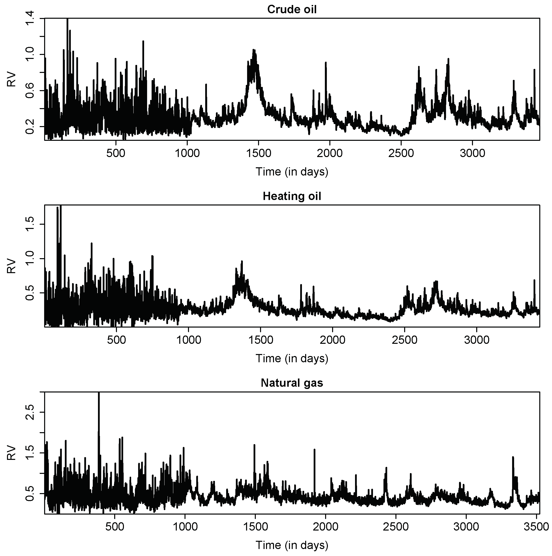
HAR-RV vs. All	0.1390	0.0013	0.0000

test results for the square root of RV. Such a robustness check is in order given that Figure 1 witnesses that the realized volatilities exhibited occasional large peaks during our sample period. The main finding of this robustness check is that we observe significant test results predominantly when we study the monthly forecast horizon, even though there are a few significant test results also for the weekly forecast horizon. Hence, the main finding of this robustness test is consistent with the finding from the baseline test results that we lay out in Table 2.

Eyeballing Figure 1 further reveals that the dynamics of the realized volatilities changed at roughly observation 1500. In order to account for this observations, we report in

Table 4. Test results for a shorter sample period. Results (p-values; robust heteroskedasticity and autocorrelation consistent standard errors) of the Clark–West tests for an equal mean-squared prediction error are based on robust standard errors. The classic HAR-RV model is the benchmark model, and the model extended to include climate-risk factors is the rival model. The alternative hypothesis is that the rival model has a smaller MSPE than the benchmark model. The parameter h denotes the forecast horizon (in days). The models are estimated using a rolling-estimation window of length 250 observations. The first 1500 forecasts are excluded.

Energy Source/Model	h = 1	h = 5	h = 22
Crude oil
HAR-RV vs. U.S. climate policy	0.4179	0.8580	0.6417
HAR-RV vs. International summits	0.5672	0.6027	0.0375
HAR-RV vs. Global warming	0.7781	0.9279	0.2166
HAR-RV vs. Natural disasters	0.4918	0.1456	0.0069
HAR-RV vs. Narrative factor	0.8732	0.4018	0.0419
HAR-RV vs. All	0.5897	0.3955	0.0041
Heating oil
HAR-RV vs. U.S. climate policy	0.5304	0.9520	0.5703
HAR-RV vs. International summits	0.3319	0.4189	0.1978
HAR-RV vs. Global warming	0.9795	0.2689	0.0344
HAR-RV vs. Natural disasters	0.3399	0.1456	0.0039
HAR-RV vs. Narrative factor	0.6495	0.0626	0.0029
HAR-RV vs. All	0.6820	0.1938	0.0013
Natural gas
HAR-RV vs. U.S. climate policy	0.0335	0.0567	0.0672
HAR-RV vs. International summits	0.6202	0.1076	0.0294
HAR-RV vs. Global warming	0.0593	0.0155	0.2473
HAR-RV vs. Natural disasters	0.3957	0.7876	0.9230
HAR-RV vs. Narrative factor	0.6737	0.3192	0.3637
HAR-RV vs. All	0.0875	0.0774	0.0439

results for a shorter sample period, that is, we delete the first 1500 forecasts before setting up the Clark–West test. The results are broadly in line with our baseline test results. We observe strong evidence of predictive value of the climate-risk factors at the monthly forecast horizon for crude oil and heating oil and, to a somewhat lesser extent, for natural gas. For natural gas, we further observe that half of the test results at the weekly forecast horizon are significant. We also observe, corroborating the results of our baseline forecasting experiment that we summarize in Table 2, that the test results for the full model that features all five climate-risk factors are significant at the monthly forecast horizon.

In

Table 5. Shrinkage results. Results (p-values; robust heteroskedasticity and autocorrelation consistent standard errors) of the Clark–West tests for an equal mean-squared prediction error are based on robust standard errors. The classic HAR-RV model is the benchmark model, and the model extended to include all climate-risk factors and estimated by the Lasso, Ridge, and elastic-net estimator is the rival model. The alternative hypothesis is that the rival model has a smaller MSPE than the benchmark model. The parameter h denotes the forecast horizon (in days). The models are estimated using a rolling-estimation window of length 250 observations.

Panel A: Results for $\mathit{RV}$
Energy Source/Models	h = 1	h = 5	h = 22
Crude oil
HAR-RV vs. Lasso	0.0267	0.0187	0.0000
HAR-RV vs. Ridge	0.0241	0.0098	0.0000
HAR-RV vs. Elastic net	0.1101	0.0175	0.0000
Heating oil
HAR-RV vs. Lasso	0.2876	0.2832	0.0000
HAR-RV vs. Ridge	0.0695	0.0759	0.0000
HAR-RV vs. Elastic net	0.1286	0.2807	0.0000
Natural gas
HAR-RV vs. Lasso	0.0972	0.1982	0.0761
HAR-RV vs. Ridge	0.0490	0.0231	0.1187
HAR-RV vs. Elastic net	0.1856	0.1332	0.0830
Panel B: Results for $\sqrt{\mathit{RV}}$
Energy Source/Models	h= 1	h= 5	h= 22
Crude oil
HAR-RV vs. Lasso	0.1660	0.1828	0.0001
HAR-RV vs. Ridge	0.0567	0.0271	0.0000
HAR-RV vs. Elastic net	0.2149	0.0986	0.0000
Heating oil
HAR-RV vs. Lasso	0.2901	0.5648	0.0000
HAR-RV vs. Ridge	0.1368	0.0638	0.0000
HAR-RV vs. Elastic net	0.2370	0.3025	0.0000
Natural gas
HAR-RV vs. Lasso	0.1745	0.0610	0.0708
HAR-RV vs. Ridge	0.1303	0.0142	0.0815
HAR-RV vs. Elastic net	0.2259	0.0453	0.1316

, we report test results that we obtain when we use three popular shrinkage estimators to estimate the HAR-RV cum all climate-risk factors model. The three shrinkage estimators are interesting for the purpose of our forecasting experiments because they identify a parsimonious forecasting model in a completely data-driven way. We consider the following three shrinkage estimators: the Lasso estimator, the Ridge-regression estimator, and an elastic net. The latter can be interpreted as a combination of the Lasso and Ridge-regression estimators. The test results show again that the climate-risk factors help to improve the accuracy of forecasts of the realized volatilities at the monthly forecast horizon relative to the accuracy of forecasts that we obtain from the benchmark HAR-RV model (estimated by ordinary-least squares). For crude oil and heating oil, all test results are significant ($h=22$), while the evidence of an improvement in forecast accuracy is weaker for natural gas. Moreover, the Ridge-regression estimator in particular tends to yield significant test results at the short and intermediate forecast horizons ($h=1,5$) even for the daily and weekly forecast horizon.

Table 6. Results for longer rolling-estimation windows. Results (p-values; robust heteroskedasticity and autocorrelation consistent standard errors) of the Clark–West tests for an equal mean-squared prediction error are based on robust standard errors. The classic HAR-RV model is the benchmark model, and the model extended to include all climate-risk factors and estimated by the Lasso, Ridge, and elastic-net estimator is the rival model. The alternative hypothesis is that the rival model has a smaller MSPE than the benchmark model. The parameter h denotes the forecast horizon (in days).

Energy Source/Model	Window	h = 1	h = 5	h = 22
Crude oil
HAR-RV vs. U.S. climate policy	500	0.8125	0.2109	0.1914
HAR-RV vs. International summits	500	0.5454	0.0930	0.0318
HAR-RV vs. Global warming	500	0.7039	0.0549	0.0021
HAR-RV vs. Natural disasters	500	0.3065	0.5165	0.0554
HAR-RV vs. Narrative factor	500	0.2015	0.2491	0.2085
HAR-RV vs. All	500	0.4081	0.0722	0.0002
HAR-RV vs. U.S. climate policy	1000	0.4376	0.7463	0.6232
HAR-RV vs. International summits	1000	0.0773	0.0181	0.0007
HAR-RV vs. Global warming	1000	0.7181	0.6931	0.4861
HAR-RV vs. Natural disasters	1000	0.8546	0.1863	0.1417
HAR-RV vs. Narrative factor	1000	0.7928	0.3893	0.9182
HAR-RV vs. All	1000	0.6716	0.1587	0.0290
Heating oil
HAR-RV vs. U.S. climate policy	500	0.1970	0.1188	0.0021
HAR-RV vs. International summits	500	0.7393	0.3008	0.0001
HAR-RV vs. Global warming	500	0.9930	0.9824	0.0001
HAR-RV vs. Natural disasters	500	0.3774	0.3479	0.0001
HAR-RV vs. Narrative factor	500	0.0334	0.1651	0.1616
HAR-RV vs. All	500	0.5975	0.4760	0.0000
HAR-RV vs. U.S. climate policy	1000	0.1026	0.0171	0.0351
HAR-RV vs. International summits	1000	0.0152	0.0019	0.0189
HAR-RV vs. Global warming	1000	0.0403	0.0080	0.0204
HAR-RV vs. Natural disasters	1000	0.8252	0.1242	0.0923
HAR-RV vs. Narrative factor	1000	0.5719	0.0712	0.2767
HAR-RV vs. All	1000	0.0961	0.0006	0.0059
Natural gas
HAR-RV vs. U.S. climate policy	500	0.1416	0.1903	0.1404
HAR-RV vs. International summits	500	0.2097	0.0478	0.0001
HAR-RV vs. Global warming	500	0.7952	0.5049	0.0000
HAR-RV vs. Natural disasters	500	0.4839	0.0500	0.0061
HAR-RV vs. Narrative factor	500	0.4007	0.4357	0.4119
HAR-RV vs. All	500	0.2878	0.0185	0.0000
HAR-RV vs. U.S. climate policy	1000	0.1256	0.0154	0.1264
HAR-RV vs. International summits	1000	0.0934	0.0407	0.0005
HAR-RV vs. Global warming	1000	0.6997	0.5893	0.1352
HAR-RV vs. Natural disasters	1000	0.7563	0.5389	0.7422
HAR-RV vs. Narrative factor	1000	0.6663	0.8124	0.3467
HAR-RV vs. All	1000	0.4207	0.0649	0.0032

reports the results we obtain when we use somewhat longer rolling-estimation windows (500 and 1000 observations) to estimate our forecasting models. The message to take home from the results summarized in Table 6 is that, on balance, there is evidence (somewhat stronger for the window that uses 500 than for the window that uses 1000 observations) that considering climate-risk factors as predictors of realized volatilities at a monthly forecast horizon yields forecasts that are superior relative to the forecasts computed by means of a benchmark HAR-RV model. For the monthly forecast horizon, we observe that the test results for the forecasting model that features all five climate-risk factors in its array of predictors are significant for both rolling-estimation windows.

As a further variant of our forecasting experiment, we report in

Table 7. Test results for a recursive-estimation window. Results (p-values; robust heteroskedasticity and autocorrelation consistent standard errors) of the Clark–West tests for an equal mean-squared prediction error are based on robust standard errors. The classic HAR-RV model is the benchmark model, and the model extended to include climate-risk factors is the rival model. The alternative hypothesis is that the rival model has a smaller MSPE than the benchmark model. The parameter h denotes the forecast horizon (in days). The models are estimated using a recursive-estimation window, where we use 250 observations as a training period to initialize the estimations.

Energy Source/Model	h = 1	h = 5	h = 22
Crude oil
HAR-RV vs. U.S. climate policy	0.3419	0.1665	0.2965
HAR-RV vs. International summits	0.5830	0.1402	0.0417
HAR-RV vs. Global warming	0.2578	0.5709	0.0725
HAR-RV vs. Natural disasters	0.1645	0.5830	0.0912
HAR-RV vs. Narrative factor	0.4531	0.2506	0.5766
HAR-RV vs. All	0.1050	0.1240	0.0426
Heating oil
HAR-RV vs. U.S. climate policy	0.2662	0.1837	0.1200
HAR-RV vs. International summits	0.7032	0.0952	0.0250
HAR-RV vs. Global warming	0.3849	0.2267	0.0162
HAR-RV vs. Natural disasters	0.2209	0.5308	0.1594
HAR-RV vs. Narrative factor	0.2220	0.1542	0.2041
HAR-RV vs. All	0.1114	0.0976	0.0215
Natural gas
HAR-RV vs. U.S. climate policy	0.2632	0.2250	0.2309
HAR-RV vs. International summits	0.5317	0.3901	0.0693
HAR-RV vs. Global warming	0.6952	0.2123	0.1622
HAR-RV vs. Natural disasters	0.6785	0.0174	0.0012
HAR-RV vs. Narrative factor	0.2777	0.1704	0.0220
HAR-RV vs. All	0.5941	0.0132	0.0003

results that we obtain when we study a recursive-estimation window. The changing dynamics of the realized volatilities documented in Figure 1 imply that a recursive-estimation window is not our preferred choice for the analysis of our data. Notwithstanding, it is interesting briefly to sketch the results for a recursive-estimation window. As in the case of a rolling-estimation window, we observe several significant test results for the monthly forecast horizon. The forecast model that uses all five climate-risk factors as predictors yields always significant test results at the long forecast horizon.

Based on the suggestion of an anonymous referee to better understand the possible statistical reasons behind the weak in-sample evidence relative to the stronger out-of-sample performance of the climate risks variables, we conducted the multiple structural break tests of [50] on the augmented HAR-RV model that involves all the five predictors of climate risks. We found five breaks (specific dates of which are available upon request from the authors) each at h = 1, 5 and 22 for all three of the energy prices. Given the evidence of structural breaks, it is not surprising that the full-sample regressions provide only weak evidence that the climate-risk factors matter for in-sample predictability.

In this regard, it is also worth mentioning that plots (complete details of which are available upon request from the authors) of the time-varying coefficients of the climate-risk factors estimated by means of a rolling-estimation window indicate that the signs of the estimated coefficients changed over time, possibly reflecting that the relative importance of the multiple opposing channels through which climate risks affect the realized volatility was not constant over time. The full-sample regressions capture the “average sign” of the coefficients and, thereby, recover only a weak predictive value of the climate-risk factors for realized volatility. An out-of-sample analysis, in contrast, is better suited to recover such changing patterns in the link between realized volatility and the climate-risk factors, as it is based on time-varying parameter estimates of the models derived from rolling and recursive windows. Intuition, thus, suggests that an out-of-sample analysis can be expected to yield stronger evidence of predictability than a full-sample analysis, which, in turn, is vindicated by our out-of-sample forecasting results.

Finally, we consider the possibility that policymakers and forecasters are interested in forecasts for horizons that extend beyond one month. Moreover, one can conceive situations in which policymakers and forecasters differentiate between positive and negative forecast errors. An underestimation of energy-price volatility in the wake of an energy crisis that gathers steam, for example, might be costlier for a policymaker in terms of approval rates than a corresponding overestimation of the same absolute seize. Overestimation of energy-price volatility, in turn, may result in excessive storage and high opportunity costs. In order to model a potential differential weighting of under- and over-estimations of realized volatility, we use the loss function studied by [51,52]. The loss function is given by $L=(\alpha +(1-2\alpha )I_{fe<0}){\left|fe\right|}^p$, where $fe$ denotes the forecast error and $I_{fe<0}$ denotes the indicator function. Setting $p=1$ results in a quasi-linear function that depends on the absolute forecast error (L1 loss), while setting $p=2$ restricts the loss function to be of the quadratic type (L2 loss). The (as-)symmetry parameter, $\alpha \in (0,1)$ governs the relative loss from an under-or overestimation of realized volatility. For $\alpha =0.5$, we obtain a symmetric loss function. For $\alpha \ne 0.5$, we obtain $\alpha >0.5$ ($\alpha <0.5$), the loss from under-estimating (over-estimating) realized volatility exceeds the loss from an overestimation (underestimation) of the same (absolute) size.

Figure 4 summarizes the results for this loss function. We report results for forecast horizons from one day to three months (that is, 66 days). The figure displays the loss ratio that we obtain by dividing the sum of the loss from the out-of-sample forecast errors as computed by means of the HAR-RV benchmark model by the the sum of the loss from the out-of-sample forecast errors as computed by means of the HAR-RV model extended to include all climate-risk factors. A ratio exceeding unity, thus, indicates that the extended model has a better out-of-sample forecasting performance than the benchmark model, given the (as-)symmetry parameter, $\alpha$. The results show that the forecasting gains from using the climate-risk factors as predictors tend to increase in the forecast horizon for the case of a symmetric loss function. In the asymmetric case, in turn, the forecasting gains for long forecast horizons are mainly concentrated in the region where $\alpha >0.5$ when we study crude oil and a L2 loss function. For a L2 loss function, the forecasting gains are more evenly distributed across the interval of the asymmetry parameter. For heating oil and natural gas, in turn, the forecasting gains in the case of long forecast horizons are strongest in the region where $\alpha <0.5$.

3.2. Implications for Economic Agents

At this stage, it is important to highlight the implications of our findings for various groups of economic agents. From the perspective of a policymaker, given that energy-price volatility is associated with movements in global economic growth [18,19], the high-frequency forecasts of the path of variability of the energy market emanating from climate risks can be fed into MIDAS models to obtain nowcasts of low-frequency economic activity-related variables [40]. This, in turn, will allow policy authorities to design appropriate decisions well-ahead of time before data on low-frequency variables become available, and prevent possible recessions in the wake of heightened energy-market volatility resulting from climate risks. Moreover, because investments in energy markets are now considered as alternative opportunities to traditional financial assets due to the financialization of the energy sector [12,13,14], having available accurate forecasts of the future path of the realized volatility of energy-price returns is of paramount importance for market participants, who need volatility forecasts as key inputs to their investment decisions and portfolio choices [20]. In this regard, it is also important to note that daily volatility forecasts feature prominently in the context of VaR estimates [39].

Additionally, given that our empirical findings indicate that climate risks can forecast energy-market volatility, particularly in the longer-run, models need to be developed by academics to theoretically conceptualize such a relationship. In other words, one would need to go beyond the existing models depicting the impact of climate risks on the first-moment of energy-price returns. While doing this, given relatively weak in-sample, but stronger out-of-sample, forecasting results, theoretical energy economists would need to keep in mind the fact that the structural parameters of the models should in fact be evolving over time, and not constant, along the lines of time-varying Dynamic Stochastic General Equilibrium Models (see for example, [53,54,55]).

4. Concluding Remarks

The current European energy-price crisis is a reminder that the prices of crude and heating oil as well as of natural gas play a prominent role not only in discussions of the economic consequences of large swings in energy prices, but also in debates in policy circles of key issues related to energy security. Our empirical research aims to inform such debates by analyzing the role of climate-risk factors for forecasting future realizations of the realized volatilities of the returns of the prices of three key energy sources: crude oil, heating oil, and natural gas. The importance of climate-risk factors for energy security most likely will increase in the future and for this reason, it is of utmost importance for policymakers to better understand whether climate-risk factors contain useful information for large swings in energy prices.

The empirical findings that we have reported in this research can help to develop a better understanding of the link between climate risks and volatile energy prices. We have documented strong evidence that the five climate-risk factors that we have considered in our out-of-sample forecasting experiments tend to add to the accuracy of out-of-sample forecasts of the realized volatilities of the returns of the prices of crude oil, heating oil, and natural gas at a monthly and, in some cases, also at a shorter forecast horizon. Moreover, we have also studied longer forecast horizons of up to three months, where we have taken into account that policymakers and forecasters encounter a loss from an underestimation of realized volatility that differs from the cost of an overestimation of the same absolute size.

As an avenue for future research, it is interesting to shed light on how climate-risk factors contribute to the performance of out-of-sample forecasting of energy-price movements relative to other sources of risk like, for example, geopolitical risks. This is important, given the evidence that geopolitical risks have tended to drive the movements in energy prices historically (see, for example, [56]). It is also interesting to study whether the evidence we have reported in this research extends to markets for other natural resources. In this regard, the link between climate-risk factors and the volatility of movements of prices of important agricultural commodities is particularly important, as might also be the case of precious metals which have been considered as traditional safe-havens in the wake of global risks and uncertainties [57]. We hope that our research will set the stage for such future empirical analyses. Moreover, while there exist theoretical models relating energy prices to climate risks, in the future, a theory should be developed to explain not only variance, but the overall energy market volatility directly due to the effects of climate-related uncertainties.

References

1. Barnett, M.D. A Run on Oil: Climate Policy, Stranded Assets, and Asset Prices. Ph.D. Thesis, The University Chicago, Chicago, IL, USA, 2019. Available online: https://knowledge.uchicago.edu/record/1908?ln=en (accessed on 1 October 2021).
2. Dike, J.C. Does climate change mitigation activity affect crude oil prices? Evidence from dynamic panel model. J. Energy 2014, 2014, 514029. [Google Scholar] [CrossRef] [Green Version]
3. Asai, M.; Gupta, R.; McAleer, M. The impact of jumps and leverage in forecasting the co-volatility of oil and gold futures. Energies 2019, 12, 3379. [Google Scholar] [CrossRef] [Green Version]
4. Asai, M.; Gupta, R.; McAleer, M. Forecasting volatility and co-volatility of crude oil and gold futures: Effects of leverage, jumps, spillovers, and geopolitical risks. Int. J. Forecast. 2020, 36, 933–948. [Google Scholar] [CrossRef] [Green Version]
5. Degiannakis, S.; Filis, G.; Panagiotakopoulou, S. Oil price shocks and uncertainty: How stable is their relationship over time? Econ. Model. 2018, 72, 42–53. [Google Scholar] [CrossRef] [Green Version]
6. Shahzad, S.J.H.; Gupta, R.; Demirer, R.; Pierdzioch, C. Oil shocks and directional predictability of macroeconomic uncertainties of developed economies: Evidence from high-frequency data. Scott. J. Political Econ. 2021. Available online: https://onlinelibrary.wiley.com/doi/abs/10.1111/sjpe.12280 (accessed on 1 October 2021). [CrossRef]
7. Bakas, D.; Triantafyllou, A. The impact of uncertainty shocks on the volatility of commodity prices. J. Int. Money Financ. 2018, 87, 96–111. [Google Scholar] [CrossRef] [Green Version]
8. Bakas, D.; Triantafyllou, A. Commodity price volatility and the economic uncertainty of pandemics. Econ. Lett. 2020, 193, 109283. [Google Scholar] [CrossRef]
9. Battiston, S.; Dafermos, Y.; Monasterolo, I. Climate risks and financial stability. J. Financ. Stab. 2021, 54, 100867. [Google Scholar] [CrossRef]
10. Giglio, S.; Kelly, B.; Stroebel, J. Climate finance. Annu. Rev. Financ. Econ. 2021, 33, 1011–1023. [Google Scholar] [CrossRef]
11. Flori, A.; Pammolli, F.; Spelta, A. Commodity prices co-movements and financial stability: A multidimensional visibility nexus with climate conditions. J. Financ. Stab. 2021, 54, 100876. [Google Scholar] [CrossRef]
12. Bampinas, G.; Panagiotidis, T. On the relationship between oil and gold before and after Financial Crisis: Linear, nonlinear and time-varying causality testing. Stud. Nonlinear Dyn. Econom. 2015, 19, 657–668. [Google Scholar] [CrossRef]
13. Bampinas, G.; Panagiotidis, T. Oil and stock markets before and after financial crises: A local Gaussian correlation approach. J. Futur. Mark. 2017, 37, 1179–1204. [Google Scholar] [CrossRef]
14. Bonato, M. Realized correlations, betas and volatility spillover in the agricultural commodity market: What has changed? J. Int. Financ. Mark. Inst. Money 2019, 62, 184–202. [Google Scholar] [CrossRef]
15. Nazlioglu, S.; Soytas, U.; Gupta, R. Oil prices and financial stress: A volatility spillover analysis. Energy Policy 2015, 82, 278–288. [Google Scholar] [CrossRef] [Green Version]
16. Gupta, R.; Kanda, P.T.; Wohar, M.E.; Tiwari, A.K. Time-varying predictability of oil market movements over a century of data: The role of US financial stress. N. Am. J. Econ. Financ. 2019, 50, 100994. [Google Scholar] [CrossRef]
17. Gkillas, K.; Gupta, R.; Pierdzioch, C. Forecasting realized oil-price volatility: The role of financial stress and asymmetric loss. J. Int. Money Financ. 2020, 104, 102137. [Google Scholar] [CrossRef]
18. van Eyden, R.; Difeto, M.; Gupta, R.; Wohar, M.E. Oil price volatility and economic growth: Evidence from advanced economies using more than a century of data. Appl. Energy 2019, 233, 612–621. [Google Scholar] [CrossRef] [Green Version]
19. Salisu, A.A.; Gupta, R.; Olaniran, A. The effect of oil uncertainty shock on real GDP of 33 countries: A global VAR approach. Appl. Econ. Lett. 2021. [Google Scholar] [CrossRef]
20. Poon, S.-H.; Granger, C.W.J. Forecasting volatility in financial markets: A review. J. Econ. Lit. 2003, 41, 478–539. [Google Scholar] [CrossRef]
21. McAleer, M.; Medeiros, M.C. Realized volatility: A review. Econom. Rev. 2008, 27, 10–45. [Google Scholar] [CrossRef]
22. Corsi, F. A simple approximate long-memory model of realized volatility. J. Financ. Econom. 2009, 7, 174–196. [Google Scholar] [CrossRef]
23. Chan, J.C.C.; Grant, A. Modeling energy price dynamics: GARCH versus stochastic volatility. Energy Econ. 2016, 54, 182–189. [Google Scholar] [CrossRef] [Green Version]
24. Lux, T.; Segnon, M.; Gupta, R. Forecasting crude oil price volatility and value-at-risk: Evidence from historical and recent data. Energy Econ. 2016, 56, 117–133. [Google Scholar] [CrossRef] [Green Version]
25. Faccini, R.; Matin, R.; Skiadopoulos, G. Dissecting Climate Risks: Are They Reflected in Stock Prices? Available online: https://ssrn.com/abstract=3795964 (accessed on 1 October 2021).
26. Degiannakis, S.; Filis, G. Forecasting oil price realized volatility using information channels from other asset classes. J. Int. Money Financ. 2017, 76, 28–49. [Google Scholar] [CrossRef] [Green Version]
27. Bonato, M.; Gkillas, K.; Gupta, R.; Pierdzioch, C. Investor happiness and predictability of the realized volatility of oil price. Sustainability 2020, 12, 4309. [Google Scholar] [CrossRef]
28. Bouri, E.; Gkillas, K.; Gupta, R.; Pierdzioch, C. Infectious diseases, market uncertainty and realized volatility of oil. Energies 2020, 13, 4090. [Google Scholar] [CrossRef]
29. Demirer, R.; Gupta, R.; Pierdzioch, C.; Shahzad, S.J.H. The predictive power of oil price shocks on realized volatility of oil: A note. Resour. Policy 2020, 69, 101856. [Google Scholar] [CrossRef]
30. Demirer, R.; Gkillas, K.; Gupta, R.; Pierdzioch, C. Risk aversion and the predictability of crude oil market volatility: A forecasting experiment with random forests. J. Oper. Res. Soc. 2021. [Google Scholar] [CrossRef]
31. Gupta, R.; Pierdzioch, C. Forecasting the volatility of crude oil: The role of uncertainty and spillovers. Energies 2021, 14, 4173. [Google Scholar] [CrossRef]
32. Luo, J.; Demirer, R.; Gupta, R.; Ji, Q. Forecasting oil and gold volatilities with sentiment indicators under structural breaks. Energy Econ. 2021. Available online: https://www.up.ac.za/media/shared/61/WP/wp_2021_30.zp202081.pdf (accessed on 1 October 2021).
33. Salisu, A.A.; Gupta, R.; Bouri, E.; Ji, Q. Mixed-frequency forecasting of crude oil volatility based on the information content of global economic conditions. J. Forecast. 2021. [Google Scholar] [CrossRef]
34. Lyócsa, Š.; Molnárc, P. Exploiting dependence: Day-ahead volatility forecasting for crude oil and natural gas exchange-traded funds. Energy 2018, 155, 462–473. [Google Scholar] [CrossRef]
35. Fałdziński, M.; Fiszeder, P.; Orzeszko, W. Forecasting volatility of energy commodities: Comparison of GARCH Models with Support Vector Regression. Energies 2021, 14, 6. [Google Scholar] [CrossRef]
36. Balcilar, M.; Bouri, E.; Gupta, R.; Pierdzioch, C. El Niño, La Nña, and the forecastability of the realized variance of heating oil price movements. Sustainability 2021, 13, 7987. [Google Scholar] [CrossRef]
37. Bouri, E.; Gupta, R.; Pierdzioch, C.; Salisu, A.A. El Niño and forecastability of oil-price realized volatility. Theor. Appl. Climatol. 2021, 144, 1173–1180. [Google Scholar] [CrossRef]
38. Demirer, R.; Gupta, R.; Nel, J.; Pierdzioch, C. Effect of Rare Disaster Risks on Crude Oil: Evidence from El Niño from Over 145 Years of Data. Theor. Appl. Climatol. 2021. [Google Scholar] [CrossRef]
39. Ghysels, E.; Valkanov, R. Forecasting volatility with MIDAS. In Handbook of Volatility Models and Their Applications; Bauwens, L., Hafner, C., Laurent, S., Eds.; John Wiley & Sons, Inc.: Hoboken, NJ, USA, 2012; pp. 383–401. [Google Scholar]
40. Bańbura, M.; Giannone, D.; Reichlin, L. Nowcasting. In Oxford Handbook on Economic Forecasting; Clements, M., Hendry, D., Eds.; Oxford University Press: Oxford, UK, 2011; pp. 63–90. [Google Scholar]
41. Xiu, D. Quasi-maximum likelihood estimation of volatility with high frequency data. J. Econom. 2010, 159, 235–250. [Google Scholar] [CrossRef]
42. Blei, D.M.; Ng, A.Y.; Jordan, M.I. Latent Dirichlet Allocation. J. Mach. Learn. Res. 2003, 3, 993–1022. [Google Scholar]
43. Müller, U.A.; Dacorogna, M.M.; Davé, R.D.; Olsen, R.B.; Pictet, O.V. Volatilities of different time resolutions—Analyzing the dynamics of market components. J. Empir. Financ. 1997, 4, 213–239. [Google Scholar] [CrossRef]
44. Charfeddine, L. True or spurious long memory in volatility: Further evidence on the energy futures markets. Energy Policy 2014, 71, 76–93. [Google Scholar] [CrossRef]
45. Niu, H.; Wang, J. Return volatility duration analysis of NYMEX energy futures and spot. Energy 2017, 140, 837–849. [Google Scholar] [CrossRef]
46. R Core Team. R: A Language and Environment for Statistical Computing; R Foundation for Statistical Computing: Vienna, Austria, 2021; Available online: https://www.R-project.org/ (accessed on 1 October 2021).
47. Friedman, J.; Hastie, T.; Tibshirani, R. Regularization paths for Generalized Linear Models via coordinate descent. J. Stat. Softw. 2010, 33, 1–22. [Google Scholar] [CrossRef] [PubMed] [Green Version]
48. Campbell, J.Y. Viewpoint: Estimating the equity premium. Can. J. Econ. 2008, 41, 1–21. [Google Scholar] [CrossRef] [Green Version]
49. Clark, T.E.; West, K.D. Approximately normal tests for equal predictive accuracy in nested models. J. Econom. 2007, 138, 291–311. [Google Scholar] [CrossRef] [Green Version]
50. Bai, J.; Perron, P. Computation and analysis of multiple structural change models. J. Appl. Econom. 2003, 18, 1–22. [Google Scholar] [CrossRef] [Green Version]
51. Elliott, G.; Komunjer, I.; Timmermann, A. Estimation and testing of forecast rationality under flexible loss. Rev. Econ. Stud. 2005, 72, 1107–1125. [Google Scholar] [CrossRef]
52. Elliott, G.; Komunjer, I.; Timmermann, A. Biases in macroeconomic forecasts: Irrationality or asymmetric loss? J. Eur. Econ. Assoc. 2008, 6, 122–157. [Google Scholar] [CrossRef]
53. Galvão, A.B.; Giraitis, L.; Kapetanios, G.; Petrova, K. A time varying DSGE model with financial frictions. J. Empir. Financ. 2016, 38, 690–716. [Google Scholar] [CrossRef] [Green Version]
54. Kapetanios, G.; Masolo, R.M.; Petrova, K.; Waldron, M. A time-varying parameter structural model of the UK economy. J. Econ. Dyn. Control 2021, 106, 103705. [Google Scholar] [CrossRef]
55. Petrova, K. Quasi-bayesian estimation of time-varying volatility in DSGE models. J. Time Ser. Anal. 2019, 40, 151–157. [Google Scholar] [CrossRef]
56. Demirer, R.; Gupta, R.; Suleman, M.T.; Wohar, M.E. Time-varying rare disaster risks, oil returns and volatility. Energy Econ. 2018, 75, 239–248. [Google Scholar] [CrossRef] [Green Version]
57. Boubaker, H.; Cunado, J.; Gil-Alana, L.A.; Gupta, R. Global crises and gold as a safe haven: Evidence from over seven and a half centuries of data. Phys. A Stat. Mech. Its Appl. 2020, 540, 123093. [Google Scholar] [CrossRef] [Green Version]
Figure 1. Realized volatilities. RV denotes the realized variance of the returns of the prices of the respective metals. The sample period is 3 January 2001–27 November 2019.
Energies 14 08085 g001
Figure 2. Autocorrelation functions. ACF denotes the autocorrelation function of the realized volatility of the returns of the prices of the respective metals. The dashed horizontal line denotes the 95% confidence line. The sample period is 3 January 2001–27 November 2019.
Energies 14 08085 g002
Figure 3. Climate risks. The sample period is 3 January 2001–27 November 2019.
Energies 14 08085 g003
Figure 4. Loss ratios for longer forecast horizons. The parameter α captures the (as-)symmetry of the loss function. The loss function is of the L = ( α + ( 1 2 α ) I f e < 0 ) | f e | p , where f e denotes the forecast error and the parameter p governs whether the loss function is of the L1 (quasi-linear function that depends on the absolute forecast error) or L2 (quadratic loss) type. The nominator of the loss ratio is given by the sum of the loss from the out-of-sample forecast errors as computed by means of the HAR-RV benchmark model. The denominator of the loss ratio is given by the sum of the loss from the out-of-sample forecast errors as computed by means of the HAR-RV model extended to include all climate-risk factors. A ratio exceeding unity indicates that the extended model has a better out-of-sample forecasting performance than the benchmark model, given the (as-)symmetry parameter, α . It should be noted that the representation of the numerical values of the loss ratio by colors is not identical across the three panels of this figure.
Energies 14 08085 g004