Torque Vectoring Control of RWID Electric Vehicle for Reducing Driving-Wheel Slippage Energy Dissipation in Cornering

Abstract

The anxiety of driving range and inconvenience of battery recharging has placed high requirements on the energy efficiency of electric vehicles. To reduce driving-wheel slip energy consumption while cornering, a torque vectoring control strategy for a rear-wheel independent-drive (RWID) electric vehicle is proposed. First, the longitudinal linear stiffness of each driving wheel is estimated by using the approach of recursive least squares. Then, an initial differential torque is calculated for reducing their overall tire slippage energy dissipation. However, before the differential torque is applied to the two side of driving wheels, an acceleration slip regulation (ASR) is introduced into the overall control strategy to avoid entering into the tire adhesion saturation region resulting in excessive slip. Finally, the simulations of typical manoeuvring conditions are performed to verify the veracity of the estimated tire longitudinal linear stiffness and effectiveness of the torque vectoring control strategy. As a result, the proposed torque vectoring control leads to the largest reduction of around 17% slip power consumption for the situations carried out above.

1. Introduction

Electric vehicles are receiving growing attention because of the advantages of high integration, fast motor response, and their light weight due to a compact driveline, as well as less pollution and their energy-saving potential. However, compared with traditional vehicles, electric vehicles still have the drawback of shorter mileage, insufficient public charging facilities, and time-consuming charging. Hence, the technological progress of electric vehicles still needs to be noticed and promoted [1]. As one of the essential aspects, to improve the mileage of electric vehicles not only do large-capacity batteries have to be developed to break through current battery technology, but also an energy-saving control strategy should be adopted [2].

At present, some scholars have conducted research in the energy-saving control strategy of electric vehicles in two aspects. Most scholars focus on motor energy consumption. Considering the copper loss and iron loss of the non-motor rotating with the non-driving wheel, J. GU established the comprehensive energy efficiency model of the permanent magnet synchronous motor including the inverter to study the energy efficiency optimization of a four-wheel independently actuated electric vehicle [3]. Zhang H aimed at neutral steering, attempting to distribute the torque of every driving wheel in order to reduce the cornering resistance as far as possible [4]. Koehler S proposed real-time optimization of the vehicle’s driving torque to achieve the highest driving efficiency [5]. Pennycott A took the motor efficiency into account, and studied the torque vectoring ratio of each driving wheel to minimize the energy consumption of the vehicle [6]. Pierpaolo P proposed an optimized controller for energy management, based on dynamic programming (DP) and receding horizon (RH) approaches to reduce the energy consumption [7]. Furthermore, several scholars have concentrated on the tire energy consumption. Kobayashi T considered tire stiffness as a function that is proportional to its normal load and used the tire stiffness in the tire slip consumption function to obtain the optimal yaw moment [8]. Himeno H calculated the tire consumption using the theoretical tire force value obtained from the brush model with the two inputs of tire slip ratio and slip angle [9]. Sun W proposed the genetic algorithm-particle swarm optimization hybrid algorithm (GA-PSO) to optimize the torque distribution coefficient offline [10]. Suzuki Y and Wang Y calculated the slip ratio by real-time tire stiffness and the tire driving force observed [11,12], and then established a function of the sum of the slip ratio square of all driving wheels to distribute the torque [13]. Wang J proposed a driving energy management strategy for four-wheel independent-drive electric vehicle (4WIDEV) based on multi-objective online optimization of four-wheel torque distribution [14]. Lin C proposed a vehicle drive control strategy developed to allow optimal wheel torque distribution under combined conditions while accelerating and cornering [15].

In summary, most of the precious studies focus on the energy consumption considering the effect of the motor efficiency, and there are several studies attaching great importance to tire stiffness for minimizing the tire slip energy consumption. However, tire stiffness is not only related to the normal load, but also related to the tire–road friction coefficient and other parameters [16,17], so it is not accurate enough to set the tire stiffness proportional to the normal load. Moreover, minimum slip ratio does not mean minimum slip energy consumption and using the sum of slip ratio square to distribute the torque is not suitable. Therefore, an appropriate function based on the real-time tire linear longitudinal stiffness to minimize tire slip energy should be built to achieve energy saving.

Based on the analysis above, this paper proposes the torque vectoring control of a rear-wheel independent-drive electric vehicle while cornering to decrease the slip ratio and minimize the tire slip energy consumption with the precondition of stable and safe driving. Firstly, the tire energy consumption including tire slip ratio and tire longitudinal slip consumption will be analyzed theoretically to dig out the absolute mechanism of torque vectoring. Secondly, tire linear longitudinal stiffness (TLLS) is introduced and first defined for a better torque vectoring control, for which an estimator is then designed to acquire an accurate and real-time value. Thirdly, the vehicle model and the whole torque vectoring strategy are established. Finally, simulations for the proposed torque vectoring control are carried out to verify its validity.

2. Theoretical Analysis of the Effect of Torque Vectoring on Tire Slip

Torque vectoring (TV) control develops from active differential [18], which realizes a random torque transferring between the driving wheels. However, for an RWID electric vehicle, how torque vectoring control affects tire slip ratio and slip energy is of great importance to determine the differential torque between the driving wheels at each moment while turning. Therefore, the mechanism of torque vectoring has to be further studied.

Since the normal load transfer between driving wheels while the vehicle is turning, the tire longitudinal stiffness varies a lot. The driving force can be expressed in the linear area of the tire as follows [19]:

$$F_{xi}=k_i\cdot s_i$$

(1)

where, $F_{xi}$ is the longitudinal force, $k_i$ is the driving stiffness of the $i$-th wheel, $s_i$ is the slip ratio of the $i$-th wheel, $i=1~2$.

When the vehicle is turning, if the total required torque $T_{req}$ is distributed meanly to the two rear driving wheels as usual, the torque of each wheel is as follows:

$$T_w=T_n=\frac{T_{req}}{2}$$

(2)

where, $T_n$ and $T_w$ are the driving torque of inner wheel and outer wheel, respectively.

Figure 1 shows the tires’ longitudinal force characteristics with the slip ratios of inner and outer driving wheels. It can be easily found that the slip of the outer wheel is smaller than that of the inner wheel if equal tire longitudinal force is generated due to laterally transfer of normal force of the two side of wheels resulted from vehicle body roll movement while corning. Therefore, if equal driving torque is distributed between two side of wheels, the outer wheel cannot make full use of the adhesive condition though it still has adhesion margin, and the inner wheel may also easily slip due to comparative excessive traction force requirement.

When applying the torque vectoring control is, a differential torque $\Delta T$ is formed and torques of the two wheels are controlled as follow:

$$\begin{array}{l}{T}_w+T_n=T_{req}\\ T_w-T_n=\Delta T\end{array}$$

(3)

After torque vectoring, the slip ratios have changed a lot and they could be shown as follows:

$$s_{in}^{\prime }=s_{in}-\frac{\Delta T}{2r_w{k}_{in}}$$

(4)

$$s_{out}^{\prime }=s_{out}+\frac{\Delta T}{2r_w{k}_{out}}$$

(5)

where, $k_{in}$ and $k_{out}$ are the tire longitudinal stiffness of the inner and outer driving wheels, respectively; $s_{in}^{\prime }$ and $s_{out}^{\prime }$ are the tire slip ratio of the inner and outer driving wheels with torque vectoring control, respectively.

Therefore, the variation of the average slip ratio of the rear axle could be shown as follows:

$$\Delta s_{avg}=\frac{\Delta T}{4r_w}\left(\frac{1}{k_{out}}-\frac{1}{k_{in}}\right)$$

(6)

Since $k_{out}>k_{in}$, the variation of the outer tire slip ratio is less than that of the inner one, so $\Delta s_{avg}<0$ and that means the total tire wear of the rear axle descends.

As is known, due to the slip ratio, the driving efficiency has always been lower than 100% which means the longitudinal force works in the direction of tire slip velocity and extra tire slip energy consumption is caused finally.

For the whole vehicle, the total slip energy consumption can be expressed as follows:

$$P_{ws}={\displaystyle \sum F_{xi}\cdot V_{si}}={\displaystyle \sum F_{xi}\cdot V_i}\cdot s_i$$

(7)

where, $P_{ws}$ is the total slip energy consumption; $F_{xi}$, $V_{si}$ and $V_i$ are the longitudinal force, the longitudinal slip velocity and the rotation linear velocity for the $i$-th driving wheel.

Therefore, combining Equations (1), (4), (5), with (7), the total tire slip energy consumption in every moment, in other words, the slip power consumption $P_{ws}$ is defined as follows:

$$P_{ws}=V_{out}\frac{{\left(\frac{T_{req}}{2r_w}+\frac{\Delta T}{2r_w}\right)}^2}{k_{out}}+V_{in}\frac{{\left(\frac{T_{req}}{2r_w}-\frac{\Delta T}{2r_w}\right)}^2}{k_{in}}$$

(8)

where, $V_{out}$ and $V_{in}$ are the rotation linear velocity of the outer wheel and the inner wheel respectively.

From the equation above, it can be seen that slip energy consumption is related to the product of tire slip ratio and longitudinal force. Only an appropriate torque vectoring control is able to ensure the decrease of overall wear of the drive wheel as well as the loss of tire slip energy consumption in the condition of the invariable total required driving torque.

Apparently, the total tire slip energy consumption in every moment is a quadratic function about the tire longitudinal stiffness and the differential torque. As a result, the differential torque will never be a casual value, but a specific one according to the tires longitudinal stiffness for minimizing the total tire slip energy consumption.

To sum up, torque vectoring can reduce the rear axle average slip ratio with more differential torque, which can reduce the total tire wear of the driving axle. Apart from this, torque vectoring can also pull the slip energy consumption down, but only the specific differential torque can achieve the best energy saving effect. Considering all the factors above, torque vectoring control is determined for minimizing slip energy consumption based on the incessantly shifty tire longitudinal stiffness and identifying the longitudinal stiffness of the driving wheels is an important task that needs to be carried out next.

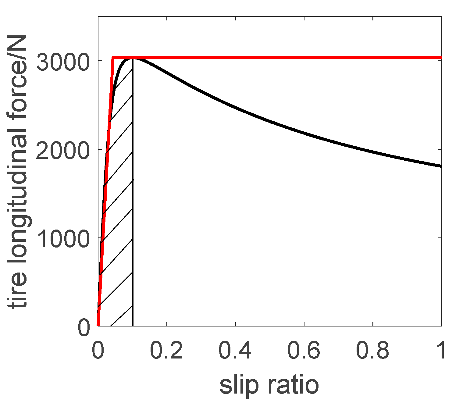
3. The Definition and Estimation for Tire Linear Longitudinal Stiffness (TLLS)

3.1. The Definition of TLLS

Because the linear tire model and the non-linear tire model are of great consistency when lateral acceleration is under 0.4 g [20], and the lateral acceleration is generally low when the vehicle runs normally, the theoretical tire model as shown in Figure 2 is simplified into an oblique line close to the theoretical curve passing the origin and a transverse line passing the peak of the original curve. In this way, the relationship between longitudinal force and tire slip ratio can easily and clearly be expressed.

Apparently, the slope of the simplified tire adhesion curve in the linear region is different from the tire longitudinal stiffness defined in ‘Tire and Vehicle Dynamics’ [21], so TLLS is defined to describe the characteristic. The value of TLLS is several orders smaller compared to tire longitudinal stiffness. Due to a moderate size, even if there are some awful deviations or terrible noises for getting the longitudinal force and slip ratio, the TLLS will be hardly ever affected. Therefore, the differential torque calculated can reflect the driving condition more accurately and the adhesion characteristic can play a full and active role in the turning process. Next, TLLS will be regarded as an essential factor to allocate the torque between the driving wheels.

3.2. Estimator for TLLS

The longitudinal simulation, a really tiny one when the vehicle is running stably, is generally only several percent of the slip ratio [22]. Therefore, TLLS could be estimated in the little slip ratio area. Since TLLS is a factor determined by tire characteristic, but influenced a lot by tire normal load as well as the coefficient of road adhesion, TLLS varies while cornering and the estimation is comparatively significant [23,24].

Figure 3 illustrates the single driving wheel model, and the dynamic differential equation is shown as follows:

$$I_w\frac{\mathrm{d}{\omega }_i}{\mathrm{d}t}=T_i-F_{xi}\cdot r_w$$

(9)

where, $I_w$ is the rotational inertia of the wheel; ${\omega }_i$ is the rotational speed.

According to the advantage of easy acquisition of the torque for electric vehicles, the longitudinal force could be observed by a driving force observer (DFO) [11,12] designed from the single driving wheel model. Therefore, the observed longitudinal force can be obtained.

The slip ratio for each wheel can be calculated as follows [19]:

$$s_i=\frac{\left|u_i-{\omega }_i\cdot r_w\right|}{\max \left(u_i,{\omega }_i\cdot r_w\right)}$$

(10)

where, $u_i$ is the center speed of the wheel.

In order to accurately estimate the tire linear longitudinal stiffness in the current state, it is necessary to select an appropriate adaptive filtering algorithm. Moreover, the cornering condition generally takes a short time, the estimation of the tire linear longitudinal stiffness not only requires high accuracy, but also has a faster convergence rate. By now, TLLS could be estimated by constructing a recursive least squares (RLS) [25,26] problem, and the standard format of the method is as follows:

$$y\left(t\right)={\phi }^T\left(t\right)\cdot \theta \left(t\right)$$

(11)

where, $y\left(t\right)$ is the output, $y\left(t\right)=\frac{T_i-I_w\frac{\mathrm{d}{\omega }_i}{\mathrm{d}t}}{r_w}$; $\phi \left(t\right)$ is the regression vector, $\phi \left(t\right)=s_i$; $\theta \left(t\right)$ is the estimation parameter, $\theta \left(t\right)=k_i$.

And the detailed steps are shown as follow:

1. Initialize TLLS $k_i\left(0\right)$, the covariance $P\left(0\right)$ and the forgetting factor $\lambda$.

2. Acquire the observed longitudinal force ${\widehat{F}}_{xi}\left(t\right)$ and calculate the slip ratio $s_i\left(t\right)$ at every sampling time.

3. Calculate the error $e_i\left(t\right)$:

$$e_i\left(t\right)={\widehat{F}}_{xi}\left(t\right)-s_i\left(t\right)\cdot k_i\left(t-1\right)$$

(12)

4. Update the gain $K\left(t\right)$:

$$K\left(t\right)=\frac{P\left(t-1\right)\cdot s_i\left(t\right)}{\lambda +s_i\left(t\right)\cdot P\left(t-1\right)\cdot s_i\left(t\right)}$$

(13)

5. Update the covariance $P\left(t\right)$ [27]:

$$P\left(t\right)=\frac{1-K\left(t\right)\cdot s_i\left(t\right)\cdot P\left(t-1\right)}{\lambda }$$

(14)

6. Update TLLS $k_i\left(t\right)$:

$$k_i\left(t\right)=k_i\left(t-1\right)+K\left(t\right)\cdot e_i\left(t\right)$$

(15)

7. Iterate steps (2)~(6).

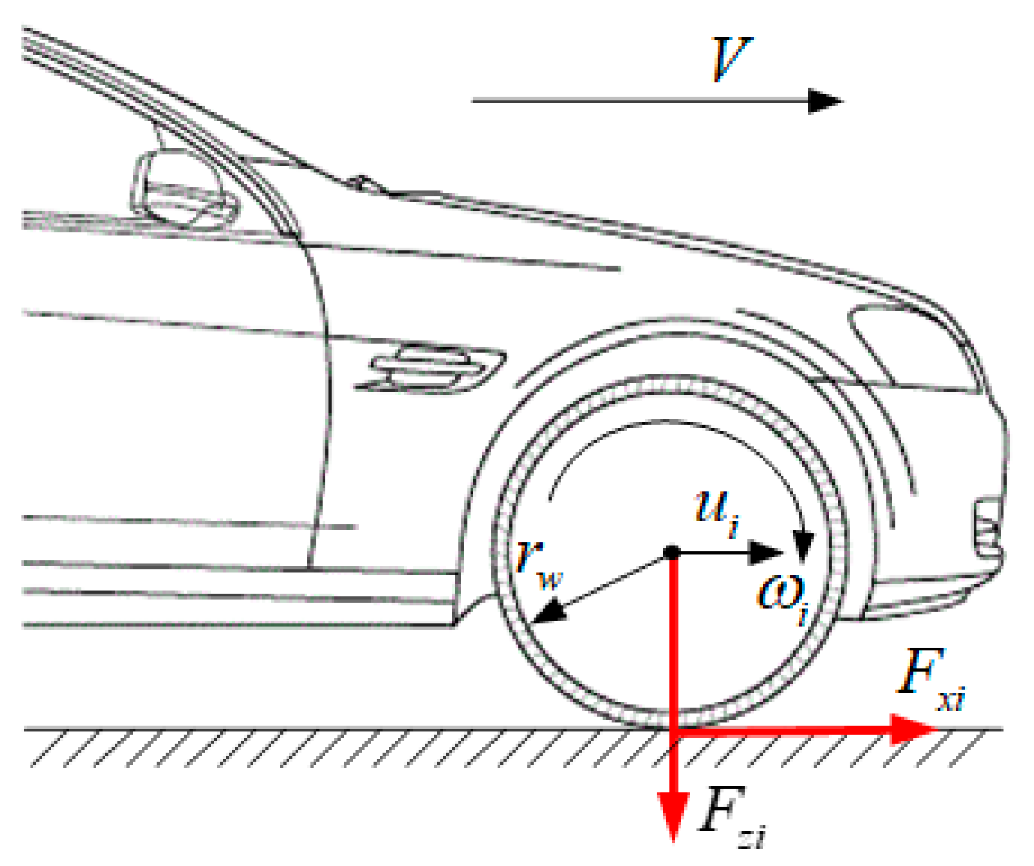
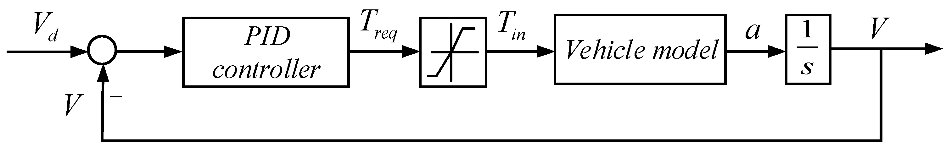
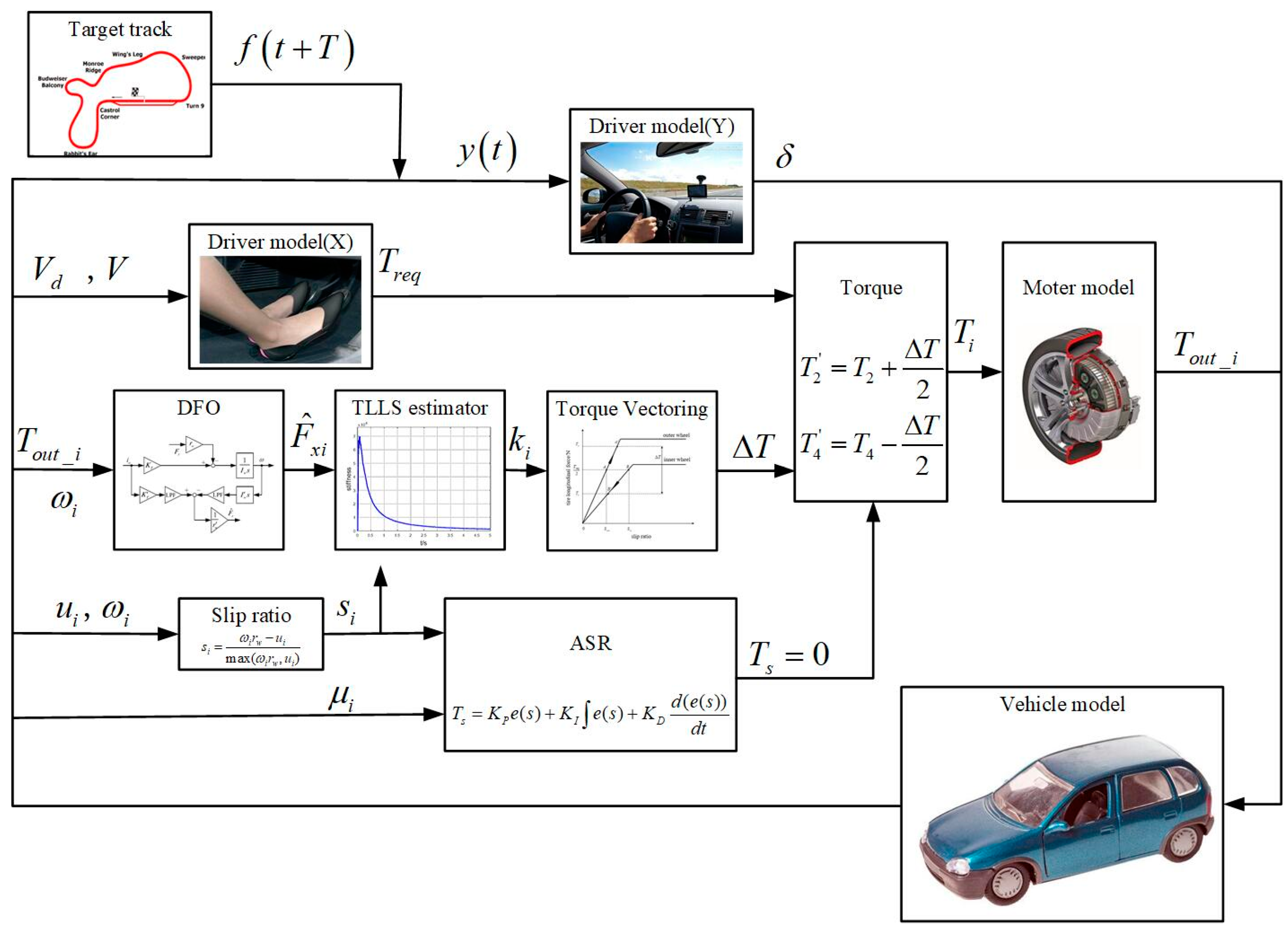
4. Vehicle Model and Torque Vectoring Control Strategy

4.1. Vehicle Model

Figure 4 illustrates the ground forces acting on a seven degrees of freedom (7-DOF) vehicle dynamic model while cornering.

$$m\left(\dot{u}-v{\omega }_r\right)=F_{x1}cos{\delta }_o+F_{x3}cos{\delta }_i-F_{y1}sin{\delta }_o-F_{x3}sin{\delta }_i+F_{x2}+F_{x4}-F_w$$

(16)

$$m\left(\dot{v}+u{\omega }_r\right)=F_{y1}cos{\delta }_o+F_{y3}cos{\delta }_i+F_{x1}sin{\delta }_o+F_{x3}sin{\delta }_i+F_{y2}+F_{y4}$$

(17)

$$\begin{array}{l}I{\dot{\omega }}_r=(F_{x1}\cos {\delta }_o-F_{y1}\sin {\delta }_o-F_{x3}\cos {\delta }_i+F_{y3}\sin {\delta }_i+F_{x2}-F_{x4})B/2\\ +(F_{x1}\sin {\delta }_o+F_{y1}\cos {\delta }_o+F_{x3}\sin {\delta }_i+F_{y3}\cos {\delta }_i)l_f-(F_{y2}+F_{y4})l_r\end{array}$$

(18)

where, ${\delta }_i$ and ${\delta }_o$ are the turning angles of the inner front wheel and outer front wheel respectively; $B$ is the wheel track; $v$ is the lateral speed; $u$ is the longitudinal speed; $F_{yi}$ is the lateral force for every wheel. In this paper, the main parameters of the RWID electric vehicle are shown as

Table 1. Main parameters of the rear-wheel independent-drive (RWID) electric vehicle.

Parameter	Unit	Value
m	kg	1300
l	m	2.662
lr	m	1.2247
lf	m	1.4373
B	m	1.4375
I	kg·m2	1808
Iw	kg·m2	1.85
rw	m	0.285

:

4.2. Determination of the Differential Torque

Based on the analysis about the mechanism of torque vectoring and the longitudinal linear stiffness estimated by RLS, the differential torque should be determined to minimize slip energy consumption to decrease the driving axle slip ratio as well.

In order to minimize slip energy consumption derivation, the partial derivative with respect to in Equation (8) is taken as follows:

$$\frac{\partial P_{ws}}{\partial \Delta T}=\frac{{\omega }_{out}\left(T_{req}+\Delta T\right)}{2r_w{k}_{out}}-\frac{{\omega }_{in}\left(T_{req}-\Delta T\right)}{2r_w{k}_{in}}$$

(19)

Therefore, the optimal differential torque is obtained when $\frac{\partial P_{ws}}{\partial \Delta T}=0$:

$$\Delta T=\frac{k_{out}{\omega }_{in}-k_{in}{\omega }_{out}}{k_{out}{\omega }_{in}+k_{in}{\omega }_{out}}{T}_{req}$$

(20)

Therefore, the torques of two driving wheels can be calculated by Equation (3).

4.3. Torque Vectoring Control Strategy

When the vehicle runs stably and safely, the driver can launch the torque vectoring control. Therefore, acceleration slip regulation (ASR) based on the optimal slip ratio estimation [28] is served as an underlying control for the whole torque vectoring control proposed in this paper.

The longitudinal driver model must enable the vehicle model to follow the target vehicle speed. Therefore, a commonly-used target vehicle speed following longitudinal driver model which is based on Proportional-Integral-Differential (PID) control is established [29], which is shown in Figure 5.

Then the total required torque $T_{req}$ can be calculated by Equation (21).

$$T_{req}=K_{P}e(V)+K_I{\displaystyle \int e(V)}+K_D\frac{\mathrm{d}(e(V))}{\mathrm{d}t}$$

(21)

where, $e(V)$ is the difference between the target vehicle speed and the actual vehicle speed, can be calculated by this equation, $e(V)=V_d-V$; $K_P$, $K_I$ and $K_I$ is the proportional, integral and differentials gains.

This paper ignores the influence of motor efficiency, and simplifies the relationship between the actual output torque $T_{out}$ of the in-wheel motor and the target output torque$T_{out}^{*}$ into a second-order transfer function of the following form:

$$G\left(s\right)=\frac{T_{out}}{T_{out}^{*}}=\frac{1}{a_1{s}^2+a_{2}s+1}$$

(22)

where, $a_1$ and $a_2$ is related to the electromagnetic parameters of the motor.

When the vehicle turns stably and safely and the output of ASR is zero, the torque vectoring control system will start at once. Firstly, DFO continuously outputs the observed longitudinal force of the driving wheels according to the motor torque $T_{motor\_i}$ and wheel rotation speed ${\omega }_i$. At the same time, the tire slip ratio of each wheel is calculated. Next, the longitudinal linear stiffness begins to be estimated based on RLS using the observed longitudinal force and tire slip ratio. Then, the torque vectoring control system starts to work for minimizing slip energy consumption and a crucial differential torque is obtained. The torque for every driving wheel is finally calculated by Equation (3). Then, related instructions are sent to each motor controller to output the respective torque to drive the vehicle cornering. The 7-DOF vehicle dynamic model and the longitudinal driver model was built in MATLAB/Simulink (MathWorks, Natick, MA, USA) [28]. The code of the estimation of TLLS and the control strategy was written in MATLAB. The whole control strategy is shown in Figure 6.

5. Simulation Verification

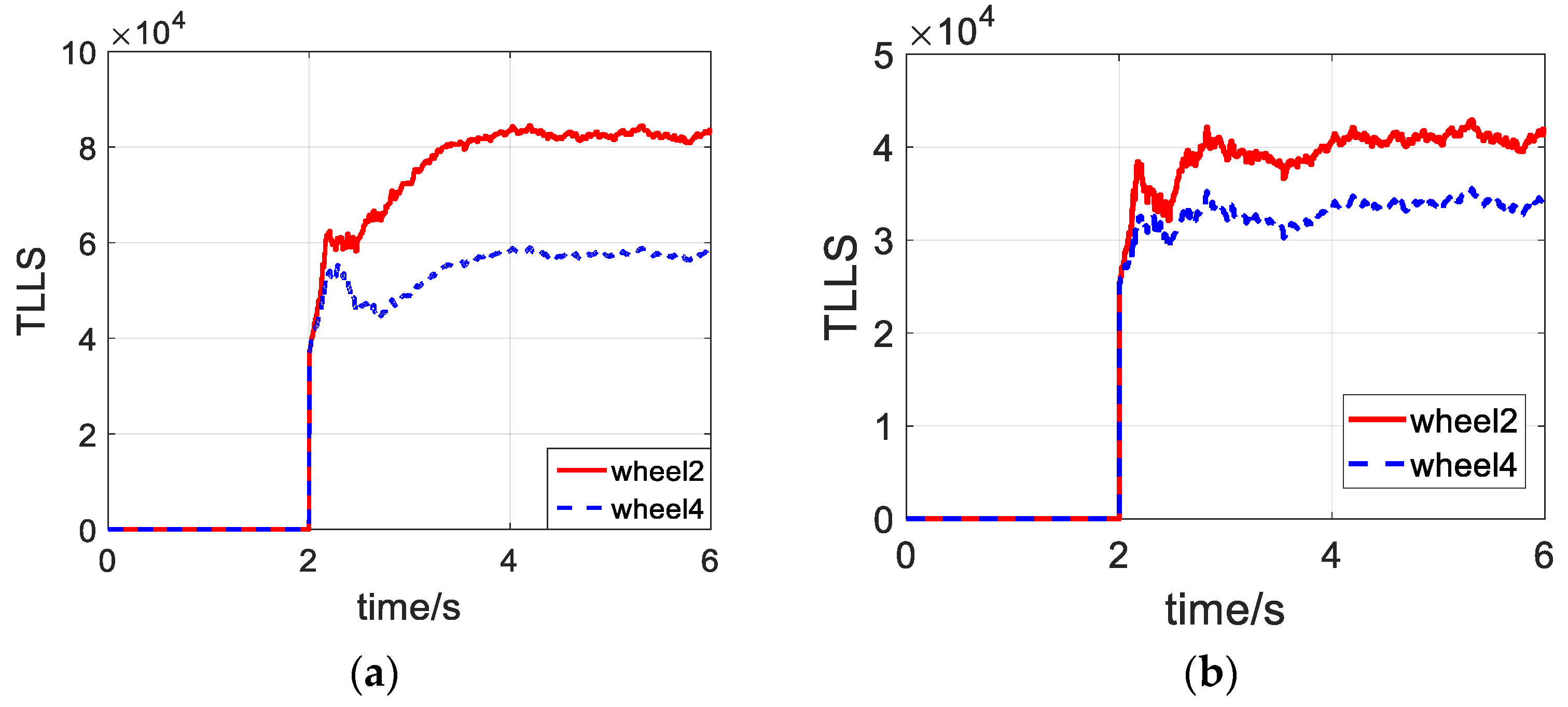
5.1. Verification for Longitudinal Linear Stiffness Estimation

The veracity of longitudinal linear stiffness estimation has been verified by the vehicle model and the tire model. In order to simulate the real observed tire longitudinal force, some white noise is added into the theoretical one. To verify the accuracy of the online estimation result, the normal load, slip ratio and the side slip angle of the two tires, during last 2 s in online simulation are input to the Magic Formula tire model [21].

In the estimation of TLLS, the size of the forgetting factor λ reflects the degree of selection of the data at the previous time. The convergence rate is dependent on the forgetting factor. In our research, in order to verify the convergence rate, we set up λ = 0.94 or λ = 0.98. The result is shown in Figure 7.

It can be seen that the estimation will converge about 0.5 s when λ = 0.94. When λ = 0.98, due to inherit more previous data in the estimation process, the convergence rate is lower. Therefore, in the following simulation, we adopted λ = 0.94.

The following is the simulation verification in a high adhesion coefficient road and low adhesion coefficient road, respectively. The signal sampling rate was 0.01 s which was the same as the sampling rate of vehicle control unit. The vehicle initial speed was set to 60 km/h in the high adhesion coefficient road and 40 km/h in the low adhesion coefficient road and after 2 s of steady running, a step steering angle was input. The online simulation results are as follows. It can be seen in Figure 8a that the linear longitudinal stiffnesses of wheel 2 and wheel 4 are 8.42 × 10⁴ and 5.98 × 10⁴, respectively. In Figure 8b, the linear longitudinal stiffnesses of wheel 2 and wheel 4 are 4.11 × 10⁴ and 3.45 × 10⁴, respectively.

It can be seen in Figure 9 that since tire longitudinal force increases with tire slip ratio increasing and the initial estimation value is pretty small, the estimated TLLS increases fast at first. However, with the instantaneous tire longitudinal force getting close to the peak and the instantaneous tire slip ratio still increasing quickly, the estimated TLLS will decline at once. Therefore, the peak values in Figure 9 are the target TLLS of the two driving wheels, respectively.

On a high adhesion road, the offline estimation results of wheel 2 and wheel 4 are 8.18 × 10⁴ and 5.58 × 10⁴. The estimation errors of the tests above are 2.9% and 1.7%, respectively. On the low adhesion road, the offline estimation results of wheel 2 and wheel 4 are 3.94 × 10⁴ and 3.32 × 10⁴. The estimation errors of the tests above are 4.3% and 3.9%, respectively, which are within the permissible range. This means the estimation results are comparatively accurate and the estimation method for TLLS can be applied to the vehicle.

5.2. Verification for Torque Vectoring Control Strategy

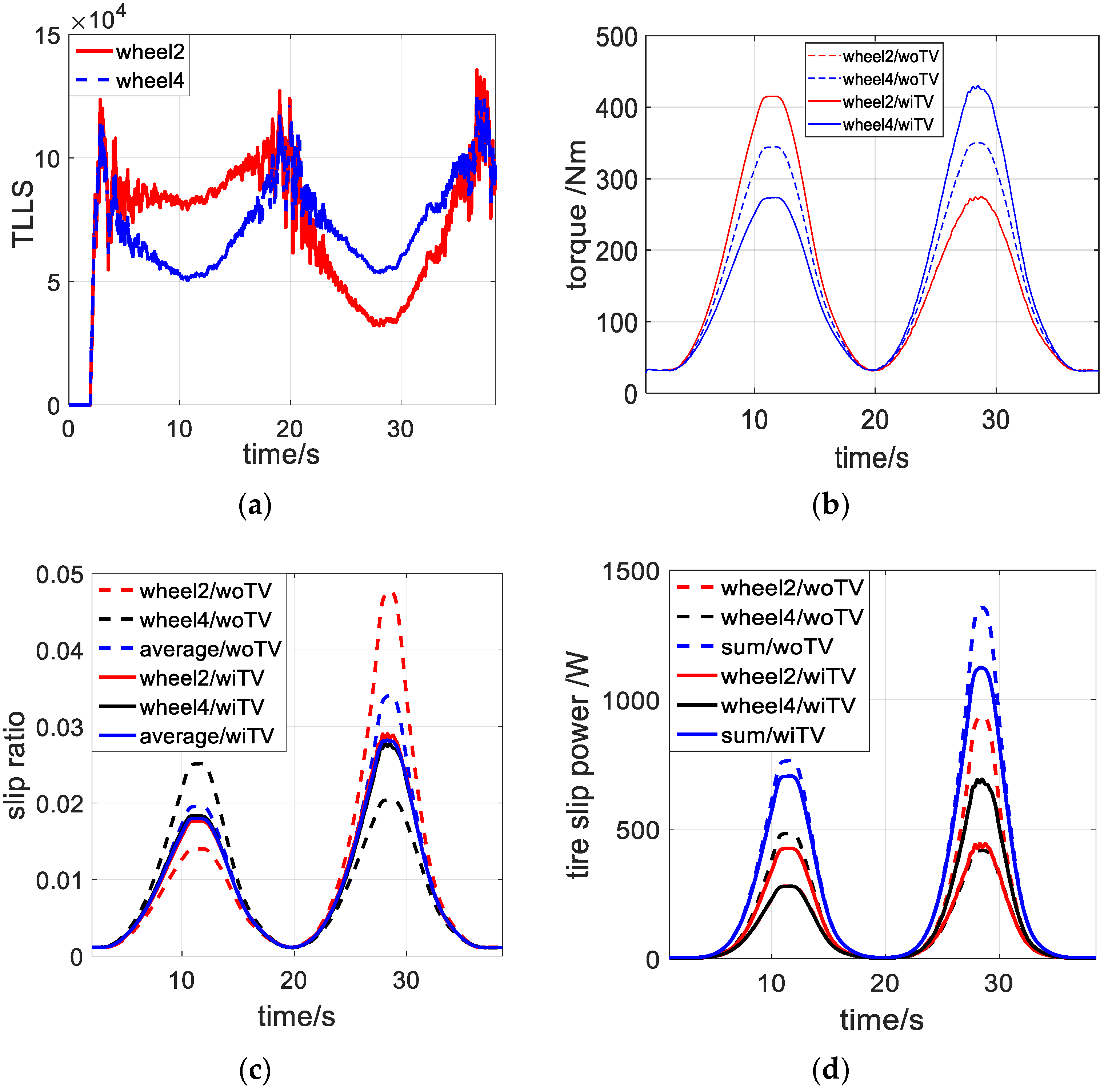
5.2.1. Lemniscate-Shape Path Following

The vehicle’s target speed is set to 60 km/h and after 2 s of steady running, the vehicle enters a lemniscate road, as shown in Figure 10. After running a lip, the vehicle runs out along the tangent of the road.

Figure 10 illustrates the real tracks of the vehicle with and without TV control as well as the target track. It can be seen that, because of an extra yaw moment working on the vehicle and an increased yaw speed, the track with TV control moves slightly closer to the target one, and the controlled vehicle decreases the trend of the understeer characteristic.

During the simulation, the longitudinal linear stiffnesses and driving wheel torque of the vehicle are recorded as shown in Figure 11a,b, and the slip ratio and the slip power consumption of the vehicle with and without TV control are compared in Figure 11c,d.

Figure 11a shows that, with the vehicle turning left, wheel 2 is the outer one, so that it has a higher longitudinal linear stiffness than the inner wheel. Finally, the vehicle runs straight along the tangent of the road, and the normal load of the two tires are equal. Therefore, the identified linear longitudinal stiffness curves of the two tires coincide. The torque of wheel 2 increases and the other one decreases under the effect of the differential torque based on longitudinal linear stiffness. The result of the rear part is quite the contrary. Figure 11b shows that when the vehicle just enters a curve, due to the small steering wheel angle, there is little difference in normal load between the two driving wheels, so the differential torque applied is not very large. As the steering wheel angle and load transfer increases, the difference between the linear longitudinal stiffness of two tires becomes more obvious, and the differential torque applied continues to increase until it reaches a peak value of about 150 Nm around 11 s. In the symmetrical road section, the changes in the driving process are same. Finally, when the vehicle drives straight out, the linear longitudinal stiffness of two tires is equal without steering wheel angle input. The torque vectoring control was no longer performed and the differential torque is zero.

Figure 11c shows that during the front part, the slip ratio of wheel 2 increases and the other one decreases. As a result, the average slip ratio of the rear axle decreases a lot. Therefore, the wear of the tire is comparatively depressed. Compared to the same trend of variations one without TV control, the total power of slip energy consumption has been cut. As for the rear part, the slip ratios of the driving wheels are both higher, and that is why the longitudinal linear stiffness seems lower than that of the front part in Figure 11a. Figure 11d shows that the longitudinal slip energy consumption of the outer driving wheel increases and the inner one decreases. Since the increase in the longitudinal slip energy consumption of the outer drive wheel is less than the amount of reduction, the overall tire longitudinal slip energy consumption is reduced. Ultimately, after calculating, the most reduction of the average rear axle slip ratio is about 17.97% around 28.5 s and the total tire longitudinal slip energy consumption is 227.27 W, about 17.29% lower than that without control.

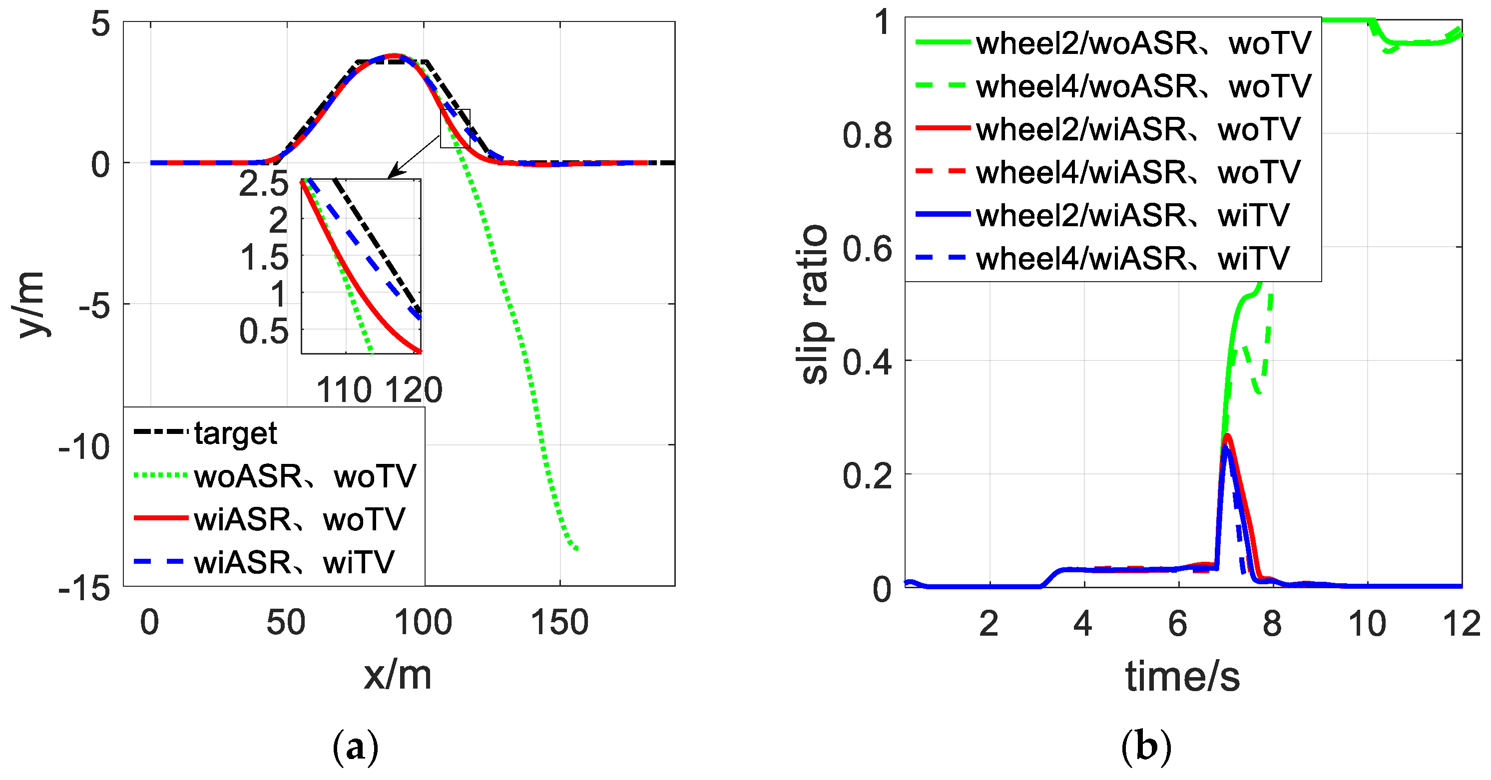
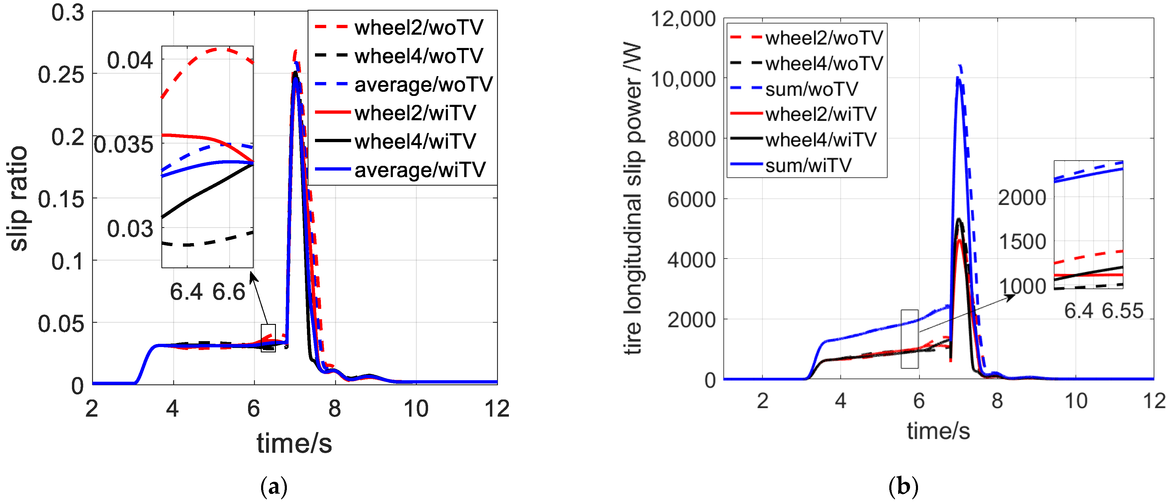
5.2.2. Double Lane Change Maneuvering

The vehicle enters the path at a constant speed of 35 km/h and accelerates at 3 s and keeps the acceleration rate until the vehicle speed reaches 70 km/h. In order to test the ASR system, the maximum coefficient of road adhesion changes suddenly from 0.78 to 0.34 at 6.8 s to ensure that certain driving wheels absolutely slip.

To verify the performances of the proposed control strategy, three kinds of double lane change maneuvering simulation are performed. The first case is that the driver steers the vehicle to complete double lane change maneuvering without ASR and torque vectoring control, which is defined as “woASR, woTV”. The second case, with only ASR working during driving, is defined as “wiASR, woTV”. The third case is in the condition of both of the two-control system working during driving, which is defined as “wiASR, wiTV”. All of the three cases are along with the same maneuvering.

The comparative simulation results of the three cases are shown from Figure 12.

As shown in Figure 12, only the vehicle without ASR has not accomplished the presupposed double lane change maneuvering. The tire slip ratio rockets as the road changes, but with ASR, tire slip ratio falls back to normal later. This means the ASR system ensures the stability of the vehicle even when the vehicle turns in a smooth road suddenly, which fully specifies that it is essential and indispensable to add the ASR system to the whole control system.

Further study and comparison have made for the cases of “wiASR, woTV” and “wiASR, wiTV” so that the function of torque vectoring control can be illustrated clearly. Figure 13 describes the calculated differential torque while the vehicle turns.

For the first few seconds, the vehicle turns in a road with good adhesion and there is no driving wheel slipping. Torque vectoring control starts at 3 s and a differential torque shown in Figure 13 is applied on the driving wheels. First, the vehicle turns to the left, wheel 2 is the outer wheel, and wheel 4 is the inner wheel. A positive differential torque is applied between the driving wheels, and the peak value is about 39 Nm. Subsequently, the driver’s input to the steering wheel continues to decrease and gradually begins to turn to the right. A negative differential torque is applied between the driving wheels and as the lateral load transfer of the vehicle increases, the differential torque reaches the peak value again of about 85 Nm. However, since the sudden change of the road at 6.8 s, the tires slipping tumultuously, and the stability of vehicle turns into the first aim. As a result, ASR has to start immediately and at the same time torque vectoring control secedes until a friendly relationship between tire and road is established again. Therefore, the differential torque is zero within some time.

The slip ratio and tire longitudinal slip energy consumption are shown in Figure 14.

By calculating, when the vehicle with torque vectoring control runs stably (3~6.8 s), the rear driving axle average slip ratio decreases distinctly and the maximum reduction is about 2.97% at 6.6 s. As shown in Figure 14, the total tire longitudinal slip energy consumption decreases due to the differential torque. Regardless of the slipping process, the tire longitudinal slip power decreases distinctly and the maximum reduction is 73.95 W which is about 3.08% of the tire longitudinal slip power of the vehicle without torque vectoring control. During the whole cornering process, the total tire longitudinal slip energy consumption decreases by 16.12 W for about 0.77%.

6. Conclusions

In this paper, the mechanism of torque vectoring for reducing total tire slips in a driving axle is analyzed. An overall torque vectoring control method with anti-slip regulation for minimizing slip energy consumption based on the tire longitudinal linear stiffness is proposed. With the help of the fast and accurate estimation of the longitudinal linear stiffness, the differential torque between the two side of driving wheels can be determined. The simulation results show that, by the appropriate differential torque applied to the driving wheels based on the tire linear longitudinal stiffness estimation, the average rear axle slip ratio decreases, which represents the reduction in the wear of the tire. More importantly, the tire slip energy consumption decreased 17.29% in following a lemniscate-shaped path, and decreased 0.77% in the double lane change maneuvering simulation when the slip ratio decreased. Although the energy saving rate was not huge, taking long-range driving into consideration, especially on urban roads or rural hill roads with many corners, the final total energy-saving data cannot be ignored. That is to say, the torque vectoring technology has been proven to benefit driving energy efficiency improvement.

References

1. Viola, F. Electric Vehicles and Psychology. Sustainability 2021, 13, 719. [Google Scholar] [CrossRef]
2. Mariusz, I.; Marianna, J. An Efficient Hybrid Algorithm for Energy Expenditure Estimation for Electric Vehicles in Urban Service Enterprises. Energies 2021, 14, 2004. [Google Scholar]
3. Gu, J.; Ouyang, M.; Lu, D.; Li, J.; Lu, L. Energy efficiency optimization of electric vehicle driven by in-wheel motors. Int. J. Automot. Technol. 2013, 14, 763–772. [Google Scholar] [CrossRef]
4. Zhang, H.H.; Jin, L.Q.; Wang, Q.N. Simulation of energy-saving driving mode during steering for motorized wheels driving vehicle. J. Traffic Transp. Eng. 2010, 4, 42–46. [Google Scholar]
5. Koehler, S.; Viehl, A.; Bringmann, O.; Rosenstiel, W. Improved Energy Efficiency and Vehicle Dynamics for Battery Electric Vehicles through Torque Vectoring Control. In Proceedings of the IEEE Intelligent Vehicles Symposium, Seoul, Korea, 28 June–1 July 2015; pp. 749–754. [Google Scholar]
6. Pennycott, A.; Novellis, L.D.; Sorniotti, A.; Gruber, P. The Application of Control and Wheel Torque Allocation Techniques to Driving Modes for Fully Electric Vehicles. SAE Int. J. Passeng. Cars Mech. Syst. 2014, 17, 488–496. [Google Scholar] [CrossRef]
7. Pierpaolo, P.; Ivan, A.; Cesare, P. Optimal Energy Management for Hybrid Electric Vehicles Based on Dynamic Programming and Receding Horizon. Energies 2021, 14, 3502. [Google Scholar] [CrossRef]
8. Kobayashi, T.; Katsuyama, E. Efficient Direct Yaw Moment Control: Tyre Slip Power Loss Minimisation for Four-Independent Wheel Drive Vehicle. Int. J. Veh. Mech. Mobil. 2018, 56, 719–733. [Google Scholar] [CrossRef]
9. Himeno, H.; Katsuyama, E.; Kobayashi, T. Efficient Direct Yaw Moment Control during Acceleration and Deceleration While Turning. SAE 2016 World Congress and Exhibition. Available online: https://saemobilus.sae.org/content/2016-01-1677/ (accessed on 5 April 2016).
10. Sun, W.; Rong, J.; Wang, J.; Zhang, W.; Zhou, Z. Research on Optimal Torque Control of Turning Energy Consumption for EVs with Motorized Wheels. Energies 2021, 14, 6947. [Google Scholar] [CrossRef]
11. Suzuki, Y.; Kano, Y.; Abe, M. A study on tire force distribution controls for full drive-by-wire electric vehicle. Veh. Syst. Dyn. 2014, 52, 235–250. [Google Scholar] [CrossRef]
12. Wang, Y.; Fujimoto, H.; Hara, S. Driving Force Distribution and Control for EV with Four In-Wheel Motors: A Case Study of Acceleration on Split-Friction Surfaces. IEEE Trans. Ind. Electron. 2017, 64, 3380–3388. [Google Scholar] [CrossRef]
13. Maeda, K.; Fujimoto, H.; Hori, Y. Four-wheel driving-force distribution method based on driving stiffness and slip ratio estimation for electric vehicle with in-wheel motors. In Proceedings of the IEEE Vehicle Power and Propulsion Conference, Seoul, Korea, 9–12 October 2012. [Google Scholar]
14. Wang, J.; Gao, S.; Wang, K.; Wang, Y.; Sun, W.; Wang, Q. Wheel torque distribution optimization of four-wheel independent-drive electric vehicle for energy efficient driving. Control Eng. Pract. 2021, 110, 1–14. [Google Scholar] [CrossRef]
15. Lin, C.; Xu, Z. Wheel Torque Distribution of Four-Wheel-Drive Electric Vehicles Based on Multi-Objective Optimization. Energies 2015, 8, 3815–3831. [Google Scholar] [CrossRef] [Green Version]
16. Dieckmann, T. Assessment of Road Grip by Way of Measured Wheel Variables. In Proceedings of the FISITA, London, UK, 7–11 June 1992. [Google Scholar]
17. Gustafsson, F. Slip-Based Estimation Of Tire-Road Friction. Automatica 2013, 33, 1087–1099. [Google Scholar] [CrossRef]
18. Ikushima, Y.; Sawase, K. A Study on the Effects of the Active Yaw Moment Control. In Proceedings of the International Congress & Exposition, Detroit, MI, USA, 1 February 1995. [Google Scholar]
19. Sun, W.; Wang, J.; Wang, Q.; Assadian, F.; Fu, B. Simulation investigation of tractive energy conservation for a cornering rear-wheel-independent-drive electric vehicle through torque vectoring. Sci. China Technol. 2018, 61, 257–272. [Google Scholar] [CrossRef]
20. Isermann, R. Fahrdynamik-Regelung: Modellbildung, Fahrerassistenzsysteme, Mechatronik; Vieweg: Wiesbaden, Germany, 2006. [Google Scholar]
21. Pacejka, H.B. Tire and Vehicle Dynamics; Butterworth Heinemann: Oxford, UK, 2012. [Google Scholar]
22. Ahn, C.; Peng, H.; Tseng, H.E. Robust Estimation of Road Frictional Coefficient. IEEE Trans. Control Syst. Technol. 2012, 21, 1–13. [Google Scholar] [CrossRef]
23. Yi, K.; Hedrick, K.; Lee, S. Estimation of Tire-Road Friction Using Observer Based Identifiers. Veh. Syst. Dyn. 2010, 31, 233–261. [Google Scholar] [CrossRef]
24. Miller, S.L.; Youngberg, B.; Millie, A.; Schweizer, P.; Gerdes, J.C. Calculating Longitudinal Wheel Slip and Tire Parameters Using GPS Velocity. In Proceedings of the IEEE Proceedings of the American Control Conference, Arlington, VA, USA, 25–27 June 2001. [Google Scholar]
25. Multirate hybrid adaptive control. IEEE Trans. Autom. Control 1986, 31, 582–586. [CrossRef]
26. Haykin, S. Adaptive Filter Theory, 2nd ed.; Wiley: Hoboken, NJ, USA, 2002; Volume 4, pp. 469–490. [Google Scholar]
27. Vahidi, A.; Stefanopoulou, A.; Peng, H. Recursive least squares with forgetting for online estimation of vehicle mass and road grade: Theory and experiments. Veh. Syst. Dyn. 2005, 43, 31–35. [Google Scholar] [CrossRef]
28. Wang, J.; Wang, Q.; Jin, L.; Song, C. Independent wheel torque control of 4WD electric vehicle for differential drive assisted steering. Mechatronics 2011, 21, 63–76. [Google Scholar] [CrossRef]
29. Junya, Y.; Akira, K.; Keiji, W. A method of torque control for independent wheel drive vehicles on rough terrain. J. Terramechanics 2007, 44, 371–381. [Google Scholar]
Figure 1. Longitudinal force characteristics of inner and outer driving wheels.
Energies 14 08143 g001
Figure 2. Simplified tire adhesion curve.
Energies 14 08143 g002
Figure 3. Single driving wheel model.
Energies 14 08143 g003
Figure 4. Seven degrees of freedom (7-DOF) vehicle dynamic mode.
Energies 14 08143 g004
Figure 5. The longitudinal driver model.
Energies 14 08143 g005
Figure 6. The overall diagram of torque vectoring control strategy.
Energies 14 08143 g006
Figure 7. Tire linear longitudinal stiffness (TLLS) with different λ.
Energies 14 08143 g007
Figure 8. TLLS: (a) high adhesion coefficient road; (b) low adhesion coefficient road.
Energies 14 08143 g008
Figure 9. The offline estimation of longitudinal linear stiffness: (a) wheel 2/offline/high adhesion; (b) wheel 4/offline/high adhesion; (c) wheel 2/offline/low adhesion; (d) wheel 4/offline/low adhesion.
Energies 14 08143 g009
Figure 10. Track.
Energies 14 08143 g010
Figure 11. The lemniscate-shape path simulation: (a) TLLS.; (b) torque; (c) the slip ratio; (d) the slip power consumption.
Energies 14 08143 g011
Figure 12. The double lane change maneuvering simulation: (a) track; (b) tire slip ratio.
Energies 14 08143 g012
Figure 13. Differential torque.
Energies 14 08143 g013
Figure 14. The double lane change maneuvering simulation: (a) slip ratio; (b) tire slip power.
Energies 14 08143 g014