
Generation of Realistic Boundary Conditions at the Combustion Chamber/Turbine Interface Using Large-Eddy Simulation


Abstract
1. Introduction
2. Combustion Chamber/Turbine Integrated Simulation
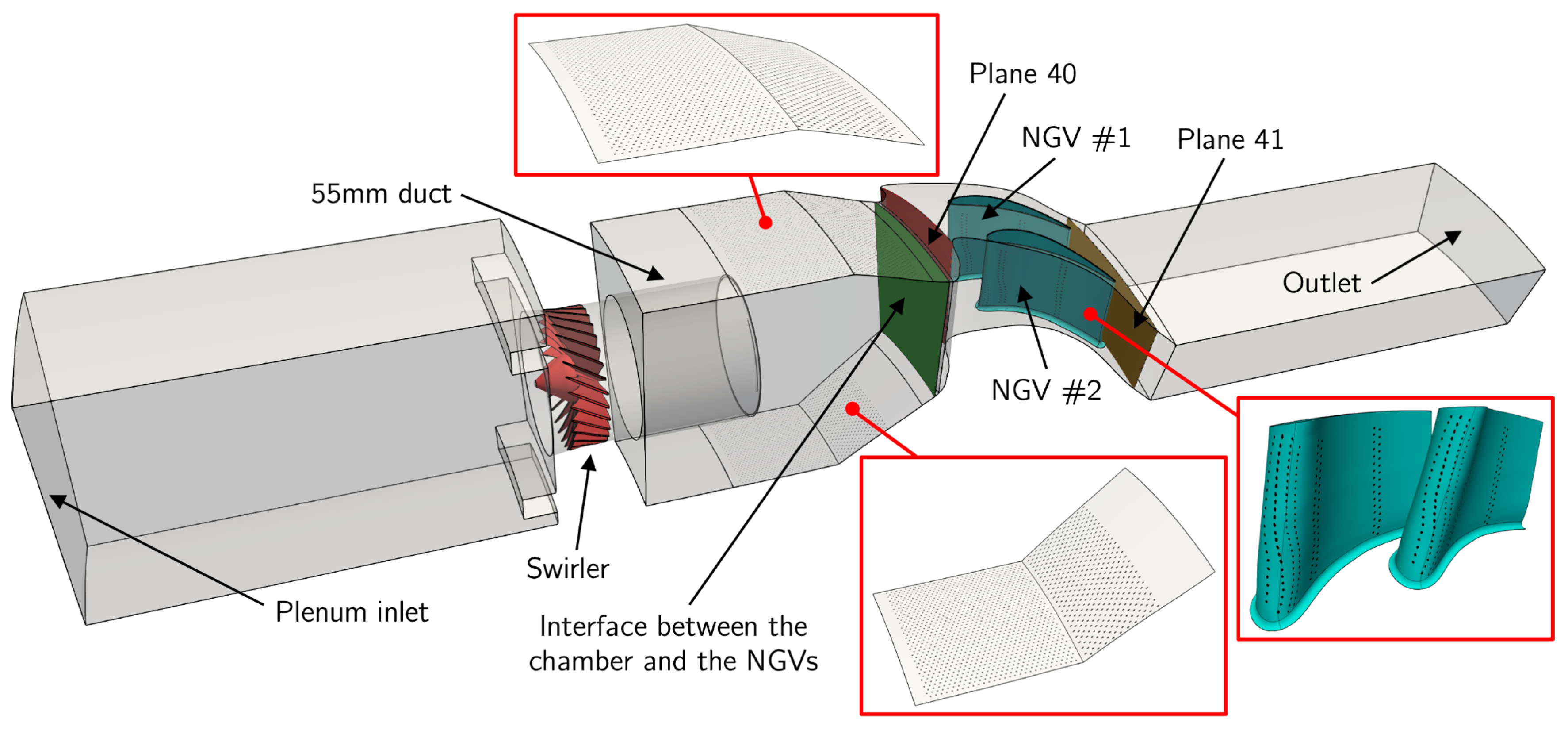
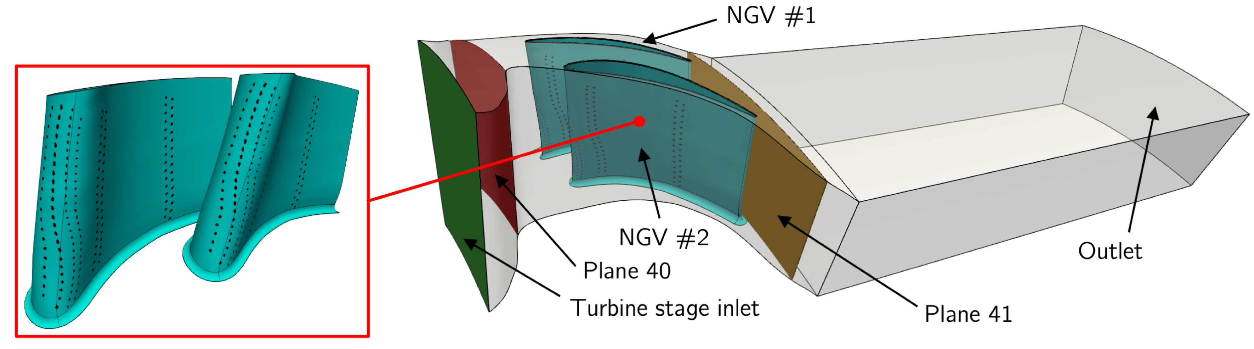
2.1. Description of the Configuration
2.2. Modal Decompositions of the Database
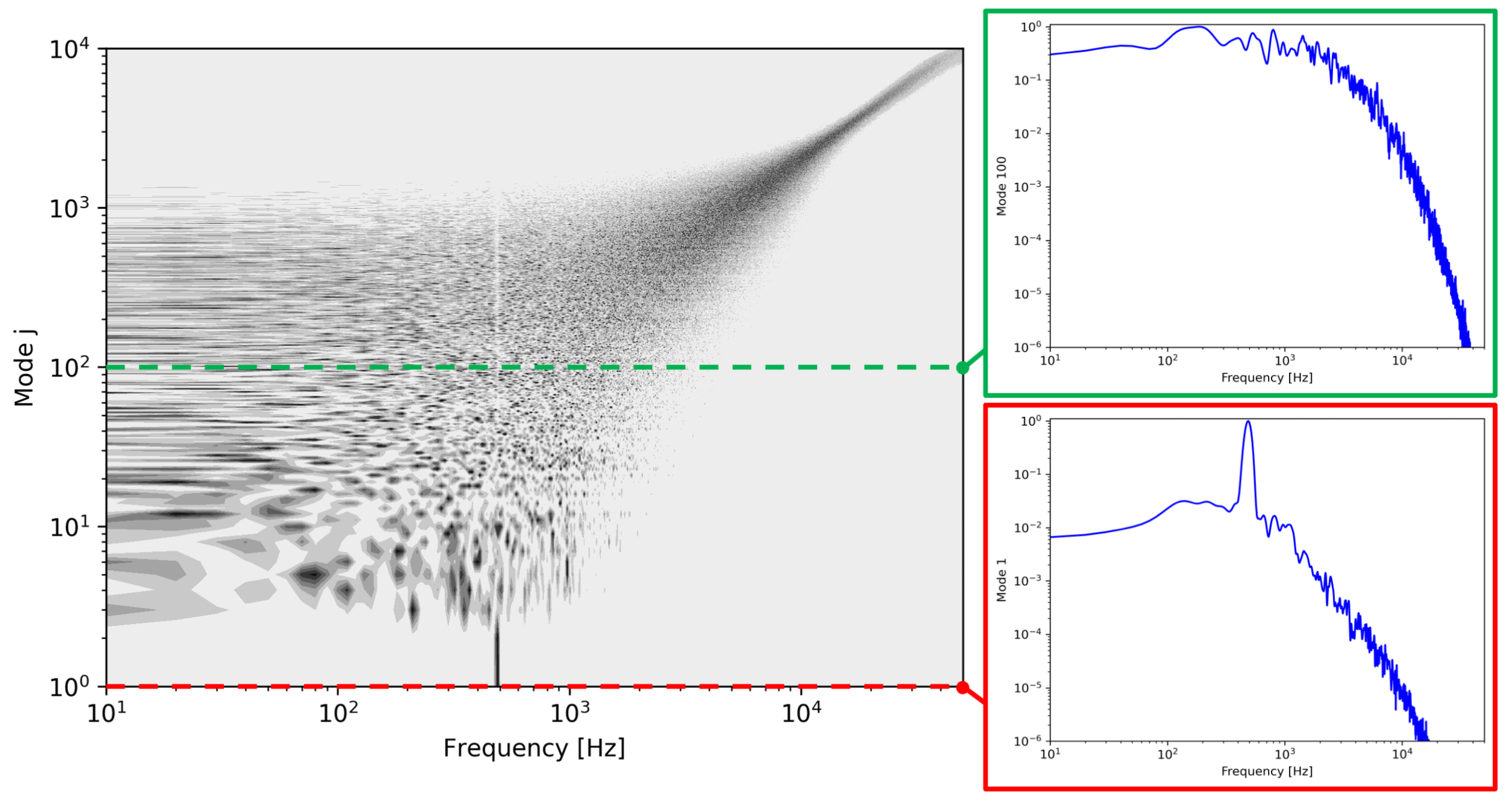
2.2.1. Modal Decomposition 1: Spectral Proper Orthogonal Decomposition (SPOD)
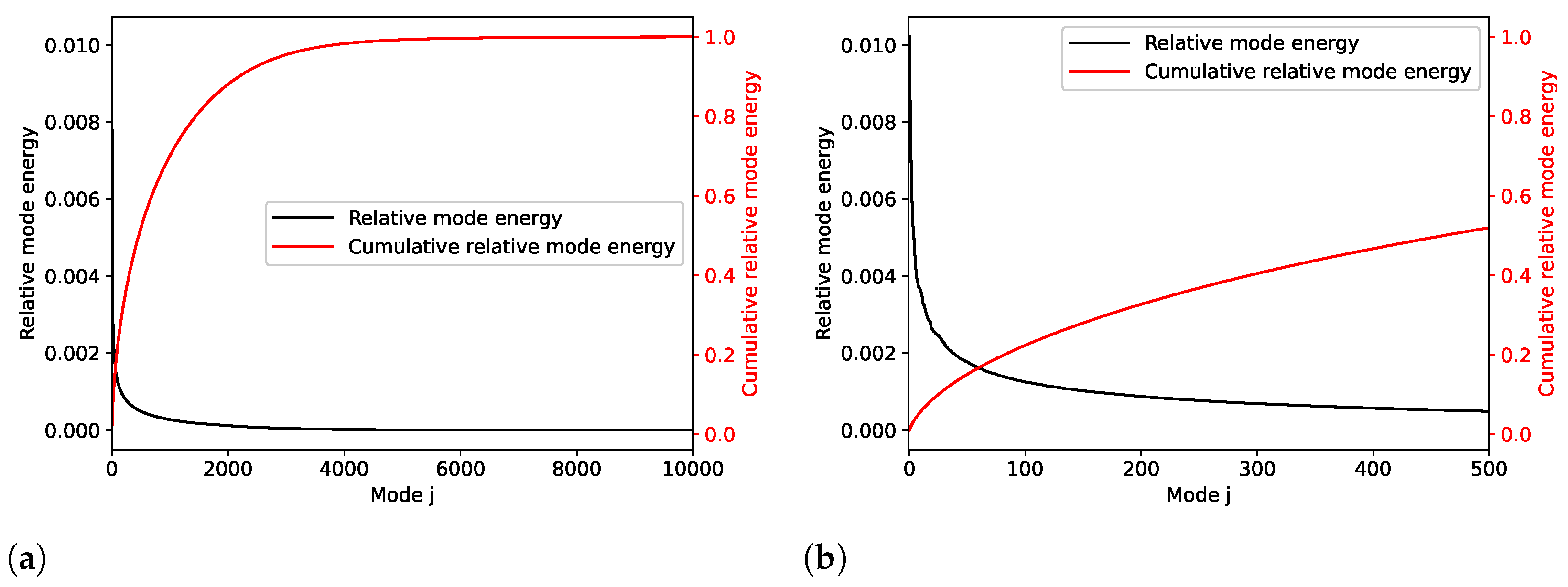
2.2.2. Modal Decomposition 2: Proper Orthogonal Decomposition (POD)
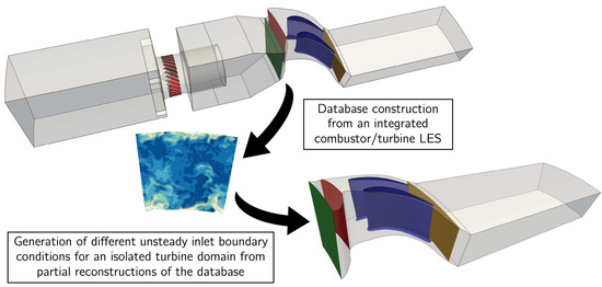
3. Generation of an Unsteady Inlet Boundary Condition for an Isolated Turbine Simulation
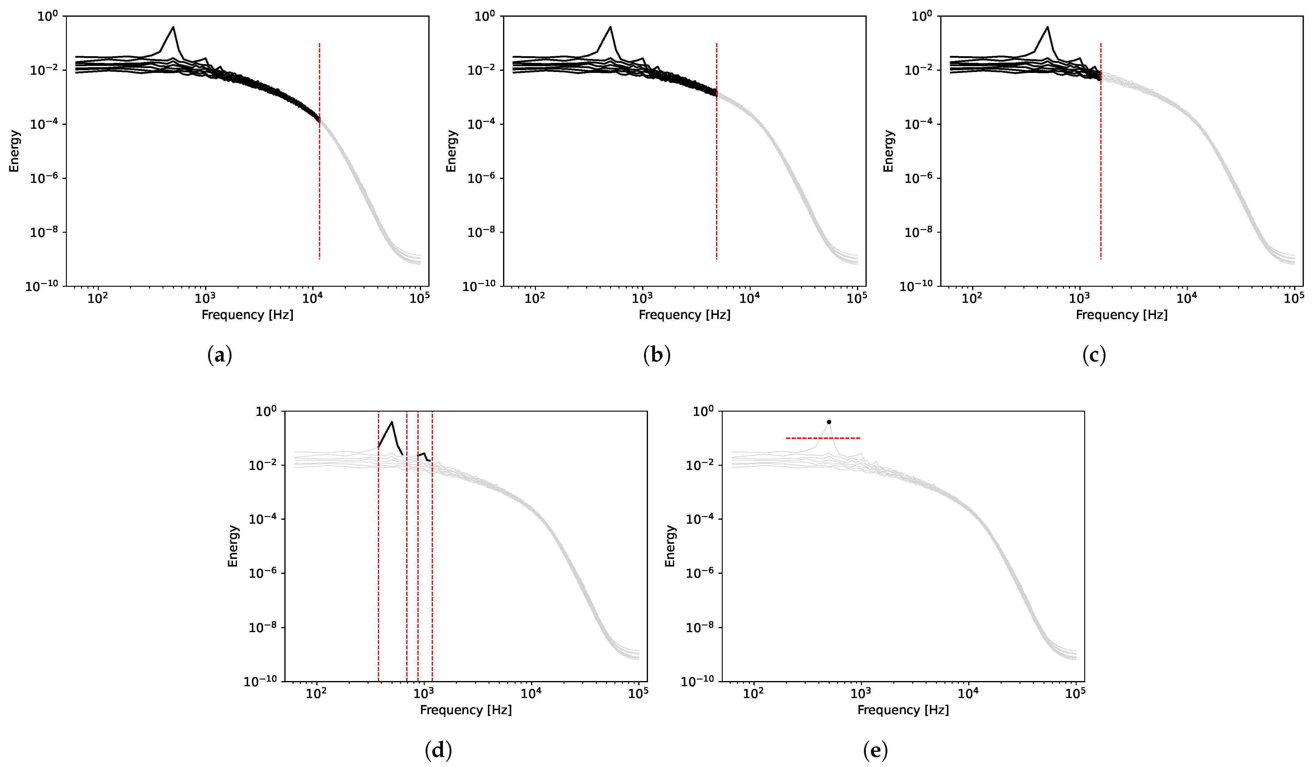
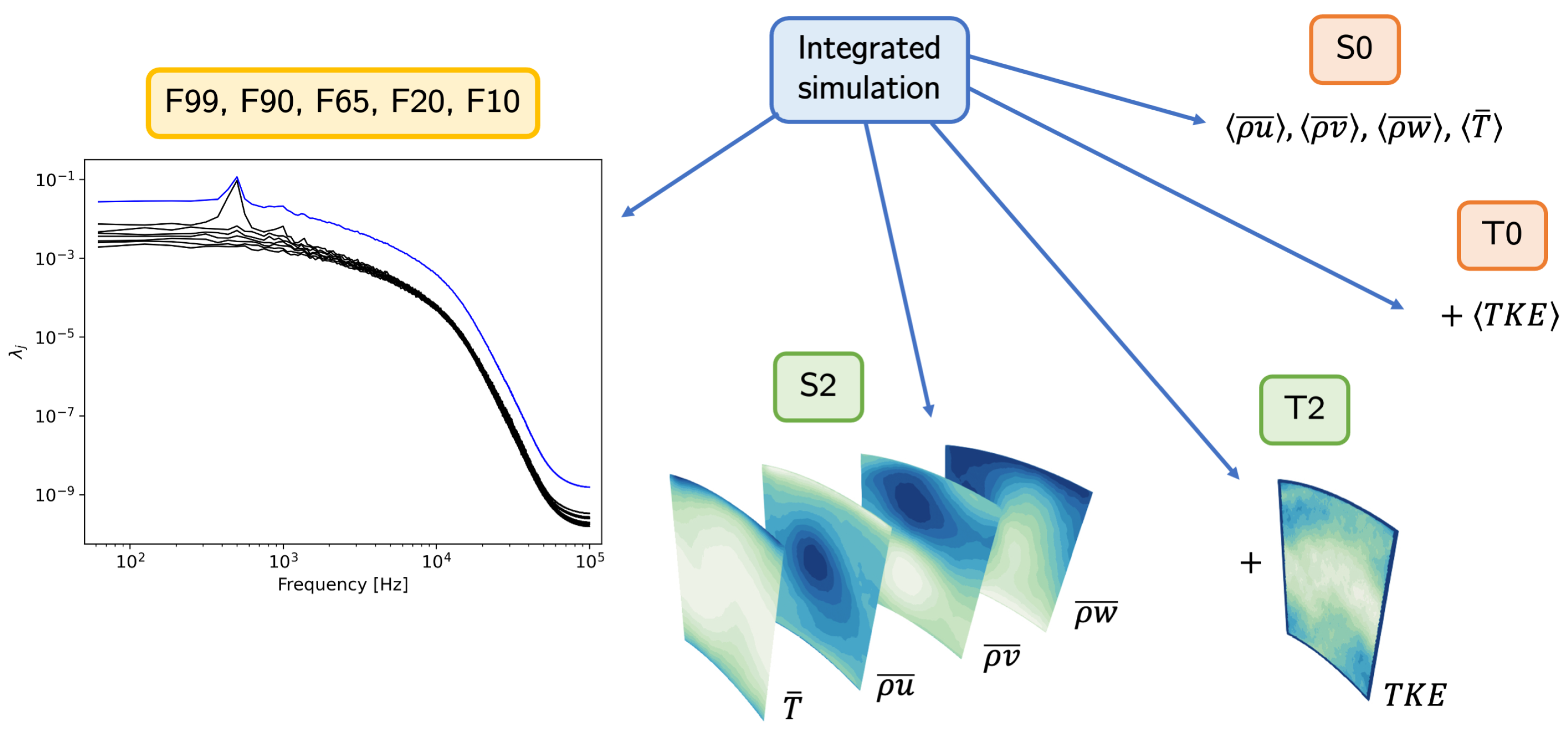
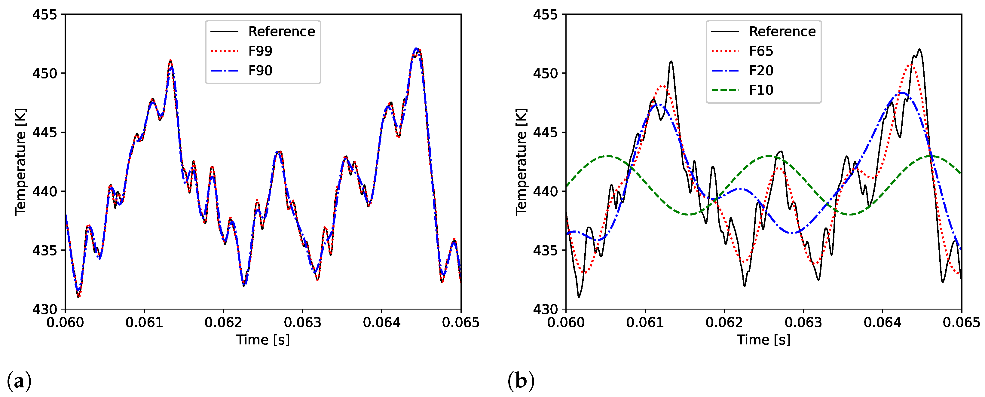
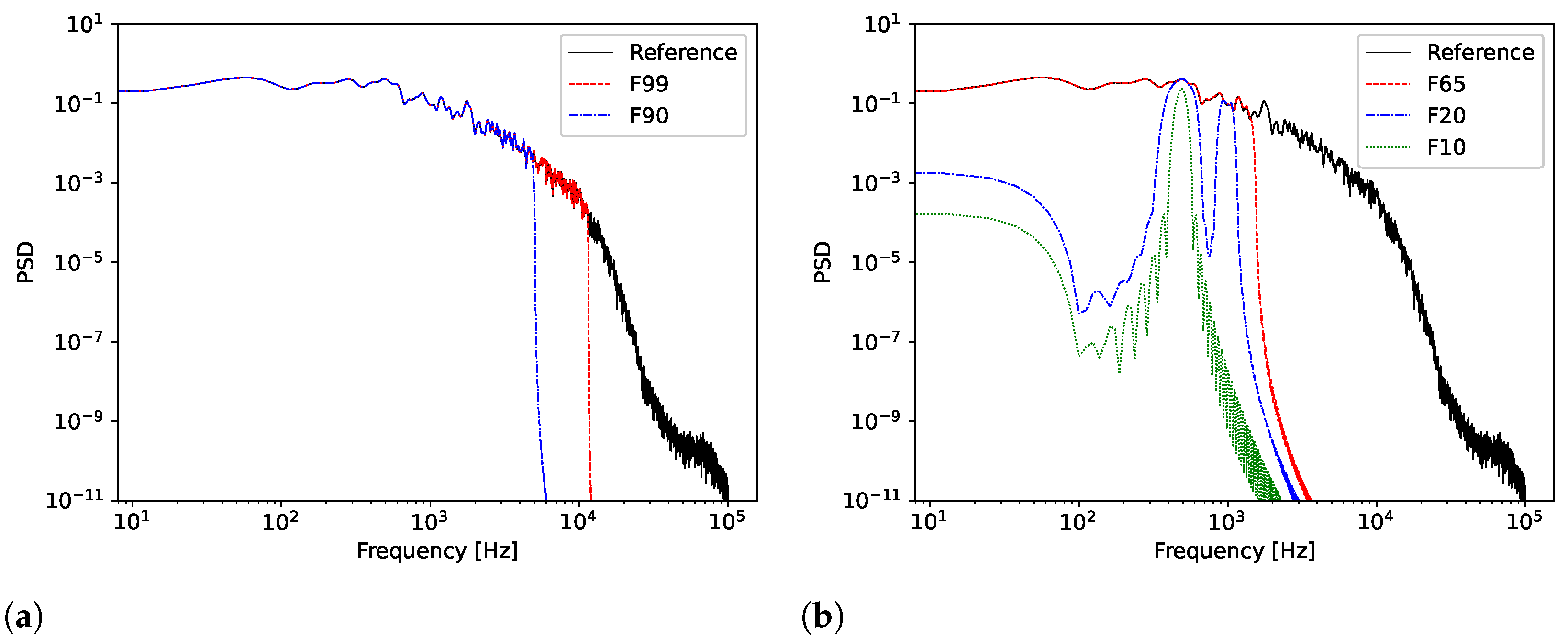
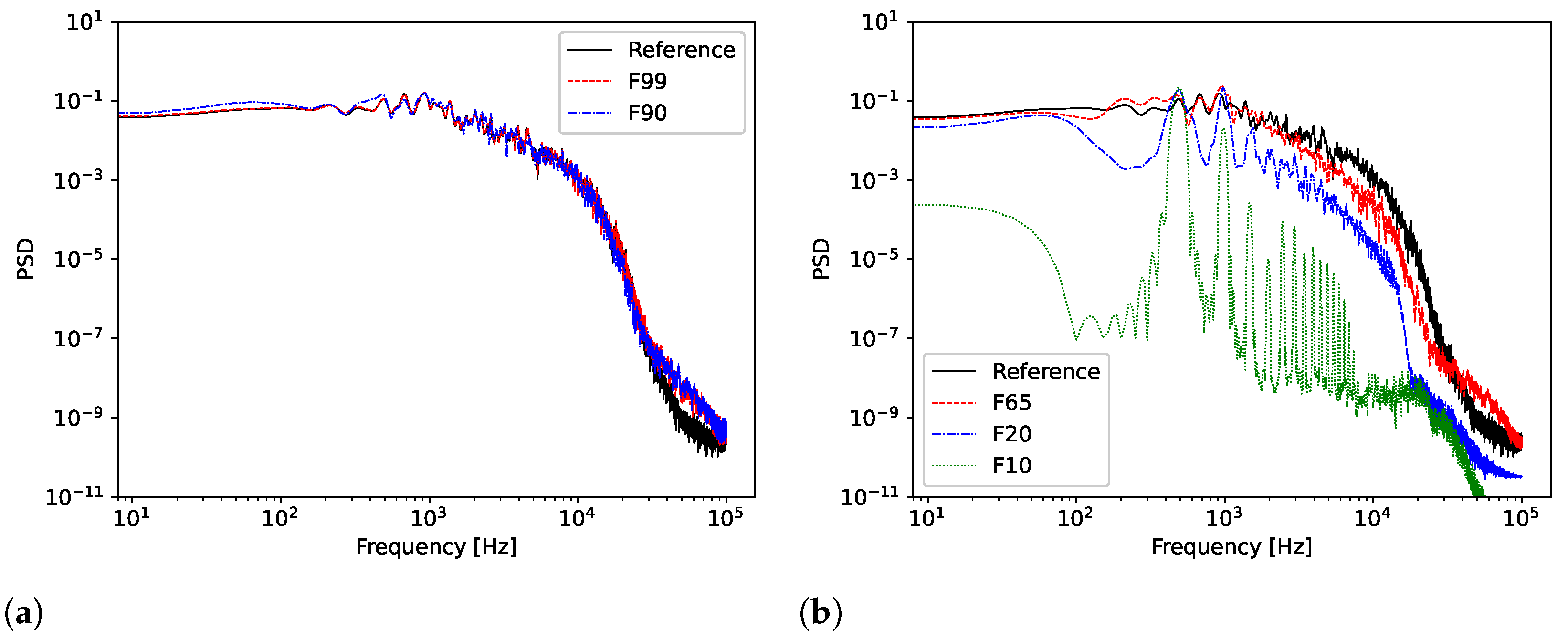
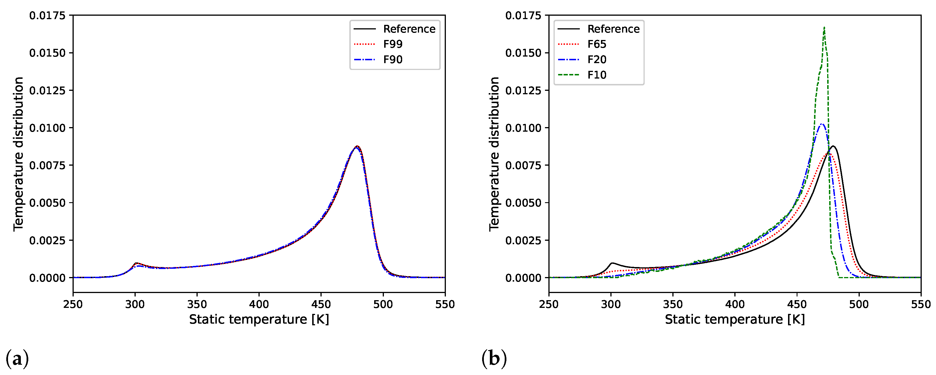
- Case F99 corresponds to a reconstruction containing 99% of the total energy, with all seven identified modes and the first 185 frequencies which extend to 11,500 Hz.
- Case F90 corresponds to a reconstruction containing 90% of the total energy, with, again, the seven modes and the first 79 frequencies which extend to 5000 Hz.
- Case F65 corresponds to a reconstruction containing 65% of the total energy, with the seven modes and the first 26 frequencies which extend to 1500 Hz.
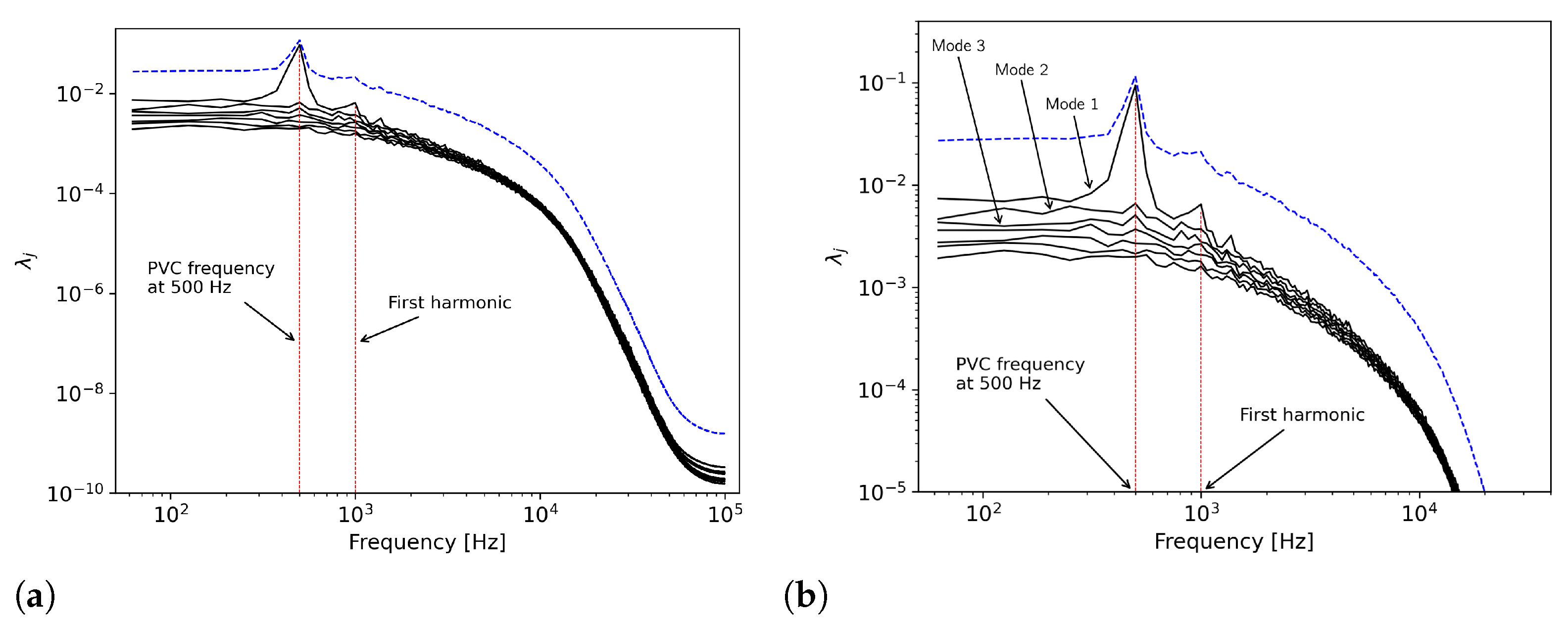
- Case F20 corresponds to a reconstruction containing 20% of the total energy, with only the first mode and the frequencies around 500 Hz, as well as the first harmonic at 1000 Hz.
- Case F10 corresponds to a reconstruction containing 10% of the total energy, with only the first mode and the dominant frequency at 500 Hz (Figure 12).

- Case S0: the inlet boundary condition is imposed by specifying 0D quantities in space and time, i.e., by imposing the three components of momentum , , and and the static temperature (spatially and temporally averaged values of the integrated simulation).
- Case T0: the quantities imposed at the inlet are the same as for case S0, with the addition of velocity fluctuations generated randomly to create turbulent activity in space and time. Turbulence is injected here using the synthetic approach proposed by Guezennec et al. [38] from a Passot–Pouquet spectrum [39]. The velocity fluctuation value used comes from the integrated simulation and the most energetic length scale is specified at , with h the height of the channel. This quantity corresponds to the characteristic size of the most energetic structures of the Passot–Pouquet spectrum [39] (not to be confused with the integral scale which is expressed as ).
- Case S2: the inlet boundary condition is imposed from time-averaged 2D maps at the interface of the integrated simulation for , , , and T. The boundary condition condition is therefore constant in time, but variable in space.
- Case T2: this case is identical to S2 with the addition of a 2D map of velocity fluctuations. The turbulent 2D field coincides with the turbulent kinetic energy at the interface of the integrated simulation, i.e., time-averaged fluctuating field. Unlike the T0 case, the value of the velocity fluctuations used to generate the synthetic turbulence is hence not constant in space. Note that the turbulence injection method does not inject fluctuations on temperature.
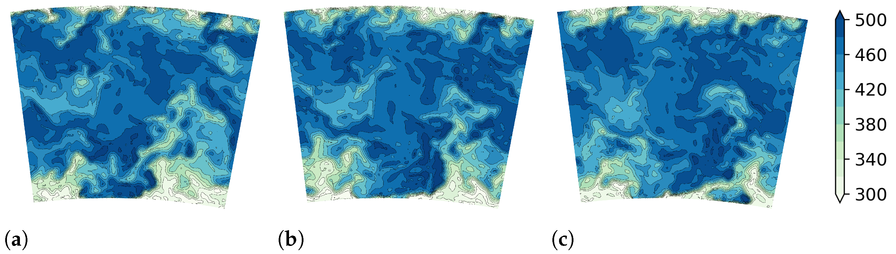
Analysis of the Reconstructed Fields
4. Effects of the Boundary Condition of the Isolated Simulation Predictions
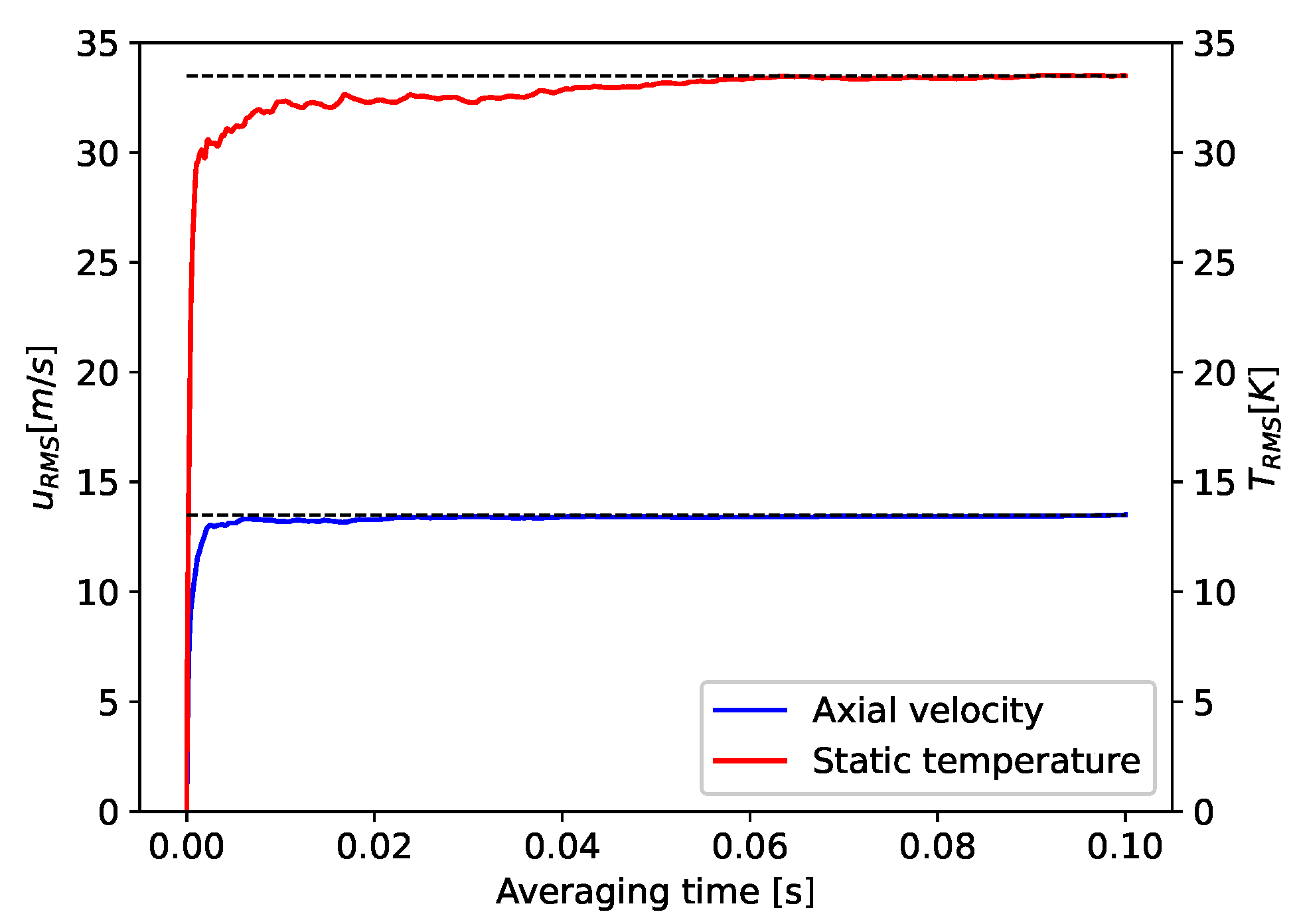
4.1. Turbulent Fluctuations
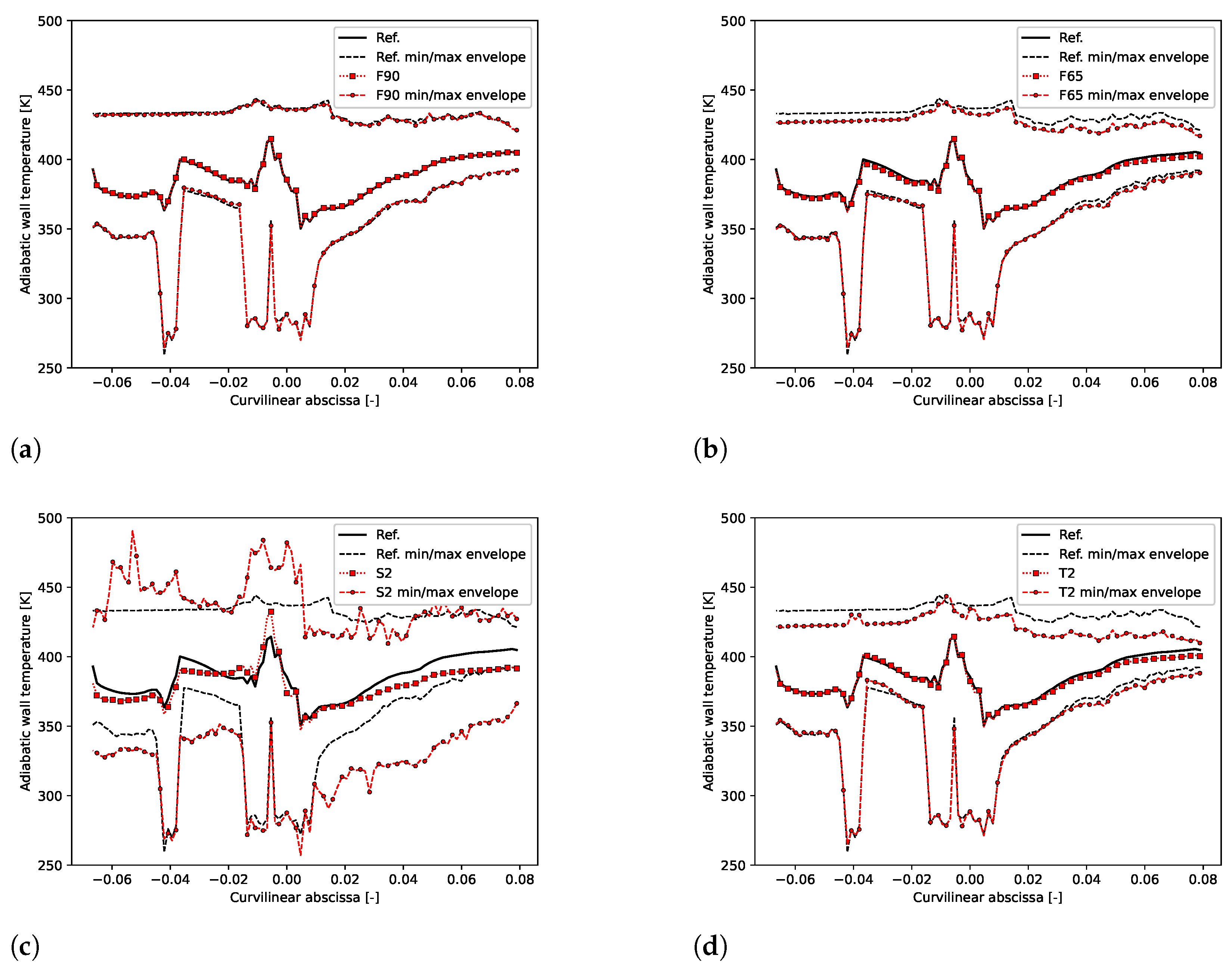
4.2. Adiabatic Wall Temperature
5. Conclusions
Author Contributions
Funding
Institutional Review Board Statement
Informed Consent Statement
Data Availability Statement
Acknowledgments
Conflicts of Interest
Abbreviations
| FACTOR | Full Aero-thermal Combustor-Turbine Interaction Research |
| LES | Large-Eddy Simulation |
| NGV | Nozzle Guide Vanes |
| POD | Proper Orthogonal Decomposition |
| PSD | Power Spectral Density |
| PVC | Precessing Vortex Core |
| RMS | Root Mean Square |
| SPOD | Spectral Proper Orthogonal Decomposition |
| TKE | Turbulent Kinetic Energy |
| Turbulence intensity | |
| L | Turbine mid radius |
| Total pressure | |
| Q | Mass flow rate |
| Reduced mass flow rate | |
| R | Perfect gas constant |
| T | Static temperature |
| Total temperature | |
| Three components of velocity | |
| Eigenvalue | |
| Density | |
| Time-averaged quantity | |
| Temporal fluctuations of a quantity | |
| Spatially-averaged quantity |
References
- Medic, G.; Kalitzin, G.; You, D.; Herrmann, M.; Ham, F.; Weide, E.; Pitsch, H.; Alonso, J. Integrated RANS/LES computations of turbulent flow through a turbofan jet engine. Annu. Res. Briefs 2006, 275–285. Available online: https://web.stanford.edu/group/ctr/ResBriefs06/21_medic1.pdf (accessed on 2 December 2021).
- Medic, G.; You, D.; Kalitzin, G.; Herrmann, M.; Ham, F.; Pitsch, H.; van der Weide, E.; Alonso, J. Integrated Computations of an Entire Jet Engine. In Proceedings of the ASME Turbo Expo 2007: Power for Land, Sea, and Air, Montreal, QC, Canada, 14–17 May 2007; Volume 6, pp. 1841–1847. [Google Scholar] [CrossRef]
- Pérez Arroyo, C.; Dombard, J.; Duchaine, F.; Gicquel, L.; Martin, B.; Odier, N.; Staffelbach, G. Towards the large-eddy simulation of a full engine: Integration of a 360 azimuthal degrees fan, compressor and combustion chamber. Part I: Methodology and initialisation. J. Glob. Power Propuls. Soc. 2021, 2021, 1–12. [Google Scholar] [CrossRef]
- Pérez Arroyo, C.; Dombard, J.; Duchaine, F.; Gicquel, L.; Martin, B.; Odier, N.; Staffelbach, G. Towards the large-eddy simulation of a full engine: Integration of a 360 azimuthal degrees fan, compressor and combustion chamber. Part II: Comparison against stand-alone simulations. J. Glob. Power Propuls. Soc. 2021, 2021, 1–16. [Google Scholar] [CrossRef]
- Duchaine, F.; Dombard, J.; Gicquel, L.; Koupper, C. On the importance of inlet boundary conditions for aerothermal predictions of turbine stages with large eddy simulation. Comput. Fluids 2017, 154, 60–73. [Google Scholar] [CrossRef]
- Lumley, J.L. Stochastic Tools in Turbulence; Academic Press: Cambridge, MA, USA, 1970. [Google Scholar]
- Sirovich, L. Turbulence and the dynamics of coherent structures. I—Coherent structures. II—Symmetries and transformations. III—Dynamics and scaling. Q. Appl. Math. 1987, 45, 561–571. [Google Scholar] [CrossRef]
- Towne, A.; Schmidt, O.T.; Colonius, T. Spectral proper orthogonal decomposition and its relationship to dynamic mode decomposition and resolvent analysis. J. Fluid Mech. 2018, 847, 821–867. [Google Scholar] [CrossRef]
- Ghate, A.S.; Towne, A.; Lele, S.K. Broadband reconstruction of inhomogeneous turbulence using spectral proper orthogonal decomposition and Gabor modes. J. Fluid Mech. 2020, 888, R1. [Google Scholar] [CrossRef]
- Bacci, T.; Caciolli, G.; Facchini, B.; Tarchi, L.; Koupper, C.; Champion, J.L. Flowfield and Temperature Profiles Measurements on a Combustor Simulator Dedicated to Hot Streaks Generation. In Proceedings of the ASME Turbo Expo 2015: Turbine Technical Conference and Exposition, Montreal, QC, Canada, 15–19 June 2015; Volume 5C. [Google Scholar] [CrossRef]
- Krumme, A.; Tegeler, M.; Gattermann, S. Design, integration and operation of a rotating combustor-turbine-interaction test rig within the scope of the EC FP7 Project FACTOR. In Proceedings of the 13th European Conference on Turbomachinery Fluid Dynamics & Thermodynamics, Lausanne, Switzerland, 8–12 April 2019. [Google Scholar]
- Adams, M.G.; Beard, P.F.; Stokes, M.R.; Wallin, F.; Chana, K.S.; Povey, T. Effect of a Combined Hot-Streak and Swirl Profile on Cooled 1.5-Stage Turbine Aerodynamics: An Experimental and Computational Study. J. Turbomach. 2021, 143, 021011. [Google Scholar] [CrossRef]
- Piotrowicz, M.; Flaszynski, P.; Doerffer, P. Effect of Hot Spot Location on Flow Structure in Nozzle Guide Vane. J. Phys. Conf. Ser. 2018, 1101, 012025. [Google Scholar] [CrossRef]
- Barigozzi, G.; Mosconi, S.; Perdichizzi, A.; Ravelli, S. The Effect of Hot Streaks on a High Pressure Turbine Vane Cascade with Showerhead Film Cooling. Int. J. Turbomach. Propuls. Power 2017, 2, 15. [Google Scholar] [CrossRef]
- Koupper, C.; Gicquel, L.; Duchaine, F.; Bacci, T.; Facchini, B.; Picchi, A.; Tarchi, L.; Bonneau, G. Experimental and Numerical Calculation of Turbulent Timescales at the Exit of an Engine Representative Combustor Simulator. J. Eng. Gas Turbines Power 2015, 138, 021503. [Google Scholar] [CrossRef]
- Andreini, A.; Facchini, B.; Insinna, M.; Mazzei, L.; Salvadori, S. Hybrid RANS-LES Modeling of a Hot Streak Generator Oriented to the Study of Combustor-Turbine Interaction. In Proceedings of the ASME Turbo Expo 2015: Turbine Technical Conference and Exposition, Montreal, QC, Canada, 15–19 June 2015; Volume 5C. [Google Scholar] [CrossRef]
- Koupper, C.; Gicquel, L.; Duchaine, F.; Bonneau, G. Advanced Combustor Exit Plane Temperature Diagnostics Based on Large Eddy Simulations. Flow Turbul. Combust. 2015, 95, 79–96. [Google Scholar] [CrossRef]
- Andreini, A.; Bacci, T.; Insinna, M.; Mazzei, L.; Salvadori, S. Hybrid RANS-LES Modeling of the Aero-Thermal Field in an Annular Hot Streak Generator for the Study of Combustor-Turbine Interaction. In Proceedings of the ASME Turbo Expo 2016: Turbomachinery Technical Conference and Exposition, Seoul, Korea, 13–17 June 2016; Volume 5B. [Google Scholar] [CrossRef]
- Andreini, A.; Bacci, T.; Insinna, M.; Mazzei, L.; Salvadori, S. Modelling strategies for the prediction of hot streak generation in lean burn aeroengine combustors. Aerosp. Sci. Technol. 2018, 79, 266–277. [Google Scholar] [CrossRef]
- Cottier, F.; Pinchaud, P.; Dumas, G. Aerothermal predictions of combustor/turbine interactions using advanced turbulence modeling. In Proceedings of the 13th European Conference on Turbomachinery Fluid Dynamics & Thermodynamics, Lausanne, Switzerland, 8–12 April 2019. [Google Scholar]
- Cubeda, S.; Mazzei, L.; Bacci, T.; Andreini, A. Impact of Predicted Combustor Outlet Conditions on the Aerothermal Performance of Film-Cooled HPT Vanes. In Proceedings of the ASME Turbo Expo 2018: Turbomachinery Technical Conference and Exposition, Oslo, Norway, 11–15 June 2018; Volume 5C. [Google Scholar] [CrossRef]
- Koupper, C.; Bonneau, G.; Gicquel, L.; Duchaine, F. Large Eddy Simulations of the Combustor Turbine Interface: Study of the Potential and Clocking Effects. In Proceedings of the ASME Turbo Expo 2016: Turbomachinery Technical Conference and Exposition, Seoul, Korea, 13–17 June 2016; Volume 5B. [Google Scholar] [CrossRef]
- Mazzei, L.; Picchi, A.; Andreini, A.; Facchini, B.; Vitale, I. Unsteady CFD investigation of effusion cooling process in a lean burn aero-engine combustor. J. Eng. Gas Turbines Power 2016, 139, 011502. [Google Scholar] [CrossRef]
- Thomas, M.; Dauptain, A.; Duchaine, F.; Gicquel, L.; Koupper, C.; Nicoud, F. Comparison of Heterogeneous and Homogeneous Coolant Injection Models for Large Eddy Simulation of Multiperforated Liners Present in a Combustion Simulator. In Proceedings of the ASME Turbo Expo 2017: Turbomachinery Technical Conference and Exposition, Charlotte, NC, USA, 26–30 June 2017; Volume 2B. [Google Scholar] [CrossRef]
- Schoenfeld, T.; Rudgyard, M. Steady and unsteady flow simulations using the hybrid flow solver AVBP. AIAA J. 1999, 37, 1378–1385. [Google Scholar] [CrossRef]
- Lax, P.D.; Wendroff, B. Difference schemes for hyperbolic equations with high order of accuracy. Commun. Pure Appl. Math. 1964, 17, 381–398. [Google Scholar] [CrossRef]
- Nicoud, F.; Ducros, F. Subgrid-Scale Stress Modelling Based on the Square of the Velocity Gradient Tensor. Flow Turbul. Combust. 1999, 62, 183–200. [Google Scholar] [CrossRef]
- Bizzari, R.; Lahbib, D.; Dauptain, A.; Duchaine, F.; Gicquel, L.; Nicoud, F. A Thickened-Hole Model for Large Eddy Simulations over Multiperforated Liners. Flow Turbul. Combust. 2018, 101, 705–717. [Google Scholar] [CrossRef]
- Harnieh, M.; Thomas, M.; Romain, B.; Dombard, J.; Duchaine, F.; Gicquel, L. Assessment of a Coolant Injection Model on Cooled High-Pressure Vanes with Large-Eddy Simulation. Flow Turbul. Combust. 2020, 104, 643–672. [Google Scholar] [CrossRef]
- Schmitt, P.; Poinsot, T.; Schuermans, B.; Geigle, K.P. Large-eddy simulation and experimental study of heat transfer, nitric oxide emissions and combustion instability in a swirled turbulent high-pressure burner. J. Fluid Mech. 2007, 570, 17–46. [Google Scholar] [CrossRef]
- Poinsot, T.; Lele, S. Boundary conditions for direct simulations of compressible viscous flows. J. Comput. Phys. 1992, 101, 104–129. [Google Scholar] [CrossRef]
- Granet, V.; Vermorel, O.; Léonard, T.; Gicquel, L.; Poinsot, T. Comparison of Nonreflecting Outlet Boundary Conditions for Compressible Solvers on Unstructured Grids. AIAA J. 2010, 48, 2348–2364. [Google Scholar] [CrossRef]
- Koupper, C.; Poinsot, T.; Gicquel, L.; Duchaine, F. Compatibility of characteristic boundary conditions with radial equilibrium in turbomachinery simulations. AIAA J. 2014, 52, 2829–2839. [Google Scholar] [CrossRef][Green Version]
- Martin, B.; Duchaine, F.; Gicquel, L.; Odier, N.; Dombard, J. Accurate Inlet Boundary Conditions to Capture Combustion Chamber and Turbine Coupling with Large-Eddy Simulation. J. Eng. Gas Turbines Power 2021. [Google Scholar] [CrossRef]
- Schmidt, O.T.; Colonius, T. Guide to Spectral Proper Orthogonal Decomposition. AIAA J. 2020, 58, 1023–1033. [Google Scholar] [CrossRef]
- Chu, B.T. On the energy transfer to small disturbances in fluid flow (Part I). Acta Mech. 1965, 1, 215–234. [Google Scholar] [CrossRef]
- Lumley, J.L. The Structure of Inhomogeneous Turbulent Flow. In Atmospheric Turbulence and Radio Wave Propagation; Yaglom, A.M., Tartarsky, V.I., Eds.; Nauka: Moscow, Russia, 1967; pp. 166–178. [Google Scholar]
- Guezennec, N.; Poinsot, T. Acoustically Nonreflecting and Reflecting Boundary Conditions for Vortcity Injection in Compressible Solvers. AIAA J. 2009, 47, 1709–1722. [Google Scholar] [CrossRef]
- Passot, T.; Pouquet, A. Numerical simulation of compressible homogeneous flows in the turbulent regime. J. Fluid Mech. 1987, 181, 441–466. [Google Scholar] [CrossRef]
- Koupper, C. Unsteady Multi-Component Simulations Dedicated to the Impact of the Combustion Chamber on the Turbine of Aeronautical Gas Turbines. Ph.D. Thesis, Université de Toulouse, Toulouse, France, 2015. [Google Scholar]
- Harnieh, M. Prédiction de la génération des pertes des écoulements compressibles anisothermes appliquée aux distributeurs hautes pressions de turbine avec les simulations aux grandes échelles. Ph.D. Thesis, Université de Toulouse, Toulouse, France, 2020. [Google Scholar]
- Choi, K.S.; Lumley, J.L. The return to isotropy of homogeneous turbulence. J. Fluid Mech. 2001, 436, 59–84. [Google Scholar] [CrossRef]


| Mass Flow [kg/s] | Static Temperature [K] | |
|---|---|---|
| Swirler plenum | 3.09 (0.1545) | 513 |
| Shroud combustor coolant | 0.95 (0.0475) | 300 |
| Hub combustor coolant | 0.67 (0.0335) | 300 |
| NGV #1 coolant | 0.18 (0.009) | 300 |
| NGV #2 coolant | 0.18 (0.009) | 300 |
| Case | Number of Frequencies | Number of Modes | Total Energy of the Reconstruction | Storage Cost of the Reconstruction Relative to the Initial Database |
|---|---|---|---|---|
| F99 | 185 | 7 | 98.99% | 6.5% |
| F90 | 79 | 7 | 90.03% | 2.8% |
| F65 | 26 | 7 | 64.58% | 0.9% |
| F20 | 10 | 1 | 18.35% | 0.05% |
| F10 | 1 | 1 | 9.37% | 0.005% |
| Ref. | 0.0868 | 1.122 | 1.034 |
| F99 | 0.0868 | 1.122 | 1.034 |
| F90 | 0.0868 | 1.122 | 1.034 |
| F65 | 0.0868 | 1.122 | 1.034 |
| F20 | 0.0868 | 1.121 | 1.034 |
| F10 | 0.0868 | 1.120 | 1.034 |
| S0 | 0.0871 | 1.112 | 1.022 |
| T0 | 0.0867 | 1.119 | 1.024 |
| S2 | 0.0867 | 1.119 | 1.028 |
| T2 | 0.0865 | 1.120 | 1.032 |
| Ref. | 323.04 | 12.91 | 15.38 | 14.97 | 29.66 | 33.01 |
| F99 | 321.4 | 12.86 | 15.35 | 14.92 | 29.58 | 33.05 |
| F90 | 322.08 | 12.81 | 15.41 | 14.89 | 29.6 | 33.32 |
| F65 | 259.39 | 11.21 | 14.15 | 13.01 | 26.46 | 31.59 |
| F20 | 100.04 | 6.75 | 9.09 | 7.6 | 16.55 | 20.72 |
| F10 | 38.19 | 3.4 | 5.69 | 4.03 | 10.05 | 12.11 |
| S0 | 2.77 | 0.96 | 1.33 | 1.02 | 2.54 | 2.22 |
| T0 | 321.72 | 14.25 | 14.92 | 14.45 | 31.47 | 3.04 |
| S2 | 2.31 | 0.96 | 1.08 | 1.0 | 2.4 | 2.1 |
| T2 | 327.55 | 14.38 | 14.96 | 14.37 | 29.71 | 11.11 |
| Ref. | 629.74 | 18.8 | 19.96 | 18.43 | 5.92 | 22.81 |
| F99 | 631.79 | 18.84 | 19.96 | 18.48 | 5.92 | 22.77 |
| F90 | 647.87 | 19.16 | 20.14 | 18.79 | 6.0 | 22.92 |
| F65 | 681.92 | 19.62 | 20.6 | 19.45 | 6.17 | 24.7 |
| F20 | 487.03 | 15.46 | 18.09 | 15.09 | 5.1 | 22.74 |
| F10 | 342.86 | 11.53 | 15.36 | 11.09 | 4.12 | 18.2 |
| S0 | 194.93 | 6.73 | 9.97 | 5.53 | 2.62 | 4.95 |
| T0 | 520.47 | 17.57 | 16.74 | 16.45 | 5.41 | 10.16 |
| S2 | 193.87 | 7.1 | 10.42 | 6.32 | 2.79 | 6.34 |
| T2 | 575.65 | 18.54 | 18.25 | 17.58 | 5.72 | 14.53 |
Publisher’s Note: MDPI stays neutral with regard to jurisdictional claims in published maps and institutional affiliations. |
© 2021 by the authors. Licensee MDPI, Basel, Switzerland. This article is an open access article distributed under the terms and conditions of the Creative Commons Attribution (CC BY) license (https://creativecommons.org/licenses/by/4.0/).
Share and Cite
Martin, B.; Duchaine, F.; Gicquel, L.; Odier, N. Generation of Realistic Boundary Conditions at the Combustion Chamber/Turbine Interface Using Large-Eddy Simulation. Energies 2021, 14, 8206. https://doi.org/10.3390/en14248206
Martin B, Duchaine F, Gicquel L, Odier N. Generation of Realistic Boundary Conditions at the Combustion Chamber/Turbine Interface Using Large-Eddy Simulation. Energies. 2021; 14(24):8206. https://doi.org/10.3390/en14248206
Chicago/Turabian StyleMartin, Benjamin, Florent Duchaine, Laurent Gicquel, and Nicolas Odier. 2021. "Generation of Realistic Boundary Conditions at the Combustion Chamber/Turbine Interface Using Large-Eddy Simulation" Energies 14, no. 24: 8206. https://doi.org/10.3390/en14248206
APA StyleMartin, B., Duchaine, F., Gicquel, L., & Odier, N. (2021). Generation of Realistic Boundary Conditions at the Combustion Chamber/Turbine Interface Using Large-Eddy Simulation. Energies, 14(24), 8206. https://doi.org/10.3390/en14248206