Article

Accuracy of the Gamma Re-Theta Transition Model for Simulating the DU-91-W2-250 Airfoil at High Reynolds Numbers

1
Institute of Aeronautics and Applied Mechanics, Warsaw University of Technology, 00-665 Warsaw, Poland
2
Institute of Aerodynamics and Gas Dynamics, University of Stuttgart, 70569 Stuttgart, Germany
3
Department of Wind Energy, Technical University of Denmark, DK2800 Lyngby, Denmark
*
Author to whom correspondence should be addressed.
Energies 2021, 14(24), 8224; https://doi.org/10.3390/en14248224
Submission received: 30 October 2021 / Revised: 26 November 2021 / Accepted: 29 November 2021 / Published: 7 December 2021
(This article belongs to the Collection Feature Papers on Wind, Wave and Tidal Energy)

Abstract

:
Accurate computation of the performance of a horizontal-axis wind turbine (HAWT) using Blade Element Momentum (BEM) based codes requires good quality aerodynamic characteristics of airfoils. This paper shows a numerical investigation of transitional flow over the DU 91-W2-250 airfoil with chord-based Reynolds number ranging from 3 × 10⁶ to 6 × 10⁶. The primary goal of the present paper is to validate the unsteady Reynolds averaged Navier-Stokes (URANS) approach together with the four-equation transition SST turbulence model with experimental data from a wind tunnel. The main computational fluid dynamics (CFD) code used in this work was ANSYS Fluent. For comparison, two more CFD codes with the Transition SST model were used: FLOWer and STAR-CCM +. The obtained airfoil characteristics were also compared with the results of fully turbulent models published in other works. The XFOIL approach was also used in this work for comparison. The aerodynamic force coefficients obtained with the Transition SST model implemented in different CFD codes do not differ significantly from each other despite the different mesh distributions used. The drag coefficients obtained with fully turbulent models are too high. With the lowest Reynolds numbers analyzed in this work, the error in estimating the location of the transition was significant. This error decreases as the Reynolds number increases. The applicability of the uncalibrated transition SST approach for a two-dimensional thick airfoil is up to the critical angle of attack.

1. Introduction

During the last two decades many countries all over the world have invested in wind energy technology in view of renewable energy targets and carbon emissions reduction [1,2]. Recent trends in the wind energy industry present the development of large wind turbines in offshore wind farms. The European Wind Energy Association reported that the latest generation of wind turbines had a rated capacity of up to 7 MW and rotor diameters up to 170 m. In addition, 10–20 MW turbines are currently under development. Offshore wind turbines development tends towards larger wind farms built in deeper waters and further from the coast. Extending the current water depth limit of 50 m for the fixed substructure concepts will significantly expand the potential of the deeper seas for offshore wind farms [3,4,5,6]. The development of big floating wind farms of multi-MW machines entails new challenges for engineers. One of the main challenges is the verification of numeric codes, both Computational Fluid Dynamics (CFD) and Blade Element Momentum (BEM) codes, for determining the aerodynamic performance of wind turbines at different flow velocity regimes than before.
The reliability of the airfoil polars is an essential factor for the prediction accuracy of aerodynamic blade loads using BEM approaches [7,8,9,10,11]. These polars can be obtained in various ways, e.g., from wind tunnel measurements [12,13], from CFD analyzes [14,15,16], using the XFOIL code [17,18,19], or also from flight tests [20,21]. In order to improve the accuracy of the characteristics predicted by CFD, numerical methods have been developed for boundary layer flows in recent years. However, the use of classical two-equation turbulence models such as, for example, the k-ε family models, may yield overly optimistic results when they predict the separation on an airfoil at large angles of attack [22,23,24].
Transitional boundary layer flows are especially significant in many CFD applications of engineering interest such as airfoils, wind turbines, vehicles, or turbomachinery blade rows [25,26,27]. In many cases, the transition effects are so important for pressure distributions that classic one or two-equation turbulence models give inaccurate aerodynamic forces results [9]. Various mechanisms of the transition formation, depending on the flow regime, the free-stream turbulence intensity, and the geometry of the flowing objects, make it extremely difficult for 2D CFD models. Particularly problematic are also airfoils with a high relative thickness and complex geometry, as well as objects operating at unsteady flow conditions, e.g., Darrieus-type wind turbines [28].
There has been significant progress towards developing reliable turbulence models that can simulate a wide range of engineering flows in recent years. The effort of many researchers has resulted in models of the laminar-turbulent transition. Developing a reliable transition model for general-purpose CFD codes is not an easy task for several reasons. First of all, there is no single mechanism for the transition process [29,30,31,32,33,34]. The second reason is related to conventional Reynolds averaged Navier-Stokes (RANS) procedures, which are not suitable for describing transient flow processes, where both linear and non-linear effects are crucial [35]. Of course, some methods do not have such a limitation, such as, for example, the eN method [36,37,38] implemented in the XFOIL code [39]. However, they are not compatible with common general-purpose CFD codes [40].
A general-purpose transition turbulence model should enable the user to calibrate, it should consider different transition mechanisms, and above all, it should be formulated locally. A unique correlation-based transition turbulence model, also known as the γ R e θ model, is based strictly on local variables [35,41,42]. The purpose of the inventors was to develop a general-purpose turbulence model that would be compatible with modern CFD codes that can use unstructured meshes. It, however, should be remembered that the γ R e θ model does not model the physics of the transition process. It only forms a framework for the use of transition correlations. This article discusses the problem of flow through a very thick airfoil in the large Reynolds number range.
The DU 91-W2-250 airfoil is a wind turbine dedicated profile developed at Delft University of Technology (DUT) [43,44]. The design assumptions for the DU series were to keep the sensitivity as low as possible due to imperfections of the nose contour and contamination of the leading edge. The maximum lift capacity was kept at moderate levels to limit the loss of lift due to surface contamination. Thicker NACA airfoils used in the root area had inferior performance due to premature transition. In order to avoid early separation, the airfoils had a limited thickness of the upper surface. Therefore, the S-shape of the pressure side, typical for the DU airfoil family, has been developed. This compensated for the loss of lift [45,46]. The general designation of this airfoil is as follows: DU yy-W-xxx, where DU stands for Delft University, yy is the year the airfoil was designed, W means that the airfoil was designed for wind turbines. The last three digits of this designation, xxx, define 10 times the airfoil’s maximum thickness as a percentage of the chord. In the case of the DU 91-W2-250 airfoil, an additional number 2 next to the symbol W means that more than one airfoil has been designed in a given year. The DU-airfoils are commonly used in blades for wind turbines with diameters ranging from 29 m to over 100 m. Such machines reach a maximum power of 350 kW to 3.5 MW [43]. In recent years, a lot of research into these airfoils has focused on improving their performance through the use of vortex generators [47,48].
Despite the significant development of CFD techniques in recent years and despite numerous numerical analyzes of thick airfoils, there is still a lack of comprehensive analysis results validating current general-purpose transition turbulence models over a wide range of Reynolds numbers, angles of attack and undisturbed turbulence intensity. A large number of citations of these two papers [43,44] proves the great interest of the wind energy community in the DU airfoil series. Despite this interest, there is still little validation of the aerodynamic performance of these profiles. This is because the DU airfoil series are still young compared to, for example, the well-known NACA airfoil families [49,50,51] or with the popular the S809 airfoil [52]. So far, several works have been devoted to the validation of the aerodynamic performance of DU series profiles using advanced CFD tools [15,53,54,55,56,57,58,59,60]. All of these articles, except papers [57,59,60], take into account CFD investigation of the DU 91-W2-250 airfoil.
A review of the literature in terms of CFD calculations of the DU airfoil family proves that the two-equation turbulence model k-ω SST is still very often used in analyzes [54,56,57,59]. This is due to the fact that the transition models are not yet adequately validated and that the k-ω SST model is quite stable and less expensive.
Xu et al. analyzed the aerodynamic performance of blunt trailing edge airfoils at a chord Reynolds number of 3 × 10 6 based on the DU 91-W2-250, DU 97-W-300 and DU 96-W-350 airfoils by enlarging the thickness of the trailing edge. The aerodynamic performance of blunt trailing edge airfoils was obtained using the fully turbulent k-ω SST, the transitional k-ω SST model and the RFOIL code. These authors concluded that the transient calculations over-predict the drag at all angles of attack and the lift at large angles of attack in comparison with steady calculations [53]. Zhang et al. analyzed the DU-91-W2-250 profile using the RANS approach together with the k k L ω three-equation turbulence model [55]. However, the research of these authors focused on only one Reynolds number equal to 1 × 10 6 . However, these investigations prove that even in the linear range of the lift coefficient, a transition model is necessary. First of all, it allows obtaining more accurate results of the drag coefficient compared to a fully turbulent model. The four equations γ R e θ model and three-dimensional Reynolds-averaged Navier-Stokes equations were used by Campobasso et al. to analyze the aerodynamic performance of the DU 96-W-180 airfoil with large and sparse erosion cavities. The obtained results correspond relatively well with the experimental values in the linear range of the lift coefficient, even for the eroded variant of the profile [61]. It seems that the use of the three-dimensional RANS CFD may slightly improve the calculated characteristics at higher angles of attack. However, it should be remembered that despite the development of computer infrastructure, 3D calculations are still numerically expensive; therefore, there are still too few 3D analysis results [58]. As long as the full numerical analysis of the 2D model in the unsteady state is not carried out, simple analytical tools such as RFOIL will continue to lead the way in transition prediction [51]. Therefore, it is necessary to accurately estimate all flow parameters related to the laminar-turbulent transition phenomenon for a wide range of angles of attack as well as Reynolds numbers so that the model can be calibrated in the future.
The main aim of this work is to study the suitability, in terms of accuracy, of the Unsteady Reynolds-Averaged Navier–Stokes (URANS) with the Transition SST turbulence model for simulations of the DU-91-W2-250 airfoil at high Reynolds numbers and in the range of angles of attack below the critical angle of attack.

2. The DU 91-W2-250 Airfoil and the Flow Regime

This work developed a two-dimensional numerical model of the DU 91-W2-250 air-foil then analyzed using the URANS approach and the Transition SST turbulence model implemented in the commercial CFD code—ANSYS Fluent 19.0. The main goal of this work is to validate the applied numerical methods based on good quality experimental data. Figure 1a shows the shape of the DU 91-W2-250 airfoil [43]. Chord length c of the airfoil is kept as 1000 mm. The airfoil’s relative thickness as a percent of its chord length is 25%.
In this paper the comparison of the aerodynamic performance of the DU 91-W2-250 airfoil is presented at four different Reynolds numbers: 3 × 10 6 , 4 × 10 6 , 5 × 10 6 and 6 × 10 6 . The lift and drag performance of the airfoil are analyzed for six different angles of attack, α: 0.04 ° , 2 ° , 4.03 ° , 6.07 ° , 8.1 ° , 10.38 ° . Such a high accuracy of the angles of attack, two decimal places, was chosen so that the simulation conditions corresponded as closely as possible to the conditions in the experiment. The experimental data of the aerodynamic characteristics of the airfoil correspond to two Reynolds numbers: 3 × 10 6 and 6 × 10 6 . The Mach number was 0.15 for the Reynolds number of 3 × 10 6 and 0.3 for the Reynolds number of 6 × 10 6 . In this work, this range was extended by two additional Reynolds numbers, 4 × 10 6 and 5 × 10 6 in order to obtain the dependence of airfoil characteristics on this quantity. In these studies, only six angles of attack were selected because the analyzes were very detailed and, as a result, very time-consuming and numerically expensive.
In this work, the turbulence intensity is set to 0.05%, equal to the experimental value [15,58]. The turbulence length scale is set at 0.0001 m and it was not investigated in this work. Cao [61] and Butler et al. [62] reported that the variation of the turbulence length scale does not have a significant effect. The turbulence intensity has a much greater effect on the transition process and turbulent structures.
The good quality data was provided by the LM Low Speed Wind Tunnel (LSWT), which is of a closed-loop type. The fan has a power of 1 MW and can deliver up to 105 m/s in the 2.7 m × 1.35 m × 7 m (H × W × L) test section. The constant temperature was kept in the wind tunnel by using a cooling system. The test section has a turbulence intensity of less than 0.05%. In order to measure lift coefficients, 62 pressure taps were integrated into the airfoil across the entire chord. The measurements were performed in May 2015. More information on these wind tunnel tests can be found in earlier papers [15,58].

3. Numerical Procedure

In this work, the transition shear stress transport (SST) turbulence model with the unsteady Reynolds-averaged Navier–Stokes (URANS) implemented in the ANSYS Fluent package was thoroughly assessed for the DU-91-W2-250 airfoil. This approach has been investigated in great detail, both in terms of the sensitivity analysis of the method as well as the obtained results of the aerodynamic characteristics of the airfoil.
Additionally, this work uses the same Transition SST approach implemented in the FLOWer and STAR-CCM + packages. In this study, no sensitivity analysis was performed for these methods.

3.1. Computational Domain, Mesh and Boundary Conditions

A C-type mesh is very popular for the simulation of transitional flow over airfoils [63]. This is due to the ability to adjust the computing domain to the simulated flow, for example, the ability to simulate a longer aerodynamic wake without enlarging the entire computational domain [64,65], as in the case of O-type mesh [66]. Figure 1b presents the C-type computational domain that was adopted in the present simulations. As shown in Figure 1a, the origin of the coordinate system is located at the leading edge of the airfoil. The radius R of the semicircle is selected as 20 c, and the height and length of the rectangle are selected as 40 c and 20 c, respectively (Figure 1b). Two types of boundary conditions were selected in these numerical analyses: velocity inlet and pressure outlet, as shown in Figure 1b. The velocity inlet condition was given on three edges of the computational domain: on the front semicircular edge and on the top and bottom edges. The pressure outlet boundary condition is assumed only on the rear vertical edge of the computational domain.
In this work, the velocity inlet boundary condition is used to define the velocity of the flow at inlet boundaries. However, the use of this boundary condition requires that it is located far enough from the obstacle [67]. There is no unanimity in the literature when it comes to choosing the right size of the computing domain. Lu et al. [68] investigated the impact of mesh properties on RANS simulations for rudder hydrodynamics. These authors showed that too small size of a C-type mesh generates a larger error, mainly in the drag coefficient. In order to avoid the effects of too small size of the domain, Thomas and Salas conducted research for the mesh size L/c = 500, where L is the distance from the airfoil to the domain boundary [69]. There are also works where a domain with a much smaller size is used. Wang et al. [70] adopted C-H where the flow domain in the flow field was 12.5 times the chord length of the airfoil. Wang et al. showed that even in such a case, results consistent with the experiment can be obtained. Fully turbulent and transitional computations of the 2D S809 airfoil were performed by Langtry et al. (initiators of the transition SST model) [71]. In their study, the far-field boundary was located 10 chord-lengths away from the airfoil. Many published works show that the L/c size in the range between 10 and 20 is sufficient to obtain sufficiently accurate results of the aerodynamic force coefficients [72,73]. This applies to both airfoils with a small relative thickness [72,73] and thick profiles [71]. Moreover, this also applies to airfoils operating at low Reynolds number regimes [72] as well as high ones, similar to those analyzed in this paper [71,73,74]. Therefore, in this work the domain shown in Figure 1b was used, in which the distance between the airfoil and the edge of the domain is 20 c.
Moreover, by comparing the results of the aerodynamic force coefficients obtained with the ANSYS Fluent code with the results obtained with the FLOWer code, where the domain size L / c is 100, no significant differences were noticed.
During the simulation, the orientation of the airfoil with respect to the computing domain was not changed. Therefore, in order to obtain the aerodynamic forces for different angles of attack, the following mathematical formulas are used:
L = Y cos α X sin α ,
D = Y sin α + X cos α ,
where L and D are lift and drag forces, respectively, whereas Y and X represent the aerodynamic force components based on the coordinate system of ANSYS Fluent.
In order to simulate the airfoil, a completely structured mesh was performed. The grid has 300 cells along the pressure side of the airfoil and 320 cells along the suction side. The total number of grids is 152,720. The typical distribution of the wall y+ parameter along the airfoil surfaces is equal to 0.1 for all simulations presented in this paper. A literature review shows that this wall mesh spacing should be considered enough to capture the boundary layer separation [75]. A growth rate of quadrilateral boundary layer elements was 1.1 in the wall-normal direction. Figure 2a shows the distribution of the mesh elements throughout the computing domain whereas Figure 2b presents the mesh around the airfoil.

3.2. CFD Procedure and the Turbulence Model

In this study, the coupled pressure-velocity coupling algorithm was adopted with the second-order upwind scheme for the spatial discretization of the momentum equation as well as the turbulence quantities and a second-order scheme for the pressure equation.
In ANSYS Fluent CFD code, there are two different algorithms for the pressure-based solver: pressure-based segregated and pressure-based coupled. In the segregated algorithm, the solution variables are calculated separately in each iteration. In contrast, in the coupled algorithm, the momentum equations and pressure-based continuity equation is calculated simultaneously in each iteration. Therefore, the required memory capacity is larger for the coupled algorithm in comparison with the segregated algorithm. However, the coupled algorithm gives faster convergence as compared to the segregated algorithm [76]. Therefore, the coupled solver was used in this work on this account.
This paper discusses the issues concerning the unsteady flow over the DU 91-W2-250 airfoil. Such issues require that the numerical calculations be continued until the effect of homogeneous initial conditions does not affect the aerodynamic characteristics of the airfoil. In this work, the calculations were performed for a time period of 0.7 s. with a very small time step size Δ t equal to 6 × 10 6 s. The Courant number was specified to be 200 and the Explicit Relaxation Factors for Momentum and Pressure were set at 0.75 by default [77]. All residuals were set to the same convergence level equal to 10 6 .
In this study, for turbulence closure, the transition SST turbulence model, also known as γ R e θ model developed by Langtry et al. [78] and Menter et al. [79] is used to predict the occurrence of transition in the turbulent boundary layer. This transition turbulence model was developed for implementation in modern, unstructured, parallel CFD codes. The model implemented in the ANSYS Fluent 19.0 code is a four-equation formulation based on the popular two-equation k-ω SST model. In order to provide a more accurate prediction of laminar to turbulent transition, this model solves two additional transport equations for momentum-thickness Reynolds number R e θ and for intermittency γ . More details of the Transition SST turbulence model are given by Menter et al. [57] and Langtry et al. [79].

3.3. Verification to Grid Sensitivity

A mesh sensitivity study has been conducted to establish the optimum number of nodes on the airfoil surface. The mesh shown in Figure 2 has N = 620 nodes on the airfoil surface. This mesh is identified as Case 1. The grid was varied considering N/4 (Case 2), N/2 (Case 3) and 2N (Case 4) nodes. The studies were performed for one angle of attack equal to 4 deg. and for one Reynolds number of 4 × 10 6 . Table 1 shows the results of the averaged drag coefficient for each test case. As the number of nodes increases, the value of the drag coefficient decreases. The mean value of the drag coefficient for Case 4 is 2.6% lower compared to the drag coefficient for Case 1. The drag coefficient for the coarsest mesh (Case 2) is 19.8% higher than that for Case 1. The 620-node mesh finally provided an accurate numerical solution.

3.4. Verification of the Length of the Simulation Time

As was mentioned above, the numerical calculations should be continued until the effect of homogeneous initial conditions does not affect the aerodynamic characteristics of the airfoil. Moreover, vortex structures may appear in the unsteady flow around the analyzed object. The presence of these vortex structures is manifested by oscillations in the components of the aerodynamic force exerted on the body by the air. The components of the aerodynamic force calculated employing classical turbulence models, e.g., the SST model, resemble a sinusoid [80]. The longer the simulation time, the less successive oscillation of the aerodynamic force representing the periodic appearance of specific vortex structures around the flowing object differs from the previous one. The aerodynamic characteristics of the Darrieus rotor blades for a non-rotating shaft rotor configuration, calculated using classical turbulence models, behave similarly [19].
In this work, the calculations were made for a time period of 0.7 s. This analysis aims to verify the length of the simulation time period to avoid the effect of homogeneous initial conditions. Therefore, an additional goal of this test is to check whether the aerodynamic forces will have an oscillating course. Figure 3 shows the averaged drag and lift coefficients, C ¯ D and C ¯ L respectively, as a function of simulation time. The aerodynamic force components were averaged every 0.1 s. In this work, the standard deviation was used to evaluate the oscillation of the aerodynamic forces. A standard deviation was also calculated for each time interval. The results presented in the graphs show that the period of the simulation time should be at least 0.4 s to avoid the effects of the initial conditions. Obviously, this minimum simulation time period is determined by a given undisturbed flow velocity and the geometry of the computing domain presented in Figure 1b. The larger the computational domain surrounding the airfoil, the longer simulation time period should be taken into account [19]. The results shown in Figure 3a,b also prove that although the time step size assumed in this test was very small ( Δ t = 6 × 10 6 ), oscillation of the aerodynamic force components practically did not occur. An almost constant course of aerodynamic characteristics was obtained for all angles of attack investigated in this paper and for all analyzed Reynolds numbers. A similar trend in the aerodynamic force characteristics was also observed in the URANS simulations of the symmetrical NACA 0018 airfoil at low Reynolds numbers [9].

3.5. Verification of the Length of Time Step

In all performed numerical calculations presented in this paper, the time step size Δ t equal to 6 × 10 6 s was selected. The Courant number was specified to be 200 by default and the Explicit Relaxation Factors for Momentum and Pressure were set at 0.75 by default [66]. In these studies, the size of the time step was examined. The calculations have been performed for the Reynolds number of 4 × 10 6 and an angle of attack of 4 degrees. Three different time step sizes have been used for comparison: 3 × 10 6 s ( Δ t / 2 ), 6 × 10 6 s ( Δ t ) and 1.2 × 10 5 s ( 2 · Δ t ). For each specified time step size, the convergence was reached within 5–20 iteration per time-step. All residuals were set to the same convergence level equal to 10 6 . The mean values of the drag coefficient are 0.007654, 0.007659 and 0.007666, respectively. For the smallest time step used ( Δ t / 2 ), the drag coefficient is lower by 0.06% compared to the case of Δ t whereas for case 2 · Δ t , the drag coefficient is 0.09% larger in comparison with the case Δ t . This analysis shows that reducing the time step size below Δ t = 6 × 10 6 does not significantly affect the drag force coefficient, but the calculation time increases.

3.6. Other CFD Procedures

In this work, the primary tool to determine the aerodynamic performance of the DU 91-W2-250 airfoil was the transition SST turbulence model implemented in the ANSYS Fluent code. In order to verify the results of numerical calculations obtained by this procedure, the FLOWer and STAR-CCM + codes were also used, in which the γ R e θ The transition turbulence model was implemented according to Menter. In the case of the analysis with these two numerical codes, the sensitivity analysis of the numerical solution to changes of computational parameters and mesh distribution was not performed. The numerical grids used in these analyzes were prepared on the basis of the authors’ previous experiences [54,56,57]. The numerical grid for the FLOWer code is shown in Figure 4a. The O-type mesh generated in this simulation had a total number of cells equal to 104,448. The number of cells on the airfoil edges was 256 × 2, whereas on the trailing edge it was 32. The far-field distance was 100 chords. The analysis was performed for unsteady flow assuming time step size of Δ t = c / ( 100 · V ) .
The STAR-CMM+ simulations were made using an unstructured polyhedral grid and in 3D, but with a very thin spanwise dimension of 0.05 c and with only few cells in this direction. To ensure a fine mesh resolution around the airfoil, an extra block was created around it and prescribing a small base size of 5 mm. This should be compared to the overall computational domain, where a base size of 1 m was used. Note that the specified base sizes are not the actual size of the cells, but some target values used by the unstructured grid solver. To resolve the boundary layer, an inflation layer of 40 points was specified with a total thickness of 15 mm and with a stretching of 1.15 giving a total number of cells of 1.28 mill. A steady-state RANS using SST (Menter) k-ω turbulence model, low y+ wall treatment, constant density and Gamma-Re theta transition model was applied. For the angle of attack of 4 degrees the maximum y+ was 1.4.

3.7. XFOIL Procedure

Due to its formulation, the XFOIL code enables rapid computation of the aerodynamic characteristics of different airfoils. The formulation of this approach is a combination of the potential flow panel method and the integral boundary layer formulation. This numerical approach was developed to predict aerodynamic characteristics of airfoil under the low Reynolds number regime. XFOIL takes into account the effect of limited trailing edge separation and a laminar separation bubble. Additionally, it uses the eN method to detect the location of transition. In this paper, the N value is set to 9. This value corresponds to a smooth wing surface in a flow with a low free-stream turbulence level [81,82].

4. Results

4.1. Lift and Drag Airfoil Characteristics

Figure 5 shows the aerodynamic characteristics of the DU-91 W2-250 airfoil for two Reynolds numbers 3 × 10 6 and 6 × 10 6 . These characteristics were calculated using the numerical procedures described in Section 3 of this paper. Additionally, the characteristics obtained with full-turbulence models (the k-ω SST and the k-ε RNG) published in [83,84] were used for comparison. These numerical predictions were compared with the experimental measurements [15,58].
For the qualitative assessment of numerical approaches, the relative error, δ , was calculated from the formula:
δ = | C D e x p C ¯ D | / C D e x p × 100 % .
For the zero angle of attack, the values of the drag coefficients measured in the wind tunnel are 0.0072 for a Reynolds number of 3 × 10 6 and 0.0069 for a Reynolds number of 6 × 10 6 . For both analyzed Reynolds numbers, the relative error of all numerical approaches used, except for the k-ω SST and k-ε RNG models, was less than 12%. The lowest relative error was obtained for the STAR-CCM + code; it was 3% for Reynolds number of 3 × 10 6 and 4% for Reynolds number of 6 × 10 6 . The obtained results showed that the relative error increases with the increase of the Reynolds number for all the used transition models, including the XFOIL code. The reverse tendency was observed for full-turbulence models. However, for these models the relative error of 60–70% for a Reynolds number of 6 × 10 6 is quite large.
For experimental data, the aerodynamic derivative a = d C L / d α was 6.88 for a Reynolds number of 3 × 10 6 and 7.08 for a Reynold numbers of 6 × 10 6 . These derivatives are estimated for angles of attack in the range from 0° to 8.1°. For the same angles of attack range, the RANS approach together with the Transition SST turbulence model provided the aerodynamic derivatives of 7.03 and 6.95 for Reynolds numbers of 3 × 10 6 and 6 × 10 6 , respectively. Values of the relative error of the aerodynamic derivative are 2.25% for R e = 3 × 10 6 and 1.9 % for R e = 6 × 10 6 . In the case of the URANS approach with the Transition SST model, the numerical results of the lift force coefficients are obtained for angles of attack in the range from −0.04° to 10.4°. Since, for the angle of attack equal to 10.4°, the calculated value of the C ¯ L coefficient differs significantly from the experimental one (as can be seen with the naked eye in Figure 5), the qualitative assessment of the lift coefficient characteristics by using the aerodynamic derivative is limited to the range of angles of attack from 0° to 8.1°. For the URANS approach, the relative error of the aerodynamic derivative is 6.1% for the Reynolds number of 3 × 10 6 and 1.5% for the Reynolds number of 6 × 10 6 . In comparison with the experiment, only for the angle of attack of 10.4°, the relative error is 21.5% for the Reynolds number of 3 × 10 6 and 12.4% for a Reynolds number of 6 × 10 6 . Although the largest differences between the experimental and numerical values are observed for the angle of attack equal to 10.4°, with the increase of the Reynolds number, the value of the relative error decreases. The increasing relative error of both components of the aerodynamic force starting from the angle of attack equal to 8.1° for both analyzed Reynolds numbers results from the simplifying assumptions used. Using the DES technique, Rogowski et al. proved that even at a small angle of attack, significant velocity fluctuations in spanwise direction are observed [58]. These fluctuations increase with the angle of attack; however, their quantitative analysis using the DES technique is extremely computationally expensive.
The lift-to-drag ratio is the amount of lift generated by a wing divided by the aerodynamic drag:
K = C ¯ L C ¯ D .
Figure 5 shows the lift-to-drag ratio, K, as a function of the angle of attack, α, for the Reynolds numbers of 3 × 10 6 and 6 × 10 6 . The results shown in this figure clearly favor the Transition SST approach. The characteristics of the lift-to-drag ratio calculated using the classical two-equation turbulence models (the RNG k-ε and the SST k-ω models) that are widely used to simulate the flow field in engineering applications, differ significantly from predictions given by the experiment and the Transition SST models. It can be observed that for both analyzed Reynolds numbers the two-equation turbulence models underestimate the values of the lift-to-drag ratio whereas the XFOIL method overestimates the characteristics. Table 2 summarizes the derivative of the lift-to-drag ratio with respect to the angle of attack, d K / d α for the various aerodynamic methods and for the linear range of the lift-to-drag ratio characteristics up to α = 4 ° . The results shown in this table confirm the similar compliance of all CFD codes with the implemented Transition SST turbulence model. Moreover, the aerodynamic characteristics obtained by means of classical turbulence models prove the critical role of transition phenomena in the boundary layer.
Figure 6 shows characteristics of the aerodynamic force coefficients, C ¯ D and C ¯ L and the torque coefficient C ¯ M , as a function of the Reynolds number for the six angles of attack. Numerical calculations are made for four Reynolds numbers: 3 × 10 6 , 4 × 10 6 , 5 × 10 6 , and 6 × 10 6 . These investigations were only conducted using the ANSYS Fluent CFD code and URANS approach together with the Transition SST turbulence model. As it can be seen from this figure, the lift coefficients are practically constant over the entire investigated range of both Reynolds numbers and angles of attack (Figure 6c,d). The largest differences in the results are seen for the drag coefficient (Figure 6a,b). The drag coefficient is a function of both the Reynolds number and the angle of attack. Charts illustrated in Figure 6a,b show that up to an angle of attack equal to 6 degrees the drag decreases with increasing the Reynolds number. For angles of attack of 8 and 10 degrees the C ¯ D characteristics follow a slightly different trend: at first, the drag decreases, and then it begins to increase. Munson et al. provided a typical character of the drag coefficient of an airfoil [85]. The airfoil drag coefficient decreases as the Reynolds number increases. At first, the drag decreases faster and then its changes are not very important. According to Munson et al., a faster decrease in drag is seen in the range of Reynolds numbers from ~ 10 4 to ~ 10 6 [85]. Then, up to the value of R e 10 7 , the drag coefficient changes little. It has been proven in these studies that starting from a Reynolds number of 4 × 10 6 , the drag becomes almost constant at zero angle of attack. As the angles of attack increase, the airfoil begins to behave like a blunt body and pressure drag plays a more significant role. This explains the increase in drag for angles of attack of 8 and 10 degrees. Figure 6e,f show the torque coefficients for different angles of attack and as a function of the Reynolds number. The torque coefficient increases with the angle of attack, however, it is independent of the Reynolds number up to the angle of attack of 10 degrees.

4.2. Static Pressure Coefficients

When an airfoil moves through the air, an interaction between the airfoil and the air occurs. In the previous subsection of this paper, this effect is described in terms of the aerodynamic forces. This subsection discusses this effect using the static pressure coefficient distributions along the airfoil. Static pressure coefficient is defined as:
C P = P P r e f q r e f ,
where P is the static pressure, P r e f is the reference pressure, and q r e f is the dynamic reference pressure defined as:
q r e f = 1 2 ρ V ,
where ρ is the free stream density and V is the free stream velocity.
The distribution of static pressure along an airfoil depends on many factors. These are both the shape of the airfoil itself and the flow parameters. This paper compares the pressure distributions obtained by different analytical approaches. Moreover, the influence of the Reynolds number and the angle of attack on the pressure distributions is shown here. In Section 2 of this paper, it was proved that the oscillations of the aerodynamic forces obtained using the transient momentum equations and the Transition SST turbulence model are not large (Figure 3). This Section also shows the effect of transient flow conditions on pressure distributions.
Figure 7 shows the validation of various numerical approaches based on experimental data. For clarity, the first four plots in Figure 7 show the results obtained with the Transition SST approach implemented in various CFD codes, while the following four graphs in the same figure illustrate the results obtained with the two fully turbulent models. Figure 7 also compares the results for the XFOIL code. The validation of all analytical approaches has been shown for one angle of attack of 4 degrees and for two Reynolds numbers of 3 × 10 6 and 6 × 10 6 . A similar tendency in the difference between the experimental and numerical results was observed for the remaining angles of attack taken into account in this paper; therefore, they are not presented in this paper. The pressure distributions calculated using the Transition SST model and ANSYS Fluent CFD code shown in Figure 7 are averaged over the same time interval as the aerodynamic forces discussed in the previous Section 3. Due to the fact that practically no oscillations of the components of the aerodynamic forces appear, the instantaneous pressure distributions differ slightly from the instantaneous values. The obtained results show clearly greater accuracy of the Transition SST model with the k-ω SST and k-ε RNG models. The obtained results also show a much greater discrepancy with the experimental results and with each other for the largest Reynolds number studied in this paper. In particular, these differences are visible on the suction side of the airfoil for x / c ranging from 0.12 to 0.5. Rogowski and Hansen showed that for this case, which corresponded to a Mach number of 0.3, the local Mach number in the vicinity of the blade edge reaches the value of 0.5 [58]. With the increase of the angle of attack on the suction edge of the airfoil, the area of the large Mach number field also increases. However, numerical calculations taking into account the compressibility of a continuous medium are definitely more expensive [58].
Validation of the Transition SST approach more broadly is shown in Figure 8. In this case, for better clarity of the graphs, the results are given only obtained with the ANSYS Fluent CFD code. These plots clearly show that the effects of compressibility can affect the accuracy of static pressure distributions.
As already mentioned above, the static pressure distributions obtained using the in ANSYS Fluent CFD code together with the URANS approach and the Transition SST turbulence model show a high agreement with the experimental results. In particular, very good agreement with the experimental results is obtained for the lower Reynolds number of 3 × 10 6 . In order to qualitatively compare both data sets, experimental and numerical, a quantitative analysis was performed using the definition of relative error:
δ = | C p e x p C p C F D | / C P e x p
where C P e x p is the measured static pressure coefficient, whereas C P C F D is the static pressure coefficient calculated using CFD. Since, as already mentioned, the experimental and numerical results behave in a similar manner for both analyzed Reynolds numbers (for a lower Reynolds number the better agreement of the numerical results with the experimental ones, and for a larger Reynolds number the agreement is smaller), an angle of attack equal to 4 degrees was selected for the quantitative analysis. To perform such a quantitative comparative analysis, the C P results obtained in the CFD analysis are interpolated into the coordinates for which the pressures were measured during the experiment. The relative error obtained from this analysis, averaged over the entire airfoil, is 9.8% for the Reynolds number of 3 × 10 6 and 17.8% for the Reynolds number of 6 × 10 6 . The relative error was calculated separately for the suction side of the airfoil and for the pressure side to make this analysis even more useful. This analysis showed that for the lower analyzed Reynolds number, the relative error is 8.6% for the suction side of the airfoil and 11.3% for the pressure side. For the Reynolds number equal to 6 × 10 6 , the following results are obtained: 17% for the suction side of the profile and 18.8% for the pressure side. Based on this quantitative analysis, we can clearly see that as the Reynolds number increases, the relative error increases, especially for the pressure side. There are two possible reasons for this increase. One of the reasons may be the high Mach number locally present on the profile surface. In the numerical calculations performed in this work, the Mach number of undisturbed flow was 0.15 for a Reynolds number equal to 3 × 10 6 and 0.3 for R e = 6 × 10 6 [58]. The second reason that may cause a larger error on the pressure surface of the airfoil is the neglect of the effects that occur in the spanwise direction [15].
Figure 7 and Figure 8 illustrate the validation of the numerical results of static pressure distributions with the experiment. However, due to the very high similarity, these figures do not show the effect of the Reynolds number on the static pressure coefficient characteristics. Figure 9 presents a comparison of C P characteristics as a function of x / c for four Reynolds numbers: 3 × 10 6 , 4 × 10 6 , 5 × 10 6 , and 6 × 10 6 . As the differences in pressure distributions for the analyzed Reynolds number values are practically invisible at the suction side of the airfoil, only pressure distributions on the pressure side were considered in this analysis. Additionally, since the nature of these functions is similar for all analyzed angles of attack, only the results for one angle of attack equal to 4° are compared. Figure 9 shows the Reynolds number effect at only two locations on the profile. These locations are marked with dashed lines for which other colors have been selected: detail one (magenta) and two (blue). Figure 9c,d show zooms of these details. As shown in Figure 9d, as the Reynolds number increased, a slight pressure increase is observed over the aft part of the airfoil, for x / c = 0.88 .
From Figure 7 and Figure 8 it can be seen that the static pressure distribution depends primarily on the angle of attack. This was also proved above by analyzing the effect of the Reynolds number on static pressure distributions. Therefore, in this work, the effect of the angle of attack on the static pressure distribution was investigated for only one Reynolds number. Figure 10 presents the static pressure distributions on the airfoil depending on the angle of attack for R e = 6 × 10 6 . The obtained results are compared for six different angles of attack ranging from 0 to 10 degrees. The analysis of these curves showed that in the case of the pressure side of the airfoil, the local peak of the C P ( x / c ) curve near the leading edge of the profile is observed. This peak has a very similar value equal to approximately 1 for all investigated angles of attack, however, as the angle of attack increases, the peak moves towards the back of the airfoil. The analysis of the location of this peak as a function of the angle of attack showed that this change is not linear but is a second-degree quadratic function with the equation: ( x / c ) m a x = 0.00020 · α 2 + 0.00118 · α + 0.0004 .
In the case of the suction side of the airfoil, the shape of the C P ( x / c ) curve has a slightly different course in two ranges of the angle of attack: up to an angle equal to 6 degrees and above it. Starting at an angle of attack of 6 degrees, a characteristic peak near the leading edge of the airfoil becomes visible on the C P curve. This peak increases as the angle of attack increases from the value of 1.76 for an angle of attack of 6 degrees to the value of 4 for an angle of attack of 10 degrees. The location of this peak slightly shifts towards the leading edge from the value of x / c = 0.0056 for the angle of attack equal to 6 degrees to the value of 0.0025 for the angle of 10 degrees.
As mentioned at the beginning of this subsection, the nature of the transient flow parameters was also studied in this paper. Since, as already discussed in Section 3 of this paper, the nature of the C ¯ L and C ¯ D curves is almost constant, therefore the instantaneous static pressure distributions differ very slightly from the averaged distributions illustrated above. In order to study quantitatively the dispersion of the instantaneous distributions from the mean value, the standard deviation (STD) distributions of the pressure coefficients have been calculated. Standard deviation is a parameter that is used much more often to evaluate the scatter of measurement results. However, since the obtained results of C P differed very little, it was decided to use this classic measure of variation. The following definition was used to calculate the standard deviation:
S T D = 1 N p i = 1 N p ( C P i C P ) 2 ,
where N p is the number of population samples (in these simulations, the values of N p = 33 , 334 ), C P i is the instantaneous pressure coefficient, and C P is the averaged pressure coefficient.
As is mentioned in Section 3 of this paper, the mesh that provides an independent numerical solution has 620 nodes on the airfoil surface. In this work, the standard deviation was calculated separately for each node on the airfoil surface and separately for the suction and pressure sides of the airfoil. Standard deviation analysis was performed for two cases: (a) constant Reynolds number and variable angle of attack and (b) constant angle of attack and variable Reynolds number. The investigation showed that the standard deviation is a function of both these quantities. The performed simulations also proved that the obtained values of the standard deviation of the static pressure coefficient are much higher for the suction side of the airfoil compared to the pressure side. Therefore, only the STD distributions for the suction side of the airfoil are discussed in the further part of this paper.
Figure 11a shows a contour map of the standard deviation of the static pressure depending on the Reynolds number and the angle of attack of the airfoil. This figure shows that with the increase in the angle of attack, an increase in the value of STD is observed up to the angle of attack from 2° to 4°, then, the decrease in the value of STD with the angle of attack is observed. The angle at which the STD reaches its maximum depends on the Reynolds number; as the Reynolds number increases, the peak values of the STD function move towards higher angles of attack.
As already mentioned above, the standard deviation of the static pressure coefficients also has a distribution along the airfoil surfaces. Since the character of the STD is the same for all Reynolds numbers taken into account in this paper, case b (constant angle of attack and variable Re value) is considered for one angle of attack. An angle of attack equal to 4 degrees is selected for the analysis, for which the standard deviations reach maximum values. Figure 11b shows a contour map of the standard deviation of the static pressure coefficients in terms of Reynolds number and x/c. The results shown in this figure apply only to the suction side of the airfoil since, as highlighted above, the largest changes in the STD values are observed on this surface. The contour map clearly shows that the maximum values of STD are concentrated in a narrow strip around the position x/c = 0.4. Additionally, it was observed that the width of this strip decreased with increasing Reynolds number. The location of the maximum values of STD is not accidental. It is related to the location of the laminar-turbulent transition.
In general, the values of the standard deviation obtained in all analyzes are minimal. The obtained minimum value of this parameter was 1.9 × 10 5 and the maximum value was 0.003. Low standard deviation values indicate that the values tend to be close to the mean static pressure coefficients.

4.3. Skin Friction Coefficient

The time-averaged skin friction depends on the same factors as static pressure. The formulation of the transition SST approach makes it possible to obtain such a distribution of the skin friction that it is possible to study the laminar-turbulent transition.
In this work, various numerical approaches were used to determine the aerodynamic performance of the DU 91-W2-250 profile. Basically, for three different numeric codes, the same turbulence model was used—the Transition SST approach developed by Langtry and Menter [78]. The other tools were two fully turbulent models and XFOIL code. As the results of both forces, pressures and skin friction distributions obtained by various implementations of the Transition SST approach were very similar, this subsection of the paper was limited only to the analysis of the results obtained using the ANSYS Fluent code together with the URANS method.
In the first part of this subsection, the distributions of the skin friction coefficient for the angle of attack equal to 4 degrees and for two Reynolds numbers 3 × 10 6 and 6 × 10 6 obtained with this method were compared only with the results of the XFOIL code and the k-ε RNG turbulence model (Figure 12). As expected, the results obtained with the k-ε RNG turbulence model are of a completely different nature compared to the transition models. This is due to a different formulation of this turbulence model, whereby the entire boundary layer is taken into account as turbulent. Such an assumption, however, causes that the distribution of the skin friction coefficient differs significantly from the real one [35]. The C f characteristics obtained by the two approaches that take into account the transition effect are similar; in particular, it concerns the Reynolds number equal to 6 × 10 6 . For the Reynolds number of 3 × 10 6 , an overestimated value of the C f coefficient, computed using the XFOIL code, was observed in comparison with the numerical results obtained using the Transition SST approach. The results of the eN transition method based on linear stability and implemented in the XFOIL code are dependent on the N-factor, which should be determined by wind tunnel or flight test calibration [35].
Figure 12 shows the results for both the suction side and the pressure side of the airfoil. As it can be seen from this figure, the values of the C f coefficient also depend on the airfoil side; this effect will be discussed in detail below.
In this part of the paper, the effects of the Reynolds number and angle of attack on the distributions of the C f coefficient will be discussed. As mentioned above, the C f distributions are different on both the suction and the pressure side of the airfoil. In this paper, the obtained results are illustrated separately for both sides of the profile to make these effects more visible.
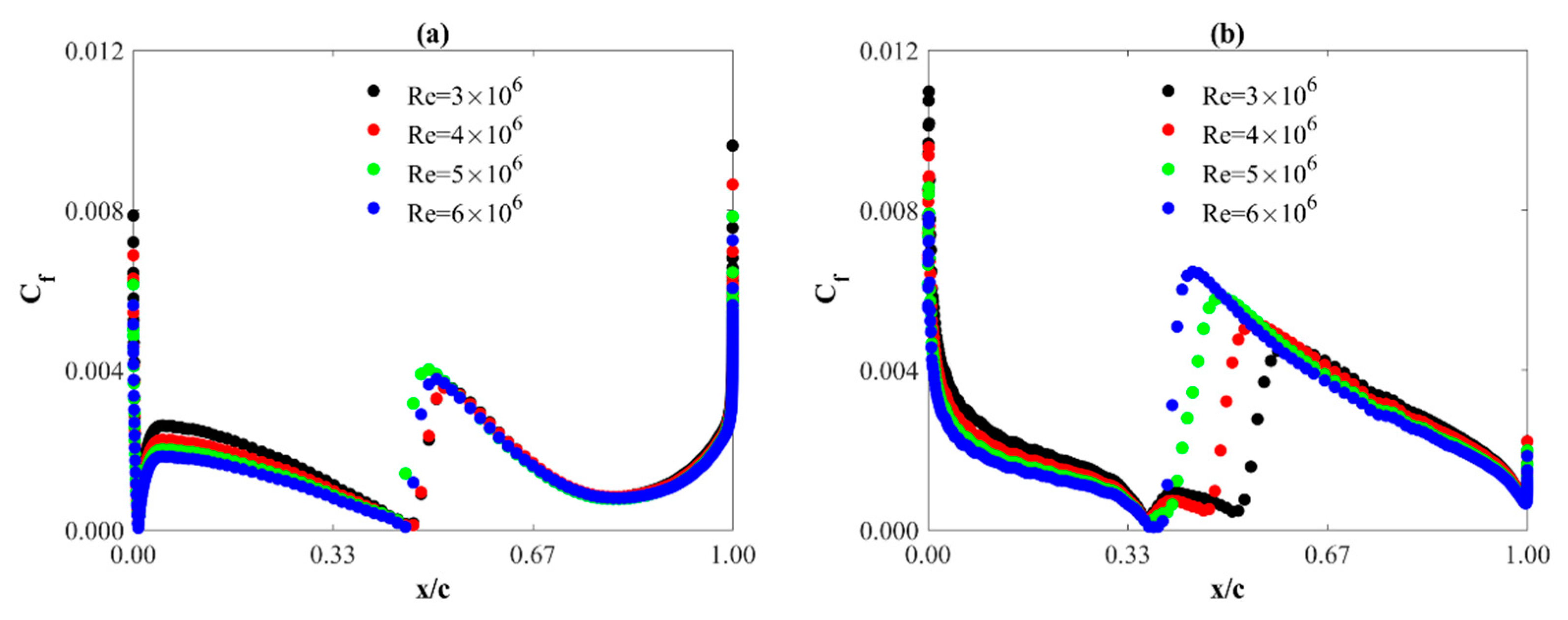
Characteristics of the C f coefficient separately for the pressure and the suction side of the airfoil are shown in Figure 13. Since the nature of the graphs obtained in this work is similar for all angles of attack analyzed here, the figure only illustrates the results for the angle of attack of 4 degrees. The characteristics shown in this figure are given for four Reynolds numbers: 3 × 10 6 , 4 × 10 6 , 5 × 10 6 , and 6 × 10 6 . Contrary to the static pressure coefficients (Figure 9), the skin friction coefficient distributions significantly depend on the Reynolds number. However, it should be emphasized that the influence of the Reynolds number is mainly visible on the suction side of the airfoil (Figure 13b). As the Reynolds number increases, the maximum value of the C f coefficient increases in the middle part of the airfoil, where the laminar-turbulent transition occurs. Moreover, as the Reynolds number increases, the jump in C f shifts to the leading edge. For the suction side of the airfoil and for the Reynolds number of 6 × 10 6 , the maximum value of the skin friction coefficient C f m a x increased by 40.8% compared to the C f m a x for R e = 3 × 10 6 . At the same time, the maximum value of the C f coefficient for R e = 3 × 10 6 was located at x / c = 0.60 whereas for the R e = 6 × 10 6 , the C f m a x has shifted towards the leading edge to the value x / c = 0.44 . For a Reynolds number of 3 × 10 6 , the maximum value of the C f coefficient for the suction side of the airfoil is 28.1% larger compared to the C f m a x for the pressure side. However, for the Reynolds number of 6 × 10 6 , this value increases to 71.1%. The increase of the C f m a x with the increase of the Reynolds number is linear on the suction surface of the airfoil.
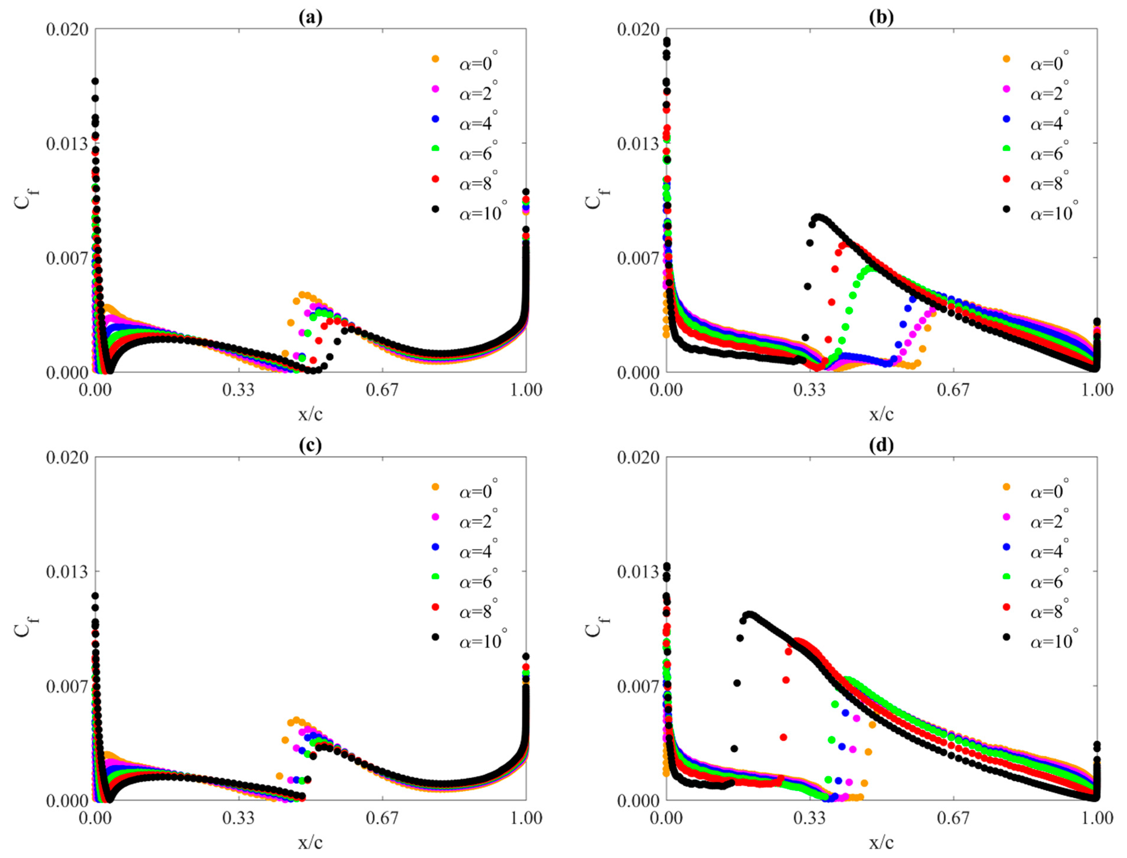
The effect of the Reynolds number on the distribution of the skin friction coefficient is discussed above. The second important factor influencing this physical quantity is the angle of attack. Figure 14 discusses the C f distributions for two Reynolds numbers and for six angles of attack ranging from 0 to 10 degrees. Additionally, as already stated above, the C f distributions are different on the suction and pressure side of the airfoil, therefore Figure 14 compares the C f distributions for both sides of the airfoil separately.
As mentioned above and shown in Figure 13, the Reynolds number effect is more visible on the suction side of the airfoil. As shown in Figure 14, this conclusion applies to all Reynolds numbers analyzed in this work. Moreover, as documented in Figure 14, the effect of the angle of attack is also larger on the suction side of the airfoil as compared to the pressure side. The C f coefficient for both sides of the airfoil differs both in its maximum value and in its x / c location. As the angle of attack increases on the suction side of the airfoil, the maximum value of the C f coefficient moves towards the leading edge and towards the trailing edge on the pressure side of the airfoil. Moreover, as the angle of attack increases, the C f m a x increases on the suction side of the airfoil and decreases on the pressure side. For a Reynolds number equal to 3 × 10 6 , with an angle of attack increment equal to 10 degrees ( Δ α = 10 ° ), the absolute value of the Δ x / c increment corresponding to the C f m a x is 0.3126 on the suction surface and 0.1148 on the pressure surface. For a Reynolds number of 6 × 10 6 , the same values are respectively 0.3166 for the suction side and 0.0647 for the pressure side. It can be concluded from this analysis that with the increase of the Reynolds number, the value of the Δ x / c on the suction side is almost constant and it has been shortened by half on the pressure side. For all the angles of attack analyzed in this paper, on the pressure side of the airfoil, the decrease in the maximum value of the C f coefficient with the increase in the angle of attack is approximately linear whereas on the suction side of the airfoil, the increase in the maximum value of the C f coefficient with the increase in the angle of attack is an exponential function.
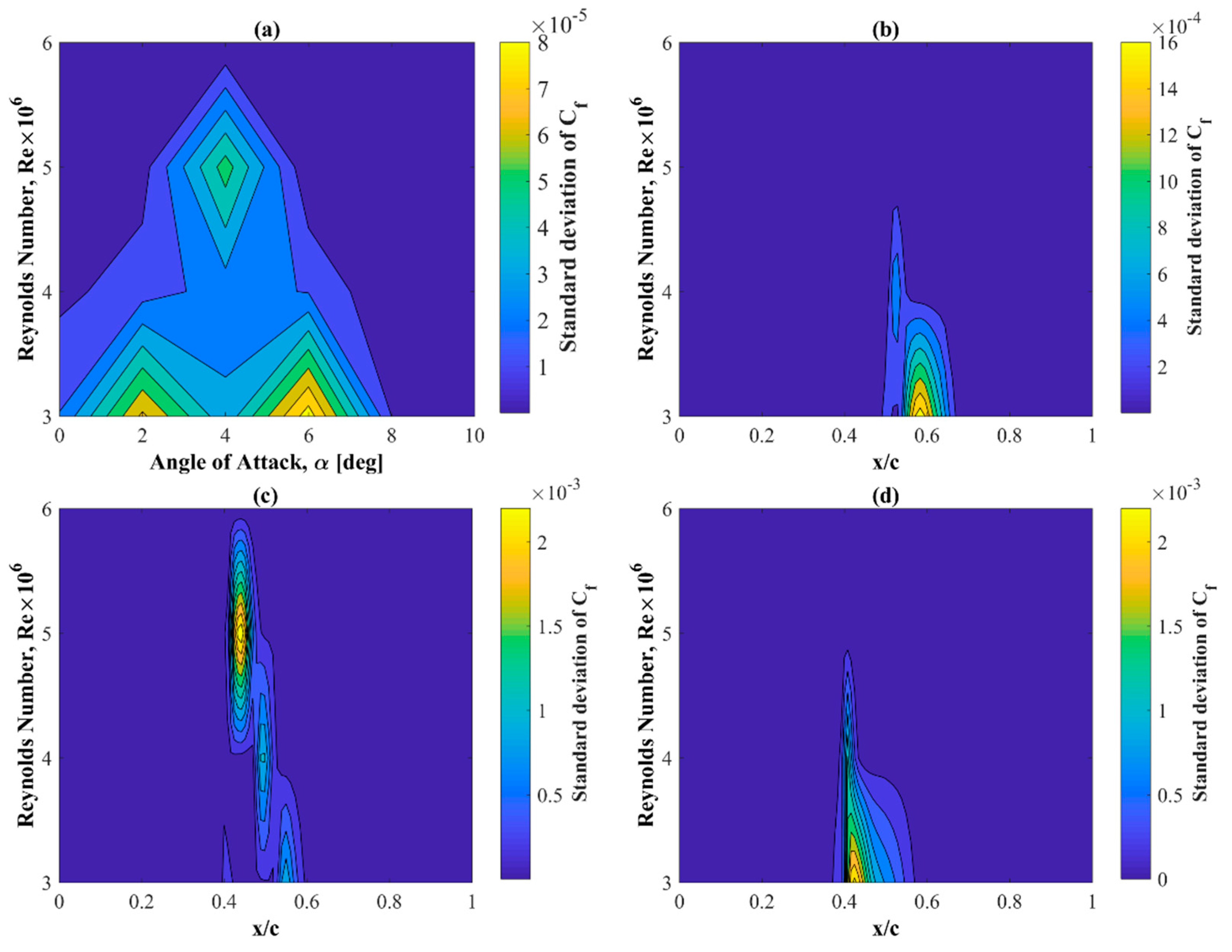
As in the case of static pressure distributions (Section 4.2 and Figure 11), this work also examined the deviations of the instantaneous values of the skin friction coefficient from the average value (Figure 15). This paper also uses the standard deviation formula (Equation (8)) to evaluate this deviation. As with the static pressure distributions, the values of the standard deviation for the suction side of the airfoil are much larger than for the pressure side (please see Section 4.2). In the case of the C f coefficient, the STD results for the suction side of the airfoil are on average 11 times higher compared to the pressure side. The values of the standard deviation of the skin friction coefficient turned out to be small of the higher order and almost 99 times lower compared to the values of the standard deviation calculated for the static pressure coefficients.

4.4. Variation of Transition Location with the Angle of Attack

The location of the transition is a very important engineering issue in modern fluid mechanics; however, it is not easy to determine. For the XFOIL code, this position is one of the simulation results. In the case of CFD analyzes, this location can be found on the basis of intermittency, γ . In our CFD studies, however, this position was estimated from the distribution of the skin friction coefficient C f , discussed in the previous subsection. In order to estimate the transition location X t r the point where the skin friction increases sharply, e.g., as shown in Figure 14, was chosen. This is more consistent with the way the transition is determined experimentally where the intermittency is not known, e.g., using hot film sensors to directly measure the skin friction or a take thermal image of the airfoil surface and see when the heat flux often changes very sharply. Therefore, in this work, to determine this value, a criterion was used, which was established on the basis of the C f results obtained from the XFOIL approach. It was found that the position of X t r corresponds to an increase of the C f coefficient by 80% compared to the minimum value.
Figure 16 compares the location X t r of the laminar-turbulent transition predicted by the two analytical approaches and with the experiment. In this work, the analytical approaches used for the comparison are the Transition SST turbulence model implemented in the ANSYS Fluent CFD code and the XFOIL code. All simulations were carried out for the range of angles of attack in the range from 0 to 10 degrees. The authors of this work had only experimental data for the suction side of the airfoil.
In Figure 16, it can be seen that two distinct areas are visible on the suction side of the airfoil. The X t r ( α ) curves shown in this figure have two derivatives: in the range of angles of attack from 0 to 6 degrees for the first area, and in the range of angles of about 6 to 10 degrees for the second area. On the other hand, the relationship of the X t r -coordinate for the pressure side of the profile is almost linear over the entire range of angles of attack taken into account in this paper.

5. Conclusions

The main purpose of the present study is to validate the unsteady Reynolds averaged Navier-Stokes (URANS) approach together with the four-equation transition SST turbulence model with experimental data from a wind tunnel. The main computational fluid dynamics (CFD) code used in this work was ANSYS Fluent v 19.0. For comparison, two more CFD codes with the Transition SST model were used: FLOWer and STAR-CCM +. The obtained airfoil characteristics were also compared with the results of fully turbulent models published in other papers. The XFOIL approach was also used in this work for comparison. Based on the obtained results, it was determined that:
  • The aerodynamic characteristics obtained by means of classical turbulence models prove the important role of transition phenomena in the boundary layer.
  • For the studied range of Reynolds numbers, the static pressure distributions do not significantly depend on the Reynolds number.
  • The angle of attack has a much more significant influence on the pressure around the airfoil.
  • Contrary to static pressure distributions, the skin friction coefficient distributions depend on both the angle of attack and the Reynolds number. However, the Reynolds number effect is mainly seen on the suction side of the airfoil. An increase in the Reynolds number causes an increase in the value of this coefficient on the suction edge and its shift towards the leading edge.
  • For all the angles of attack analyzed in this study, on the pressure side of the profile, the decrease in the maximum value of the skin friction coefficient with the increase in the angle of attack is almost linear.
  • On the suction side of the profile, the increase in the maximum value of the skin friction coefficient with the increase in the angle of attack is an exponential function.
  • As with static pressure, the angle of attack has a larger effect on the distribution of the skin friction coefficient than the Reynolds number, but mainly for the suction side of the airfoil.
  • With the increase of the angle of attack, the maximum value of the skin friction coefficient increases on the suction side and decreases on the pressure side.
  • For the angle of attack range investigated, the maximum values of the skin friction coefficient are larger on the suction side of the airfoil compared to the pressure side. As the Reynolds number increases, the difference is larger.
  • The deviations of the instantaneous pressure values from the average value are minimal.
  • The maximum values of the standard deviation of the static pressure coefficients are concentrated around the areas of the laminar-turbulent transition.
  • The deviations of the instantaneous values of the skin friction coefficients from the averaged values are almost constant in time and close to zero.

Author Contributions

Conceptualization, K.R.; methodology, J.M., K.R., G.B. and M.O.L.H.; software, J.M., K.R., G.B. and M.O.L.H.; validation K.R. and J.M.; numerical analysis, J.M., K.R., G.B. and M.O.L.H.; writing—original draft preparation, K.R.; writing—review and editing, J.M., K.R., G.B. and M.O.L.H.; visualization, J.M. and K.R., supervision, G.B. and M.O.L.H. All authors have read and agreed to the published version of the manuscript.

Funding

This research was carried out with the support of the Interdisciplinary Centre for Mathematical and Computational Modelling ICM) University of Warsaw under computational allocation no GB83-33.

Institutional Review Board Statement

Not applicable.

Informed Consent Statement

Not applicable.

Data Availability Statement

Data sharing not applicable.

Conflicts of Interest

The authors declare no conflict of interest.

Nomenclature

Symbol
cchord length
α angle of attack
L lift force
D drag force
C ¯ L mean lift coefficient
C ¯ D mean drag coefficient
Δ t time step size
V undisturbed flow velocity
Klift-to-drag ratio
P static pressure
P r e f reference static pressure
q r e f reference dynamic pressure
ρ free stream density
V free stream velocity
S T D standard deviation
C f skin friction coefficient
C f m a x maximum skin friction coefficient
C P static pressure coefficient
X t r location of the laminar-turbulent transition

References

  1. Kaldellis, J.K.; Apostolou, D.; Kapsali, M.; Kondili, E. Environmental and social footprint of offshore wind energy. Comparison with onshore counterpart. Renew. Energy 2016, 92, 543–556. [Google Scholar] [CrossRef]
  2. Loukogeorgaki, E.; Vagiona, D.G.; Vasileiou, M. Site Selection of Hybrid Offshore Wind and Wave Energy Systems in Greece Incorporating Environmental Impact Assessment. Energies 2018, 11, 2095. [Google Scholar] [CrossRef]
  3. Tescione, G.; Sim~ao Ferreira, C.J.; van Bussel, G.J.W. Analysis of a free vortex wake model for the study of the rotor and near wake flow of a vertical axis wind turbine. Renew. Energy 2016, 87, 552–563. [Google Scholar] [CrossRef]
  4. Wind in Our Sails. The Coming of Europe’s Offshore Wind Energy Industry; Technical Report; European Wind Energy Association (EWEA), 2011. Available online: https://tethys.pnnl.gov/publications/wind-our-sails-coming-europes-offshore-wind-energy-industry (accessed on 1 December 2021).
  5. Hu, Y.; Yang, J.; Baniotopoulos, C. Study of the Bearing Capacity of Stiffened Tall Offshore Wind Turbine Towers during the Erection Phase. Energies 2020, 13, 5102. [Google Scholar] [CrossRef]
  6. Castro-Santos, L.; Filgueira-Vizoso, A.; Álvarez-Feal, C.; Carral, L. Influence of Size on the Economic Feasibility of Floating Offshore Wind Farms. Sustainability 2018, 10, 4484. [Google Scholar] [CrossRef] [Green Version]
  7. Yang, H.; Shen, W.Z.; Xu, H.; Hong, Z.; Liu, C. Prediction of the wind turbine performance by using BEM with airfoil data extracted from CFD. Renew. Energy 2014, 70, 107–115. [Google Scholar] [CrossRef]
  8. Zidane, I.F.; Swadener, G.; Ma, X.; Shehadeh, M.F.; Salem, M.H.; Saqr, K.M. Performance of a Wind Turbine Blade in Sandstorms Using a CFD-BEM Based Neural Network. J. Renew. Sustain. Energy 2020, 12, 053310. [Google Scholar] [CrossRef]
  9. Rogowski, K.; Królak, G.; Bangga, G. Numerical Study on the Aerodynamic Characteristics of the NACA 0018 Airfoil at Low Reynolds Number for Darrieus Wind Turbines Using the Transition SST Model. Processes 2021, 9, 477. [Google Scholar] [CrossRef]
  10. Monteiro, J.P.; Silvestre, M.R.; Piggott, H.; Andre, J.C. Wind tunnel testing of a horizontal axis wind turbine rotor and comparison with simulations from two blade element momentum codes. J. Wind Eng. Ind. Aerod. 2013, 123, 99–106. [Google Scholar] [CrossRef]
  11. Bai, C.-J.; Wang, W.-C. Review of computational and experimental approaches to analysis of aerodynamic performance in horizontal-axis wind turbines (HAWTs). Renew. Sustain. Energy Rev. 2016, 63, 506–519. [Google Scholar] [CrossRef]
  12. Rogowski, K.; Maroński, R.; Hansen, M.O.L. Steady and unsteady analysis of NACA 0018 airfoil in vertical-axis wind turbine. J. Theor. Appl. Mech. 2018, 51, 203–212. [Google Scholar] [CrossRef] [Green Version]
  13. Timmer, W.A. Two-Dimensional Low-Reynolds Number Wind Tunnel Results for Airfoil NACA 0018. Wind. Eng. 2008, 32, 525–537. [Google Scholar] [CrossRef] [Green Version]
  14. Sanei, M.; Razaghi, R. Numerical investigation of three turbulence simulation models for S809 wind turbine airfoil. Proc. Inst. Mech. Eng. Part A J. Power Energy 2018, 232, 1037–1048. [Google Scholar] [CrossRef]
  15. Rogowski, K.; Hansen, M.O.L. RANS Simulations of Flow Past an DU-91-W2-250 Airfoil at High Reynolds Number. In Proceedings of the 10th Conference on Interdisciplinary Problems in Environmental Protection and Engineering EKO-DOK, Polanica-Zdrój, Poland, 16–18 April 2018. [Google Scholar] [CrossRef]
  16. Bak, C.; Zahle, F.; Bitsche, R.; Kim, T.; Yde, A.; Henriksen, L.C.; Natarajan, A.; Hansen, M.H. Description of the DTU 10 MW Reference Wind Turbine. DTU Wind Energy Report-I-0092. 2013. Available online: https://orbit.dtu.dk/en/publications/the-dtu-10-mw-reference-wind-turbine (accessed on 1 December 2021).
  17. Drela, M. XFOIL: An Analysis and Design System for Low Reynolds Number Airfoils; Low Reynolds Number Aerodynamics. Lecture Notes in Engineering; Mueller, T.J., Ed.; Springer: Berlin/Heidelberg, Germany, 1989; Volume 54. [Google Scholar] [CrossRef]
  18. Fontecha, R.; Kemper, F.; Feldmann, M. On the Determination of the Aerodynamic Damping of Wind Turbines Using the Forced Oscillations Method in Wind Tunnel Experiments. Energies 2019, 12, 2452. [Google Scholar] [CrossRef] [Green Version]
  19. Rogowski, K.; Hansen, M.O.L.; Bangga, G. Performance Analysis of a H-Darrieus Wind Turbine for a Series of 4-Digit NACA Airfoils. Energies 2020, 13, 3196. [Google Scholar] [CrossRef]
  20. Lichota, P. Multi-Axis Inputs for Identification of a Reconfigurable Fixed-Wing UAV. Aerospace 2020, 7, 113. [Google Scholar] [CrossRef]
  21. Lichota, P.; Noreña, D.A. A Priori Model Inclusion in the Multisine Maneuver Design. In Proceedings of the 17th International Carpathian Control Conference, High Tatras, Slovakia, 29 May–1 June 2016; pp. 440–445. [Google Scholar] [CrossRef]
  22. Wolfe, W.P.; Ochs, S.S. CFD Calculations of S809 Aerodynamic Characteristics. In Proceedings of the 35th Aerospace Sciences Meeting and Exhibit, AIAA, Reno, NV, USA, 6–9 January 1997. [Google Scholar]
  23. Rogowski, K.; Hansen, M.O.L.; Maroński, R.; Lichota, P. Scale Adaptive Simulation Model for the Darrieus Wind Turbine. J. Phys. Conf. Ser. 2016, 753, 022050. [Google Scholar] [CrossRef]
  24. Zhong, W.; Tang, H.; Wang, T.; Zhu, C. Accurate RANS Simulation of Wind Turbine Stall by Turbulence Coefficient Calibration. Appl. Sci. 2018, 8, 1444. [Google Scholar] [CrossRef] [Green Version]
  25. Mo, J.-o.; Rho, B.-s. Characteristics and Effects of Laminar Separation Bubbles on NREL S809 Airfoil Using the γ—R e θ Transition Model. Appl. Sci. 2020, 10, 6095. [Google Scholar] [CrossRef]
  26. D’Alessandro, V.; Montelpare, S.; Ricci, R. Assessment of a Spalart–Allmaras Model Coupled with Local Correlation Based Transition Approaches for Wind Turbine Airfoils. Appl. Sci. 2021, 11, 1872. [Google Scholar] [CrossRef]
  27. Kubacki, S.; Simoni, D.; Lengani, D.; Dellacasagrande, M.; Dick, E. Extension of an algebraic intermittency model for better prediction of transition in separated layers under strong free-stream turbulence. Int. J. Heat Fluid Flow 2021, 92, 108860. [Google Scholar] [CrossRef]
  28. Rezaeiha, A.; Montazeri, H.; Blocken, B. Towards accurate CFD simulations of vertical axis wind turbines at different tip speed ratios and solidities: Guidelines for azimuthal increment, domain size and convergence. Energy Convers. Manag. 2018, 156, 301–316. [Google Scholar] [CrossRef]
  29. Schlichting, H. Boundary Layer Theory, 7th ed.; McGraw-Hill: New York, NY, USA, 1979. [Google Scholar]
  30. Morkovin, M.V. On the Many Faces of Transition; Viscous Drag Reduction; Wells, C.S., Ed.; Plenum Press: New York, NY, USA, 1969; pp. 1–31. [Google Scholar]
  31. Mayle, R.E. The role of laminar-turbulent transition in gas turbine engines. J. Turbomach. 1991, 113, 509–537. [Google Scholar] [CrossRef]
  32. Dick, E.; Kubacki, S. Transition Models for Turbomachinery Boundary Layer Flows: A Review. Int. J. Turbomach. Propuls. Power 2017, 2, 4. [Google Scholar] [CrossRef] [Green Version]
  33. Liu, G.; Sun, S.; Liang, K.; Yang, X.; An, D.; Wen, Q.; Ren, X. Simulation Study on the Effect of Flue Gas on Flow Field and Rotor Stress in Gas Turbines. Energies 2021, 14, 6135. [Google Scholar] [CrossRef]
  34. Engelmann, D.; Sinkwitz, M.; di Mare, F.; Koppe, B.; Mailach, R.; Ventosa-Molina, J.; Fröhlich, J.; Schubert, T.; Niehuis, R. Near-Wall Flow in Turbomachinery Cascades—Results of a German Collaborative Project. Int. J. Turbomach. Propuls. Power 2021, 6, 9. [Google Scholar] [CrossRef]
  35. Langtry, R.B. A Correlation-Based Transition Model Using Local Variables for Unstructured Parallelized CFD Codes. Ph.D. Thesis, University of Stuttgart, Stuttgart, Germany, 2006. [Google Scholar] [CrossRef]
  36. Smith, A.M.O.; Gamberoni, N. Transition, Pressure Gradient and Stability Theory; Douglas Aircraft Company, El Segundo Division: Los Angeles, CA, USA, 1956. [Google Scholar]
  37. Van Ingen, J.L. A Suggested Semi-Empirical Method for the Calculation of the Boundary Layer Transition Region; Report VTH-74; Department of Aerospace Engineering, Delft University of Technology: Delft, The Netherlands, 1956. [Google Scholar]
  38. Themistokleous, C.; Markatos, N.-G.; Prospathopoulos, J.; Riziotis, V.; Sieros, G.; Papadakis, G. A High-Lift Optimization Methodology for the Design of Leading and Trailing Edges on Morphing Wings. Appl. Sci. 2021, 11, 2822. [Google Scholar] [CrossRef]
  39. Youngren, H.; Drela, M. Viscous/Inviscid method for preliminary design of transonic cascades. In Proceedings of the 27th Joint Propulsion Conference, Sacramento, CA, USA, 24–26 June 1991. [Google Scholar]
  40. Stock, H.W. eN Transition prediction in three-dimensional boundary layers on inclined prolate spheroids. AIAA J. 2006, 44, 108–118. [Google Scholar] [CrossRef]
  41. Menter, F.R.; Langtry, R.B. Transition Modelling for Turbomachinery Flows. In Low Reynolds Number Aerodynamics and Transition; Genc, M.S., Ed.; InTech: London, UK, 2012; Available online: http://www.intechopen.com/books/low-reynolds-number-aerodynamics-and-transition/transitionmodelling-for-turbomachinery-flows (accessed on 21 October 2021)ISBN 978-953-51-0492-6.
  42. Vlahostergios, Z. Performance Assessment of Reynolds Stress and Eddy Viscosity Models on a Transitional DCA Compressor Blade. Aerospace 2018, 5, 102. [Google Scholar] [CrossRef] [Green Version]
  43. Timmer, W.A.; van Rooij, R.P.J.O.M. Summary of the Delft University Wind Turbine Dedicated Airfoils. J. Sol. Energy Eng. 2003, 125, 488–496. [Google Scholar] [CrossRef]
  44. van Rooij, R.P.J.O.M.; Timmer, W.A. Roughness Sensitivity Considerations for Thick Rotor Blade Airfoils. J. Sol. Energy Eng. 2003, 125, 468–478. [Google Scholar] [CrossRef]
  45. Ahmed, R.M. Blade sections for wind turbine and tidal current turbine applications—Current status and future challenges. Int. J. Energy Res. 2012, 36, 829–844. [Google Scholar] [CrossRef]
  46. Schubel, P.J.; Crossley, R.J. Wind Turbine Blade Design. Energies 2012, 5, 3425–3449. [Google Scholar] [CrossRef] [Green Version]
  47. Baldacchino, D.; Manolesos, M.; Ferreira, C.; Gonzάlez Salcedo, Á.; Aparicio, M.; Chaviaropoulos, T.; Diakakis, K.; Florentie, L.; Garcίa, N.G.; Papadakis, G.; et al. Experimental benchmark and code validation for airfoils equipped with passive vortex generators. J. Phys. Conf. Ser. 2016, 753, 022002. [Google Scholar] [CrossRef]
  48. Velte, C.M.; Hansen, M.O.L.; Meyer, K.E. Evaluation of the Performance of Vortex Generators on the DU 91-W2-250 Profile using Stereoscopic PIV. In Proceedings of the WMSCI 2008: 12th World Multi-Conference on Systemics, Cybernetics and Informatics, Orlando, FL, USA, 29 June–2 July 2008; Volume 2, pp. 263–267. [Google Scholar]
  49. Bak, C.; Gaunaa, M.; Olsen, A.S.; Kruse, E.K. What is the critical height of leading edge roughness for aerodynamics? J. Phys. Conf. Ser. 2016, 753, 022023. [Google Scholar] [CrossRef]
  50. Langel, C.M. A Transport Equation Approach to Modeling the Influence of Surface Roughness on Boundary Layer Transition. Master’s Thesis, University of California, Albuquerque, NM, USA, 2014. [Google Scholar]
  51. Ren, N.; Ou, J. Numerical Simulation of Surface Roughness Effect on Wind Turbine Thick Airfoils. In Proceedings of the 2009 Asia-Pacific Power and Energy Engineering Conference, Wuhan, China, 27–31 March 2009; pp. 1–4. [Google Scholar] [CrossRef]
  52. Langtry, R.B.; Gola, J.; Menter, F.R. Predicting 2D Airfoil and 3D Wind Turbine Rotor Performance using a Transition Model for General CFD Codes. In Proceedings of the 44th AIAA Aerospace Sciences Meeting and Exhibit, Reno, NV, USA, 9–12 January 2006. AIAA 2006-395. [Google Scholar]
  53. Xu, H.; Shen, W.; Zhu, W.; Yang, H.; Liu, C. Aerodynamic Analysis of Trailing Edge Enlarged Wind Turbine Airfoils. J. Phys. Conf. Ser. 2014, 524, 012010. [Google Scholar] [CrossRef] [Green Version]
  54. Bangga, G.; Lutz, T.; Schwarz, E.; Krämer, E. CFD studies on rotational augmentation at the inboard sections of a 10 MW wind turbine rotor. Renew. Sust. Energ. Rev. 2017, 9, 023304. [Google Scholar] [CrossRef]
  55. Zhang, Y.; Sun, Z.; van Zuijlen, A.; van Bussel, G. Numerical simulation of transitional flow on a wind turbine airfoil with RANS-based transition model. J. Turbul. 2017, 18, 879–898. [Google Scholar] [CrossRef] [Green Version]
  56. Bangga, G.; Kusumadewi, T.; Hutomo, G.; Sabila, A.; Syawitri, T.; Setiadi, H.; Faisa, M.; Wiranegara, R.; Hendranata, Y.; Lastomo, D.; et al. Improving a two-equation eddy-viscosity turbulence model to predict the aerodynamic performance of thick wind turbine airfoils. J. Phys. Conf. Ser. 2018, 974, 012019. [Google Scholar] [CrossRef]
  57. Bangga, G.; Lutz, T.; Krämer, E. Active separation control on a very thick wind turbine airfoil—A URANS and DDES perspective. J. Phys. Conf. Ser. 2018, 1037, 022025. [Google Scholar] [CrossRef] [Green Version]
  58. Rogowski, K.; Hansen, M.O.L.; Hansen, R.; Piechna, J.; Lichota, P. Detached Eddy Simulation Model for the DU-91-W2-250 Airfoil. J. Phys. Conf. Ser. 2018, 1037, 022019. [Google Scholar] [CrossRef] [Green Version]
  59. Chillon, S.; Uriarte-Uriarte, A.; Aramendia, I.; Martínez-Filgueira, P.; Fernandez-Gamiz, U.; Ibarra-Udaeta, I. jBAY Modeling of Vane-Type Vortex Generators and Study on Airfoil Aerodynamic Performance. Energies 2020, 13, 2423. [Google Scholar] [CrossRef]
  60. Campobasso, M.S.; Castorrini, A.; Cappugi, L.; Bonfiglioli, A. Experimentally validated three-dimensional computational aerodynamics of wind turbine blade sections featuring leading edge erosion cavities. Wind. Energy 2021, 1–22. [Google Scholar] [CrossRef]
  61. Cao, N. Effects of Turbulence Intensity and Integral Length Scale on an Asymmetric Airfoil at Low Reynolds Numbers. Master’s Thesis, University of Windsor, Windsor, ON, USA, 2010. [Google Scholar]
  62. Butler, R.J.; Byerley, A.R.; VanTreuren, K.; Baughn, J.W. The effect of turbulence intensity and length scale on low-pressure turbine blade aerodynamics. Int. J. Heat Fluid Flow 2001, 22, 123–133. [Google Scholar] [CrossRef]
  63. Menter, F.R.; Smirnov, P.E.; Liu, T.A. One-Equation Local Correlation-Based Transition Model. Flow Turbul. Combust. 2015, 95, 583–619. [Google Scholar] [CrossRef]
  64. Wang, H.; Ding, J.; Ma, G.; Li, S. Aerodynamic simulation of wind turbine blade airfoil with different turbulence models. J. Vibroeng. 2014, 16, 2474–2483. [Google Scholar]
  65. Gupta, M.K.; Subbarao, P.M.V. Development of a semi-analytical model to select a suitable airfoil section for blades of horizontal axis hydrokinetic turbine. In Proceedings of the 6th International Conference on Energy and Environment Research, ICEER 2019, Aveiro, Portugal, 22–25 July 2019; Energy Reports 6, 2020. University of Aveiro: Aveiro, Portugal, 2019; pp. 32–37. [Google Scholar] [CrossRef]
  66. Kruse, E.K.; Sorensen, N.N.; Bak, C. A twodimensional quantitative parametric investigation of simplified surface imperfections on the aerodynamic characteristics of a NACA 633 418 airfoil. Wind. Energy 2021, 24, 310–322. [Google Scholar] [CrossRef]
  67. ANSYS Fluent Theory Guide Version 19. Available online: https://www.ansys.com/products/fluids/ansys-fluent (accessed on 1 December 2021).
  68. Thomas, J.L.; Salas, M.D. Far-field boundary conditions for transonic lifting solutions to the Euler equations. AIAA J. 1986, 24, 1074–1080. [Google Scholar] [CrossRef]
  69. Wang, H.; Zhang, B.; Qiu, Q.; Xu, X. Flow control on the NREL S809 wind turbine airfoil using vortex generators. Energy 2017, 118, 1210–1221. [Google Scholar] [CrossRef]
  70. Lu, S.; Liu, J.; Hekkenberg, R. Mesh Properties for RANS Simulations of Airfoil-Shaped Profiles: A Case Study of Rudder Hydrodynamics. J. Mar. Sci. Eng. 2021, 9, 1062. [Google Scholar] [CrossRef]
  71. Menter, F.R.; Langtry, R.; Völker, S. Transition Modelling for General Purpose CFD Codes. Flow Turbul. Combust. 2006, 77, 277–303. [Google Scholar] [CrossRef]
  72. Şahin, I.; Acir, A. Numerical and Experimental Investigations of Lift and Drag Performances of NACA 0015 Wind Turbine Airfoil. Int. J. Mater. Mech. Manuf. 2015, 3, 22–25. [Google Scholar] [CrossRef] [Green Version]
  73. Xiao, S.; Chen, Z. Investigation of Flow over the Airfoil NACA 0010-35 with Various Angle of Attack. In Proceedings of the MATEC Web of Conferences 179, 03020, Wuhan, China, 10–13 May 2018. [Google Scholar] [CrossRef]
  74. Ockfen, A.E.; Matveev, K.I. Aerodynamic characteristics of NACA 4412 airfoil section with flap in extreme ground effect. Int. J. Nav. Archit 2009, 1, 1–12. [Google Scholar] [CrossRef] [Green Version]
  75. Aftab, S.M.A.; Mohd Rafie, A.S.; Razak, N.A.; Ahmad, K.A. Turbulence Model Selection for Low Reynolds Number Flows. PLoS ONE 2016, 11, e0153755. [Google Scholar] [CrossRef] [PubMed] [Green Version]
  76. Abdul Hamid, M.; Toufique Hasan, A.B.M.; Alimuzzaman, S.M.; Matsuo, S.; Setoguchi, T. Compressible flow characteristics around a biconvex arc airfoil in a channel. Propuls. Power Res. 2014, 3, 29–40. [Google Scholar] [CrossRef] [Green Version]
  77. Jansson, L.; Lövmark, J. An Investigation of the Dynamic Characteristics of a Tilting Disc Check Valve Using CFD Analyses. Master’s Thesis, Chalmers University of Technology, Göteborg, Sweden, 2013. [Google Scholar]
  78. Menter, F.R.; Langtry, R.B.; Likki, S.R.; Suzen, Y.B.; Huang, P.G.; Völker, S. A correlationbased transition model using local variables—part I: Model formulation. J. Turbomach. 2006, 128, 413–422. [Google Scholar] [CrossRef]
  79. Langtry, R.B.; Menter, F.R.; Likki, S.R.; Suzen, Y.B.; Huang, P.G.; Völker, S. A correlation based transition model using local variables—part II: Test cases and industrial applications. J. Turbomach. 2006, 128, 423–434. [Google Scholar] [CrossRef]
  80. Wang, S.; Ingham, D.B.; Ma, L.; Pourkashanian, M.; Tao, Z. Turbulence modeling of deep dynamic stall at relatively low Reynolds number. J. Fluids Struct. 2012, 33, 191–209. [Google Scholar] [CrossRef]
  81. Morgado, J.; Vizinho, R.; Silvestre, M.A.R.; Páscoa, J.C. XFOIL vs. CFD performance predictions for high lift low Reynoldsnumber airfoils. Aerosp. Sci. Technol. 2016, 52, 207–214. [Google Scholar] [CrossRef]
  82. Drela, M.; Giles, M. Viscous-Inviscid Analysis of Transonic and Low Reynolds Number Airfoils. AIAA J. 1987, 25, 1347–1355. [Google Scholar] [CrossRef]
  83. Nieroba, W. Application of the k-ε Turbulence Model in the Analysis of the Flow over DU 91-W2-250 Airfoil. Bachelor’s Thesis, Warsaw University of Technology, Faculty of Power and Aeronautical Engineering, Warsaw, Poland, 2019. [Google Scholar]
  84. Królak, G. k-ω Turbulence Model for the DU 91-W2-250 Airfoil at High Reynolds Number. Bachelor’s Thesis, Warsaw University of Technology, Faculty of Power and Aeronautical Engineering, Warsaw, Poland, 2019. [Google Scholar]
  85. Munson, B.R.; Young, D.F.; Okiishi, T.H. Introduction to Fluid Mechanics, 5th ed.; John Wiley & Sons: Hoboken, NJ, USA, 2005. [Google Scholar]
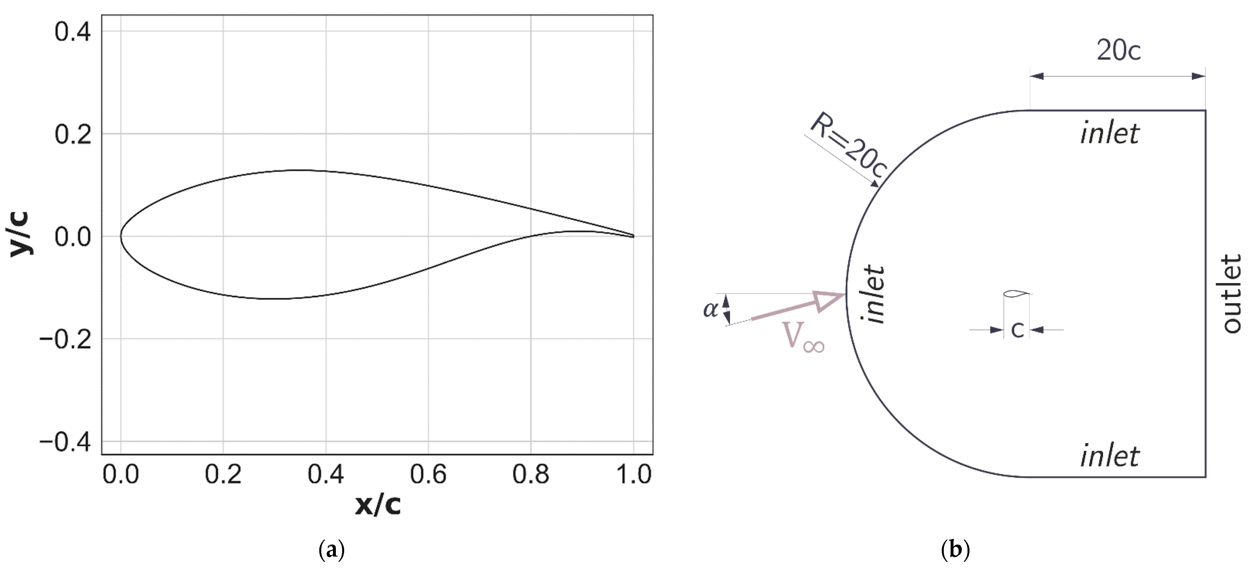
Figure 1. Numerical model: (a) DU-91-W2-250 airfoil; (b) computational domain and boundary conditions.
Energies 14 08224 g001
Figure 2. Mesh: (a) The mesh in the entire computing domain; (b) The distribution of the mesh around the airfoil.
Energies 14 08224 g002
Figure 3. The averaged aerodynamic force coefficients and their standard deviation at the angle of attack of 4°: (a) lift coefficient; (b) drag coefficient.
Energies 14 08224 g003
Figure 4. Mesh: (a) FLOWer; (b) STAR-CCM +.
Energies 14 08224 g004
Figure 5. DU-91-W2-250 airfoil performance for two Reynolds numbers of 3 × 10 6 and 6 × 10 6 .
Energies 14 08224 g005
Figure 6. The drag and lift coefficients as a function of the Reynolds number for six angles of attack: (a,b) drag coefficients; (c,d) lift coefficients; (e,f) torque coefficients. The results are given only for URANS with the Transition SST turbulence model.
Energies 14 08224 g006
Figure 7. Static pressure distributions calculated for different numerical approaches. The results are presented for one angle of attack equal to 4 degrees.
Energies 14 08224 g007
Figure 8. Static pressure distributions calculated for different angles of attack and for different Reynolds numbers.
Energies 14 08224 g008
Figure 9. Effect of the Reynolds number on static pressure coefficient characteristics: (a) airfoil shape; (b) distribution of the static pressure coefficients on the pressure side of the airfoil; (c,d) details of the static pressure distributions on the pressure side of the airfoil—the details are marked in these figures with the appropriate colors.
Energies 14 08224 g009
Figure 10. Static pressure coefficient for Reynolds number of 6 × 10 6 . The influence of the angle of attack.
Energies 14 08224 g010
Figure 11. Standard deviation of the static pressure coefficient for the suction side of the airfoil and for the angle of attack of 4 degrees: (a) as a function of the angle of attack and Reynolds number; (b) as a function of x/c and Reynolds number.
Energies 14 08224 g011
Figure 12. Skin friction coefficient at the angle of attack of 4° for two Reynolds number of 3 × 10 6 (a) and 6 × 10 6 (b). The results are given for three numerical approaches: ANSYS Fluent code together with the URANS method; the k-ε RNG turbulence model; the XFOIL code.
Energies 14 08224 g012
Figure 13. Skin friction coefficient at the angle of attack of 4°—Reynolds number effect for (a) the pressure side of the airfoil and (b) the suction side of the airfoil. These results are given for URANS with the Transition SST model.
Energies 14 08224 g013
Figure 14. Skin friction coefficient—the effect of the angle of attack for (a,b) R e = 3 × 10 6 and (c,d) R e = 6 × 10 6 . Moreover, C f for the pressure side of the airfoil are given in (a,c), whereas for the suction side of the airfoil are given in (b,d). These results are given for URANS with the Transition SST model.
Energies 14 08224 g014
Figure 15. Standard deviation of the skin friction coefficient for the suction side of the airfoil—the effect of the angle of attack and the Reynolds number (a); the effect of the Reynolds number and x/c for: α = 2 ° (b); α = 4 ° (c); and α = 6 ° (d).
Energies 14 08224 g015
Figure 16. Variation of transition location with the angle of attack for two Reynolds numbers. For the suction side of the airfoil: validation of the Transition SST turbulence model and the XFOIL code using the experimental data; for the pressure side: comparison of the results obtained from CFD and XFOIL simulations.
Energies 14 08224 g016
Table 1. Mesh convergence study. The drag coefficient for a different number of nodes on the airfoil surface for the Reynolds number of 4 × 10 6 .
Test Case (No. of Nodes on Airfoil Surface) Drag   Coefficient ,   C D Percentage Difference of Drag Coefficient to Case 1
Case 2 (N/4 = 155)0.00917319.77%
Case 3 (N/2 = 310)0.0083268.71%
Case 1 (N = 620)0.0076590.00%
Case 4 (2N = 1240)0.007459−2.60%
Table 2. The derivative of the lift-to-drag ratio d K / d α for the range of angles of attack from 0° to 4° and for different aerodynamic methods.
Aerodynamic Method d K / d α   ( R e   =   3 × 10 3 ) Relative   Error   ( R e   =   3 × 10 3 ) d K / d α   ( R e   =   6 × 10 3 ) Relative   Error   ( R e   =   6 × 10 3 )
Experiment819.740.00978.810.00
URANS with the Transition SST688.3916.02748.2223.56
RANS with the Transition SST822.900.39789.6819.32
k-ω SST439.0846.44470.9051.89
k-ε414.3949.45471.1151.87
RNG k-ε420.9848.64451.0653.92
STAR-CCM +660.3619.44735.7529.65
FLOWer665.1118.86771.9725.23
XFOIL917.1611.881088.3311.19
Publisher’s Note: MDPI stays neutral with regard to jurisdictional claims in published maps and institutional affiliations.