
Surface Roughness Effects on Flows Past Two Circular Cylinders in Tandem Arrangement at Co-Shedding Regime


Abstract
:1. Introduction
2. The Lagrangian Vortex Method with Model of Surface Roughness Effects
- (i)
- simultaneous solution of the linear systems of algebraic equations to generate source densities and vortex blob strengths (the model of roughness effects can be activated);
- (ii)
- velocity vector calculation at every vortex blob;
- (iii)
- static pressure evaluation on pivotal points followed by drag and lift coefficients computation for two bodies;
- (iv)
- solution of the vortex blobs advection;
- (v)
- solution of the vorticity diffusion including turbulence modeling using LES theory;
- (vi)
- reflection of stray vortex blobs from each body profile interior;
- (vii)
- velocity vector calculation at every pivotal point for new generation of source densities and vortex blobs strength (this step restores the boundary conditions on every pivotal point); and
- (viii)
- advance by ∆t.
3. Results and Discussion
3.1. Simulation Setup
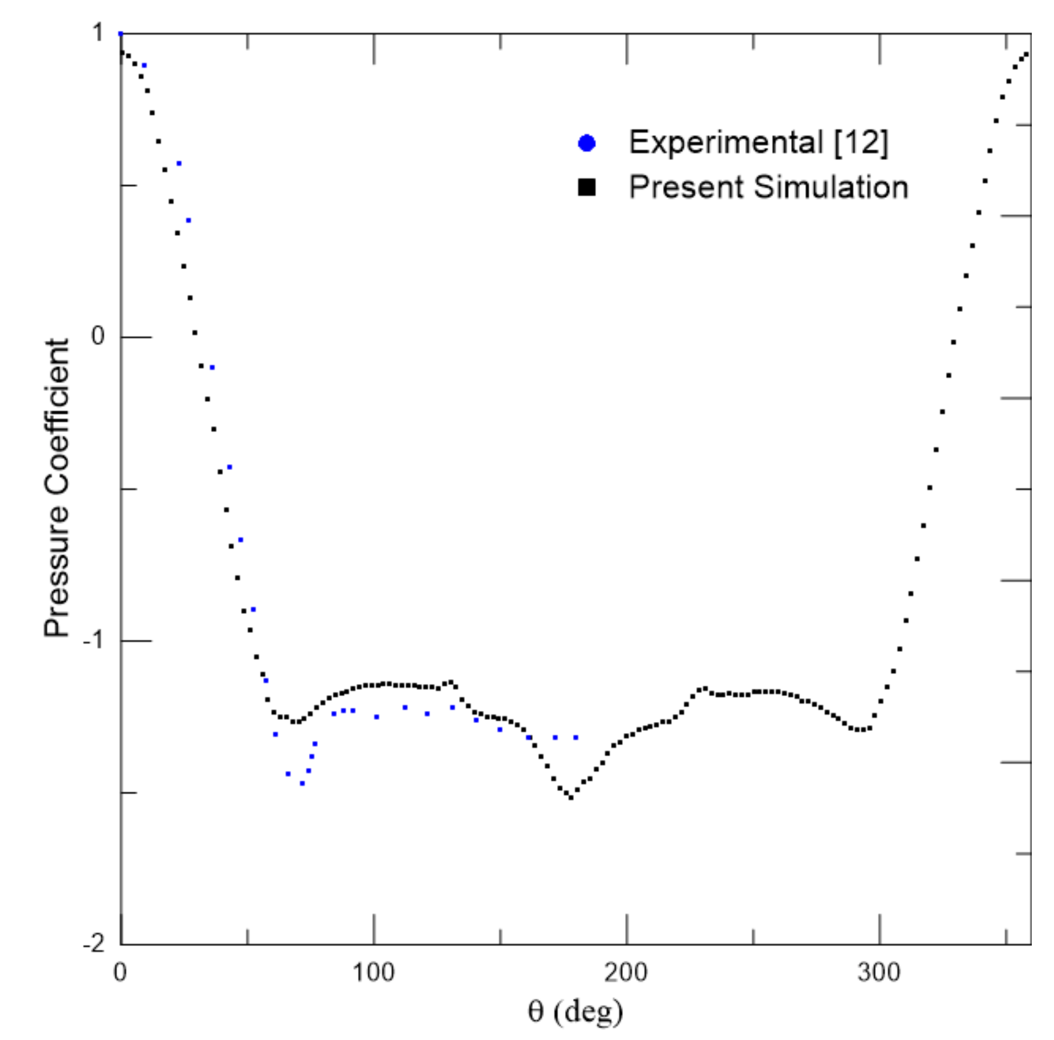
3.2. Smoothed Upstream Circular Cylinder without the Presence of the Downstream Circular Cylinder
3.3. Upstream Circular Cylinder with the Presence of the Downstream Circular Cylinder
4. Conclusions
- (i)
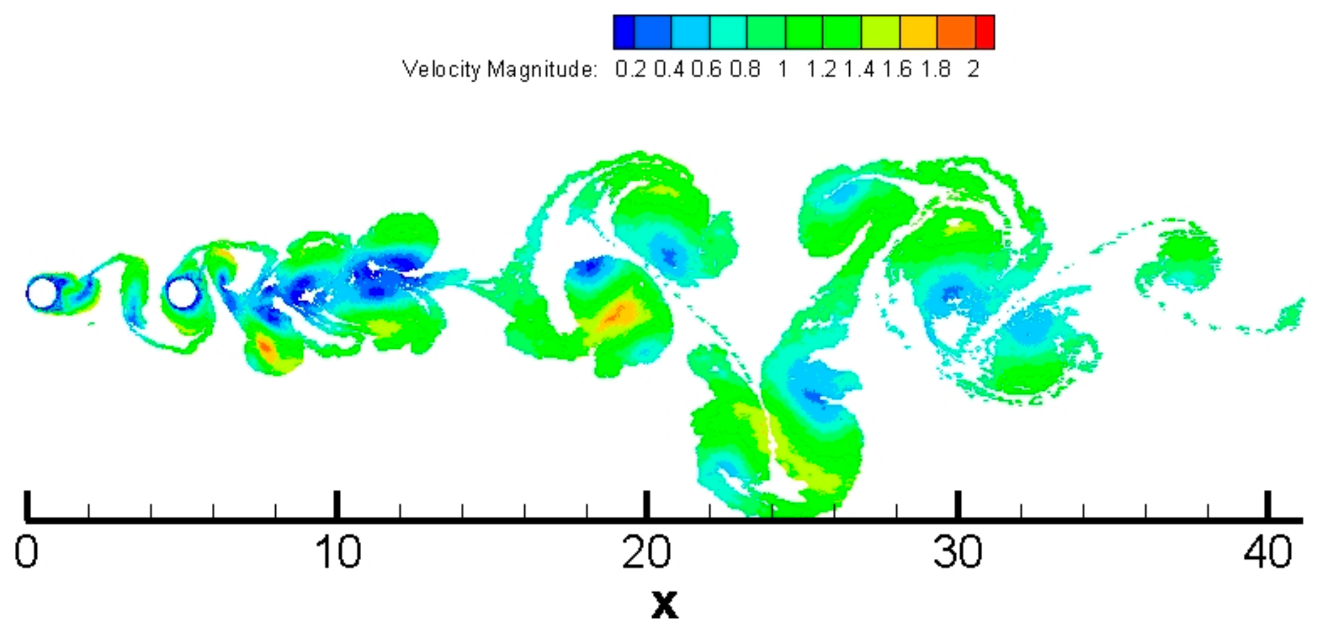
- The relative roughness height of ε/D = 0.001 reduces the Strouhal number of the upstream cylinder about 6.25% when it simulate roughness effects. The mentioned reduction also occurs for the downstream cylinder without or with simulation of surface roughness effects (Table 3). That flow pattern ratifies the expected physics, where the vortical structures from upstream cylinder travel impinge on the downstream cylinder and also govern the vortex-forming regime from the downstream cylinder, as illustrated in Figure 13.
- (ii)
- For ε/D = 0.001, the higher drag reduction on upstream cylinder surface (around of 16.42%) is identified when both the cylinders simulate surface roughness effects. That flow pattern increases the drag force on downstream cylinder about 3.33% (Table 3).
- (iii)
- For ε/D = 0.001, the higher drag reduction on downstream cylinder surface (around of 9.97%) manifests for downstream cylinder simulating roughness effects and smoothed upstream cylinder (ε/D = 0.000). That flow pattern increases the drag force on upstream cylinder around of 2.27% (Table 3).
- (iv)
- Still, for ε/D = 0.001, interestingly, the drag force on downstream cylinder increases about 31.71% when only the upstream cylinder simulates roughness effects. That flow pattern reduces the drag force acting on upstream cylinder by around 14.32% (Table 3).
- (v)
- On the other hand, the relative roughness height of ε/D = 0.007 only reduces the Strouhal number about 6.25% when both cylinders simulate roughness effects (Table 4). That flow pattern indicates that counter-rotating vortical structures from upstream cylinder also travel, impinging on the downstream cylinder and governing the vortex-forming regime from the latter cylinder. As illustration, Figure 14 shows that the higher relative roughness height, simultaneously simulated for both cylinders, provides the most representative wake destructive behavior behind two bodies. A drag reduction on upstream cylinder surface around of 5.04% and about 14.36% on downstream cylinder surface are also identified when both the cylinders include model of surface roughness effects (Table 4).
- (vi)
- For ε/D = 0.007, the higher drag reduction on upstream cylinder surface (around of 8.21%) is identified when the downstream cylinder does not simulate surface roughness effects and upstream cylinder includes roughness effects. That flow pattern slows down the drag force on the downstream cylinder a little, by about 0.76% (Table 4).
- (vii)
- Moreover, for ε/D = 0.007, the higher drag reduction on downstream cylinder surface (around of 22.44%) occurs for upstream cylinder without roughness effects and roughened downstream cylinder. That flow pattern decreases the drag force on downstream cylinder around of 4.35% (Table 4).
Author Contributions
Funding
Institutional Review Board Statement
Informed Consent Statement
Data Availability Statement
Conflicts of Interest
Nomenclature
| b | ratio of each semicircle to compute the average velocity differences for roughness model |
| CD | drag coefficient |
| Ck | Kolmogorov constant |
| CL | lift coefficient |
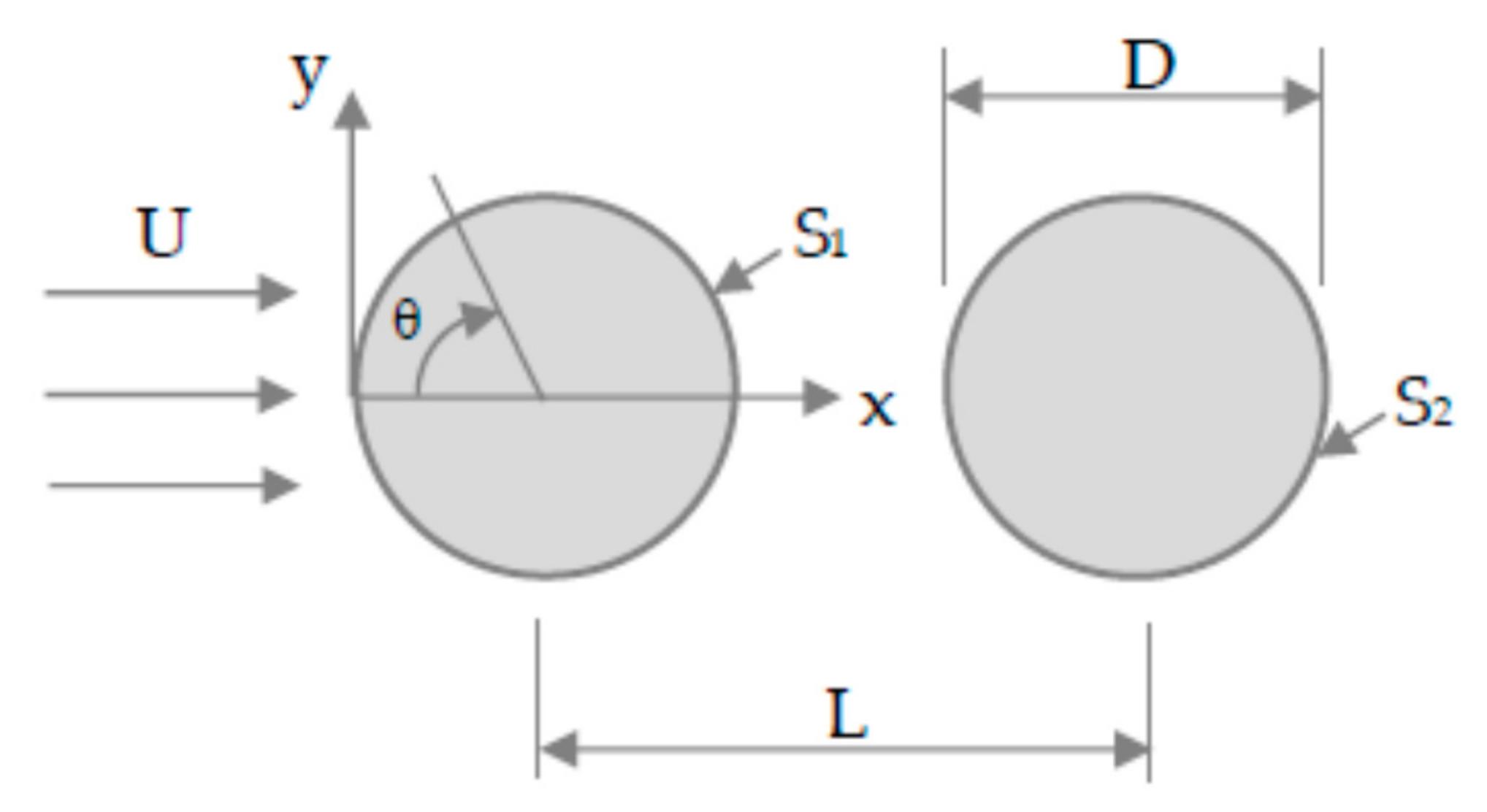
| D | outer cylinder diameter |
| f | vortex shedding frequency |
| F2 | second-order velocity structure function of the filtered field |
| G | Green function |
| L | center-to-center distance between the two circular cylinders in tandem arrangement |
| N | number of vortex blobs around a vortex blob to evaluate the local eddy viscosity coefficient |
| NP | number of source flat panels |
| NR | number of “rough points” on each semicircle to compute the average velocity differences |
| NV | number of vortex blobs that instantaneously construct the von Kármán vortex street |
| p | static pressure |
| P | random number for vorticity diffusion |
| Q | random number for vorticity diffusion |
| r | radial distance |
| Re | Reynolds number |
| Rec | “local” Reynolds number associated with turbulence modeling |
| St | Strouhal number |
| t | time |
| u | velocity field |
| U | inlet flow or freestream |
| x | position vector |
| Y | stagnation pressure |
| Z | number of vortex blobs to simulate radial diffusion of the vortical structure ΓV |
| ∆S | flat panel length |
| ∆t | time step |
| Γ | vortex blob strength |
| Γv | vortical structure strength or circulation |
| ∇ | Nabla operator |
| β | orientation angle of each flat panel |
| δ | position of generation of each vortex blob near a pivotal point |
| ε | size of a single roughness element |
| ζ | diffusive displacement of each vortex blob |
| θ | orientation angle of each pivotal point to computed pressure coefficient |
| ν | fluid kinematics viscosity coefficient |
| νt | local eddy viscosity coefficient |
| Ξ | fundamental solution of Laplace equation, |
| π | 3.14159… |
| ρ | fluid density |
| σ | source density |
| σ0 | Lamb vortex core |
| ω | vorticity |
| Ω | fluid domain |
References
- Zdravkovich, M.M. The effect of interference between circular cylinders in cross flow. J. Fluids Struct. 1987, 1, 239–262. [Google Scholar] [CrossRef]
- Sumner, D. Two circular cylinders in cross flow: A review. J. Fluids Struct. 2010, 26, 849–899. [Google Scholar] [CrossRef]
- Alam, M.M.; Moriya, M.; Takai, K.; Sakamoto, H. Fluctuating fluid forces acting on two circular cylinders in a tandem arrangement at a subcritical Reynolds number. J. Wind Eng. Ind. Aerodyn. 2003, 91, 139–154. [Google Scholar] [CrossRef]
- Alam, M.M.; Elhimer, M.; Wang, L.; Jacono, D.L.; Wong, C.W. Vortex shedding from tandem cylinders. Exp. Fluids 2018, 59, 1–17. [Google Scholar] [CrossRef] [Green Version]
- Schewe, G.; van Hinsberg, N.P.; Jacobs, M. Investigation of the steady and unsteady forces acting on a pair of circular cylinders in cross flow up to ultra-high Reynolds numbers. Exp. Fluids 2021, 62, 176. [Google Scholar] [CrossRef]
- Bimbato, A.M.; Alcântara Pereira, L.A.; Hirata, M.H. Simulation of viscous flow around a circular cylinder near a moving ground. J. Braz. Soc. Mech. Sci. Eng. 2009, 31, 243–252. [Google Scholar] [CrossRef] [Green Version]
- Bimbato, A.M.; Alcântara Pereira, L.A.; Hirata, M.H. Development of a new Lagrangian vortex method for evaluating effects of surfaces roughness. Eur. J. Mech. B Fluids 2019, 74, 291–301. [Google Scholar] [CrossRef]
- Oliveira, M.A.; Moraes, P.G.; Andrade, C.L.; Bimbato, A.M.; Alcântara Pereira, L.A. Control and Suppression of Vortex Shedding from a Slightly Rough Circular Cylinder by a Discrete Vortex Method. Energies 2020, 13, 4481. [Google Scholar] [CrossRef]
- Bimbato, A.M.; Alcântara Pereira, L.A.; Hirata, M.H. Study of Surface Roughness Effect on a Bluff Body—The Formation of Asymmetric Separation Bubbles. Energies 2020, 13, 6094. [Google Scholar] [CrossRef]
- Alcântara Pereira, L.A.; Oliveira, M.A.; Moraes, P.G.; Bimbato, A.M. Numerical experiments of the flow around a bluff body with and without roughness model near a moving wall. J. Braz. Soc. Mech. Sci. Eng. 2020, 42, 129. [Google Scholar] [CrossRef]
- Moraes, P.G.; Oliveira, M.A.; Andrade, C.L.; Bimbato, A.M.; Alcântara Pereira, L.A. Effects of surface roughness and wall confinement on bluff body aerodynamics at large-gap regime. J. Braz. Soc. Mech. Sci. Eng. 2021, 43, 397. [Google Scholar] [CrossRef]
- Blevins, R.D. Applied Fluid Dynamics Handbook; Van Nostrand Reinhold Co.: Washington, DC, USA, 1984. [Google Scholar]
- Nishino, T. Dynamics and Stability of Flow past a Circular Cylinder in Ground Effect. Ph.D. Thesis, Faculty of Engineering Science and Mathematics, University of Southampton, Southampton, UK, 2007. [Google Scholar]
- Bearman, P.W. Vortex shedding from oscillating bluff bodies. Annu. Rev. Fluid Mech. 1984, 16, 195–222. [Google Scholar] [CrossRef]
- Kundu, P.K. Fluid Mechanics; Academic Press: Cambridge, MA, USA, 1990. [Google Scholar]
- Leonard, A. Vortex methods for flow simulation. J. Comput. Phys. 1980, 37, 289–335. [Google Scholar] [CrossRef]
- Katz, J.; Plotkin, A. Low Speed Aerodynamics: From Wing Theory to Panel Methods; McGraw Hill Inc.: New York, NY, USA, 1991. [Google Scholar]
- Lesieur, M.; Métais, O. New trends in large eddy simulation of turbulence. Rev. Fluid Mech. 1996, 28, 45–82. [Google Scholar] [CrossRef]
- Batchelor, G.K.A. Introduction to Fluid Dynamics; Cambridge University Press: Cambridge, MA, USA, 1967. [Google Scholar]
- Chorin, A.J. Numerical study of slightly viscous flow. J. Fluid Mech. 1973, 57, 785–796. [Google Scholar] [CrossRef]
- Shintani, M.; Akamatsu, T. Investigation of two-dimensional discrete vortex method with viscous diffusion model. CFD J. 1994, 3, 237–254. [Google Scholar] [CrossRef] [Green Version]
- Ferziger, J.H. Numerical Methods for Engineering Application; John Wiley & Sons, Inc.: Hoboken, NJ, USA, 1981. [Google Scholar]
- Helmholtz, H. On integrals of the hydrodynamics equations which express vortex motion. Philos. Mag. 1867, 33, 485–512. [Google Scholar] [CrossRef]
- Chorin, A.J.; Hald, O. Stochastic Tools for Mathematics and Science, 3rd ed.; Springer: Berlin/Heidelberg, Germany, 2013. [Google Scholar]
- Lewis, R.I. Vortex Element Methods, The Most Natural Approach to Flow Simulation—A Review of Methodology with Applications. In Proceedings of the 1st International Conference on Vortex Methods, Kobe, Japan, 4–5 November 1999; pp. 1–15. [Google Scholar]
- Smagorinsky, J. General circulation experiments with the primitive equations. Mon. Weather Rev. 1963, 91, 99–164. [Google Scholar] [CrossRef]
- Achenbach, E. Influence of surface roughness on the cross-flow around a circular cylinder. J. Fluid Mech. 1971, 46, 321–335. [Google Scholar] [CrossRef]
- Achenbach, E.; Heinecke, E. On vortex shedding from smooth and rough cylinders in the range of Reynolds numbers 6 × 10³ to 5 × 10⁶. J. Fluid Mech. 1981, 109, 239–251. [Google Scholar] [CrossRef]
- Guven, O.; Farell, C.; Patel, V.C. Surface roughness effects on the mean flow past circular cylinders. J. Fluid Mech. 1980, 98, 673–701. [Google Scholar] [CrossRef]
- Ogami, Y.; Ayano, Y. Flows around a circular cylinder simulated by the viscous vortex method model—the diffusion velocity method. Comp. Fluid Dyn. J. 1995, 4, 383–399. [Google Scholar]
- Mustto, A.A.; Hirata, M.H.; Bodstein, G.C.R. Vortex method simulation of the flow around a circular cylinder. AIAA J. 1998, 38, 1100–1102. [Google Scholar]
- Gerrard, J.H. The mechanics of the formation region of vortices behind bluff bodies. J. Fluid Mech. 1966, 25, 401–413. [Google Scholar] [CrossRef]
- Rezek, T.J.; Camacho, R.G.R.; Filho, N.M.; Limacher, E.J. Design of a hydrokinetic turbine diffuser based on optimization and computational fluid dynamics. Appl. Ocean Res. 2021, 107, 102484. [Google Scholar] [CrossRef]
- Camacho, R.G.R.; Manzanares Filho, N. A source wake model for cascades of axial flow turbomachines. J. Braz. Soc. Mech. Sci. Eng. 2005, 27, 288–299. [Google Scholar]


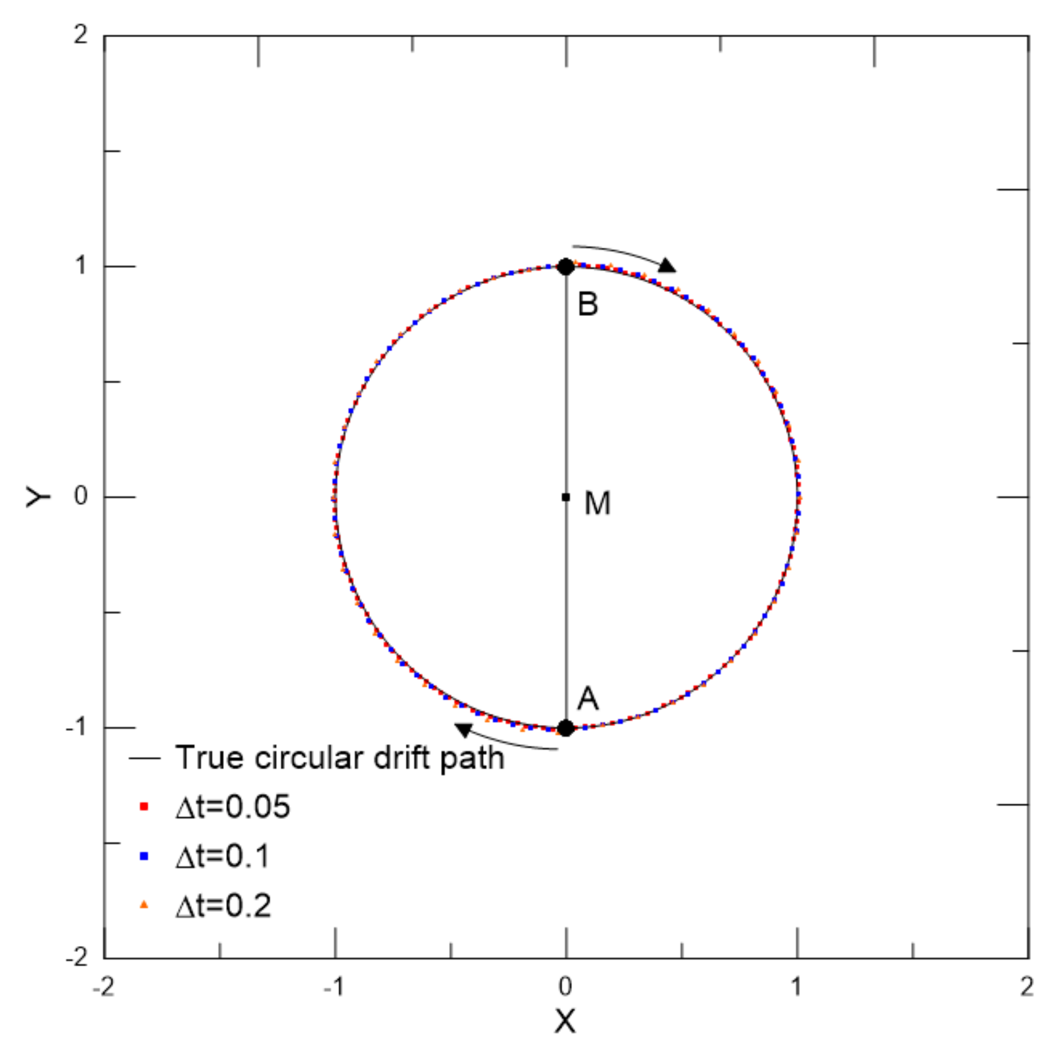
| Distance AB (Figure 3) | ΓA | σ0 | ∆t | Steps | Error (%) |
|---|---|---|---|---|---|
| 2.0D | 1.0 | 0.001D | 0.05 | 795 | 0.4406 |
| 2.0D | 1.0 | 0.001D | 0.1 | 400 | 0.8780 |
| 2.0D | 1.0 | 0.001D | 0.2 | 203 | 1.7478 |
| Case | CD | CL | St |
|---|---|---|---|
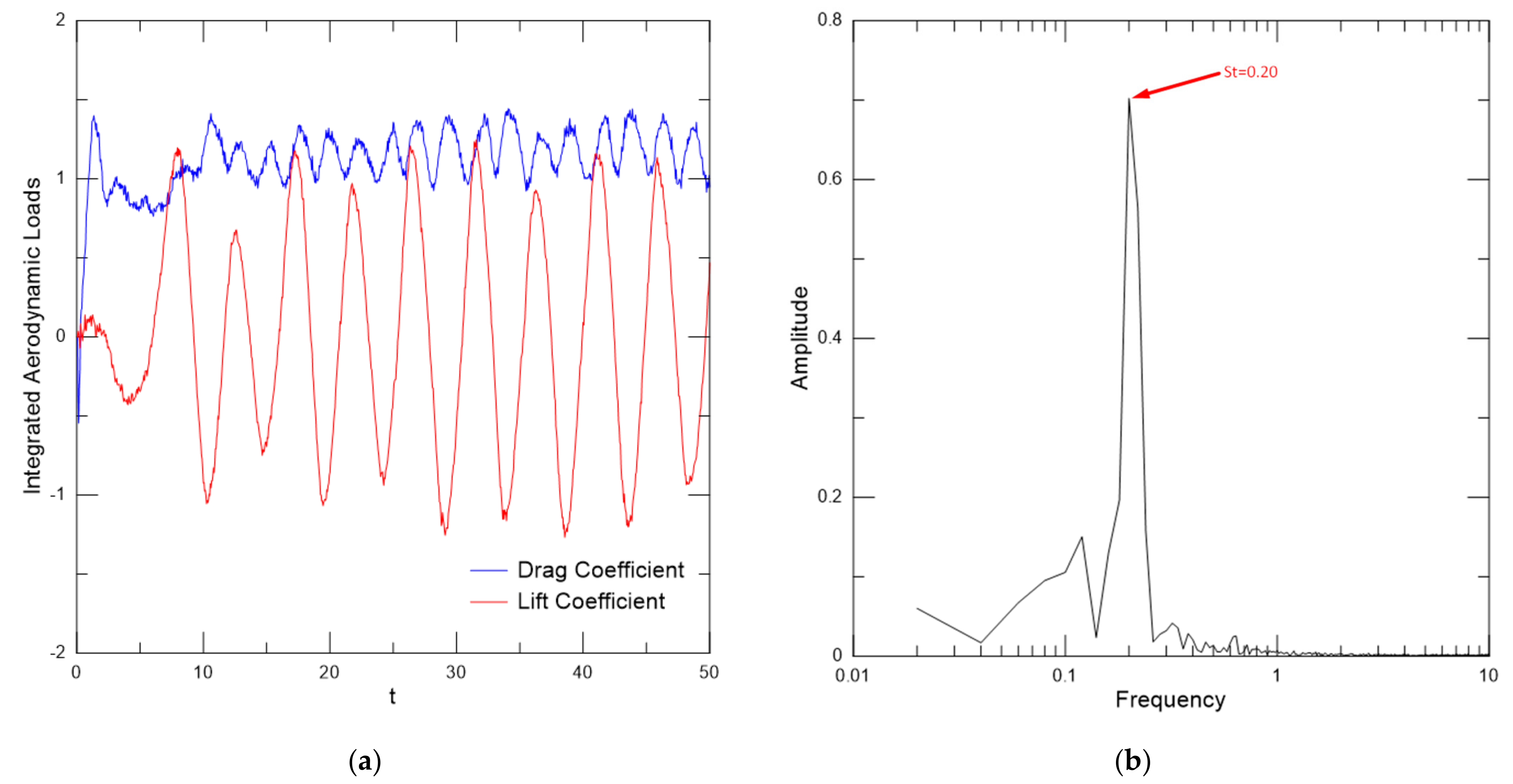
| Experimental [12] | 1.2000 | − | 0.1900 |
| Numerical [20] | 1.0700 | − | − |
| Numerical [30] | 1.1000 | − | − |
| Numerical [31] | 1.2200 | − | 0.2200 |
| Present simulation | 1.1873 | −0.0152 | 0.2000 |
| Case | Upstream Cylinder | Downstream Cylinder | ||||
|---|---|---|---|---|---|---|
| ε/D | CD | St | ε/D | CD | St | |
| Experimental [3] | − | 1.2612 | 0.1867 | − | 0.2766 | 0.1867 |
| Present Simulation | 0.000 | 1.0790 | 0.2000 | 0.000 | 0.4897 | 0.2000 |
| Present Simulation | 0.000 | 1.1035 | 0.2000 | 0.001 | 0.4409 | 0.2000 |
| Present Simulation | 0.001 | 0.9245 | 0.1875 | 0.000 | 0.6450 | 0.1875 |
| Present Simulation | 0.001 | 0.9018 | 0.1875 | 0.001 | 0.5060 | 0.1875 |
| Case | Upstream Cylinder | Downstream Cylinder | ||||
|---|---|---|---|---|---|---|
| ε/D | CD | St | ε/D | CD | St | |
| Experimental [3] | − | 1.2612 | 0.1867 | − | 0.2766 | 0.1867 |
| Present Simulation | 0.000 | 1.0790 | 0.2000 | 0.000 | 0.4897 | 0.2000 |
| Present Simulation | 0.000 | 1.0321 | 0.2000 | 0.007 | 0.3798 | 0.2000 |
| Present Simulation | 0.007 | 0.9904 | 0.2000 | 0.000 | 0.4860 | 0.2000 |
| Present Simulation | 0.007 | 1.0246 | 0.1875 | 0.007 | 0.4194 | 0.1875 |
Publisher’s Note: MDPI stays neutral with regard to jurisdictional claims in published maps and institutional affiliations. |
© 2021 by the authors. Licensee MDPI, Basel, Switzerland. This article is an open access article distributed under the terms and conditions of the Creative Commons Attribution (CC BY) license (https://creativecommons.org/licenses/by/4.0/).
Share and Cite
Moraes, P.G.d.; Alcântara Pereira, L.A. Surface Roughness Effects on Flows Past Two Circular Cylinders in Tandem Arrangement at Co-Shedding Regime. Energies 2021, 14, 8237. https://doi.org/10.3390/en14248237
Moraes PGd, Alcântara Pereira LA. Surface Roughness Effects on Flows Past Two Circular Cylinders in Tandem Arrangement at Co-Shedding Regime. Energies. 2021; 14(24):8237. https://doi.org/10.3390/en14248237
Chicago/Turabian StyleMoraes, Paulo Guimarães de, and Luiz Antonio Alcântara Pereira. 2021. "Surface Roughness Effects on Flows Past Two Circular Cylinders in Tandem Arrangement at Co-Shedding Regime" Energies 14, no. 24: 8237. https://doi.org/10.3390/en14248237
APA StyleMoraes, P. G. d., & Alcântara Pereira, L. A. (2021). Surface Roughness Effects on Flows Past Two Circular Cylinders in Tandem Arrangement at Co-Shedding Regime. Energies, 14(24), 8237. https://doi.org/10.3390/en14248237