Dynamic Modelling and Validation of an Air-to-Water Reversible R744 Heat Pump for High Energy Demand Buildings

Abstract

This paper presents a reversible heat pump based on CO₂ as the refrigerant, able to provide heating, cooling, and domestic hot water to high energy demand buildings. The unit was developed and tested under the EU H2020 project MultiPACK, which has the main goal of assuring the market about the feasibility, reliability, and energy efficiency of CO₂ integrated systems for heating and cooling and promoting a fast transition to low environmental impact solutions. Within the project, the confidence raising was performed by installation and monitoring of fully integrated state-of-the art CO₂ systems in the Southern European Climate. With the aim of predicting the unit behaviour under variable load and boundary conditions, a dynamic model of the entire unit was developed with commercial software, considering actual components and the implemented control system and it was validated with experimental data, collected at the factory’s lab before commissioning. The validation against experimental data collected during operation as a heat pump demonstrated a maximum percentage difference between the experimental and predicted value of gas–cooler heat flow rate equal to +5.0%. A preliminary comparison with the experimental data in chiller configuration is reported, however further development was required to achieve a satisfactory validation. Lastly, the numerical model was utilized to simulate a typical operation in heat pump configuration with the system coupled with a hot water tank storage for the production of domestic hot water and space heating; the model predicts higher COP when operating in domestic hot water operation due to the lower water inlet temperature.

1. Introduction

The European Commission [1] has recently confirmed that a renovation wave is needed to green the EU building stock, buildings being responsible for about 40% of the EU’s total energy consumption and for 36% of its greenhouse gas emissions from energy. One of the key principles for building renovation towards 2030 and 2050 is energy efficiency, which is classified by EU as the “horizontal guiding principle of European climate and energy governance and beyond to make sure we only produce the energy we really need”. According to the same communication, one of the seven areas of intervention is the decarbonisation of heating and cooling. The heating sector offers significant opportunities to decarbonise the energy business [2] and heat pumps appear as one of the most promising way to lower the carbon footprint of the heating system.

The push towards heat pump technology in place of fossil fuels for heating purposes, as previously described, together with the need for a long-term environmentally sustainable refrigerant solution, inspired by regulations, as F-gas regulation in Europe, and international protocols, such as the Kigali amendment to the Montreal Protocol, has stimulated research and industry towards the use of CO₂ also in heat pumps for comfort heating and cooling. Among the firsts, Heinz et al., 2010, [3] demonstrated that CO₂ might offer an efficient solution if low temperature heating is required, especially if applied to low-energy buildings.

In fact, since the revival of CO₂ as a refrigerant [4,5], CO₂ transcritical cycles have widely proved to be an energy efficient option for tap water heat pumps. The gas cooling process well fits with the warming up of a finite stream of water, resulting in a quite large temperature lift of the hot water produced without significant penalisation in Coefficient of Performance (COP), as was clearly demonstrated in the technical literature [6].

However, especially when retrofitting takes places, the temperature of water flowing back to the gas cooler, where heating takes place, might be high enough to be detrimental to the energy efficiency of the CO₂ transcritical cycle.

Aware of the intrinsic efficiency challenges, which might occur with the transcritical cycle at high return temperatures due to the temperature levels of the heat rejection fluid, it is important to properly design the system. In recent years, when extending the use of carbon dioxide as a refrigerant for commercial refrigeration systems in warm countries, many solutions to reduce expansion losses have been developed and installed, such as parallel compression, and experience has been consolidated. Some of these solutions can be easily adopted in chillers and heat pumps, taking into consideration the specificity of the heating and cooling sector. Two-phase ejectors have been identified as a simple way to recover part of the expansion work for recirculation and precompression, still maintaining a simple design, as proposed in Lorentzen, 1984 [7]. By theoretical [8] and experimental assessments [9,10], the use of ejectors have become a state-of-the art technology in CO₂ refrigeration [11].

When simultaneous heating and cooling is required, CO₂ systems offer good efficiency [12]. Heat recovery for space heating is also common practice, as it has been happening for a long time in CO₂ commercial refrigeration plants, representing the best example of simultaneous heating and cooling.

Minetto et al., 2016 [13] simulated the performances of a reversible CO₂ unit intended for heating, cooling, and hot water in a residential building. They demonstrated that, with the use of an ejector in place of the expansion valve, the CO₂ system could equal the performance of an R410A unit, despite the fact that, due to the technology development at the time, a water to water system was required to reverse the system in the CO₂ layout.

Amongst other buildings, hotels are relevant energy consumers. According to Styles et al., 2017 [14] the contribution of the accommodation sector to global CO₂ emissions related to energy consumption is 1%. According to the same report, the energy related to heating, cooling, ventilation, and DHW in hotels accounts for more than 65%, with 17% of this from DHW; about 55% of the total energy requirement relies on fossil fuels.

By merging the needs of high energy demanding buildings, e.g., hotels, with the achievements in the use of CO₂ as a refrigerant also in heat pumps, the EU funded project MultiPACK meets the challenge of installing integrated units for heating, cooling, and DHW production, based on CO₂, and adopting two-phase ejectors to improve efficiency at high gas–cooler outlet temperature.

MutiPACK has the main goal of installing six units in the field, including three units for hotels, able to satisfy the energy needs with a high standard of environmental sustainability. These units are fully monitored to prove the performances in the field, thus increasing the confidence of stakeholders in the technical solutions and also helping in overcoming nontechnological barriers that can hinder the adoption of available energy efficient solutions in the HVAC&R sector, as demonstrated by the SuperSmart EU project [15].

Dynamic modelling of the vapour compression system has been widely explored in the literature; Bryan et al. [16] provides a comprehensive review of both physical and databased approaches for transient simulation of refrigeration systems, pointing out how experimental validation of such models is essential and concluding with a more useful perspective for physical models.

CO₂ cycles introduce a higher complexity in the layout design and the need for the further control of high pressure. Rasmussen, 2005 [17] presented the transient model of a carbon dioxide transcritical cycle, where the heat exchangers adopted the moving-boundary approach; the model was validated experimentally. Shi et al., 2010 [18], developed a dynamic model of a transcritical CO₂ cooling unit using the commercial software Dymola to assess the system performance in the absence of physical prototypes. In the same year, Gräber et al., 2010 [19] presented a new library for Dymola that was used to simulate and validate the dynamic model of a CO₂ heat pump.

Zheng et al., 2015 [20] developed a transient model of a CO₂ transcritical cycle equipped with an ejector, assuming a 1-D two-phase ejector model, and they evaluated the response of the system to different expansion valve opening degree and area ratios of the ejector.

Barta et al., 2019 [21] recently presented the dynamic simulation of a three-stage compression, two-level evaporation CO₂ cycle for military applications, under extreme environmental conditions. The model was developed with Dymola/Modelica language and used to investigate the control system.

Artuso et al., 2020 [22] developed a numerical model of a CO₂ system for road transport refrigeration, using the software AMESim; the energy performance was discussed for different values of internal space temperature and external ambient temperature.

In this paper, pre-commissioning tests of the MultiPACK unit for hotels, carried out at the factory’s facilities, are used to validate a dynamic model of the unit, including all its components, i.e., two compressors in parallel, four CO₂/water heat exchangers, and a CO₂/air heat exchanger. Considering the complexity and the size of the MultiPACK units, which make experimental activity expensive and time consuming, the model can offer a useful tool to different purposes. Forecasting the performance of the system in a reliable and affordable way, once boundaries are defined, such as thermal load profiles and outdoor temperature, or testing different control logic for operation optimisation and energy consumption minimisation are crucial to promote the successful diffusion of CO₂ based, environmentally friendly HVAC units for high energy consumption buildings. The model was developed with the software AMESim.

2. The System Layout and the Experimental Setup

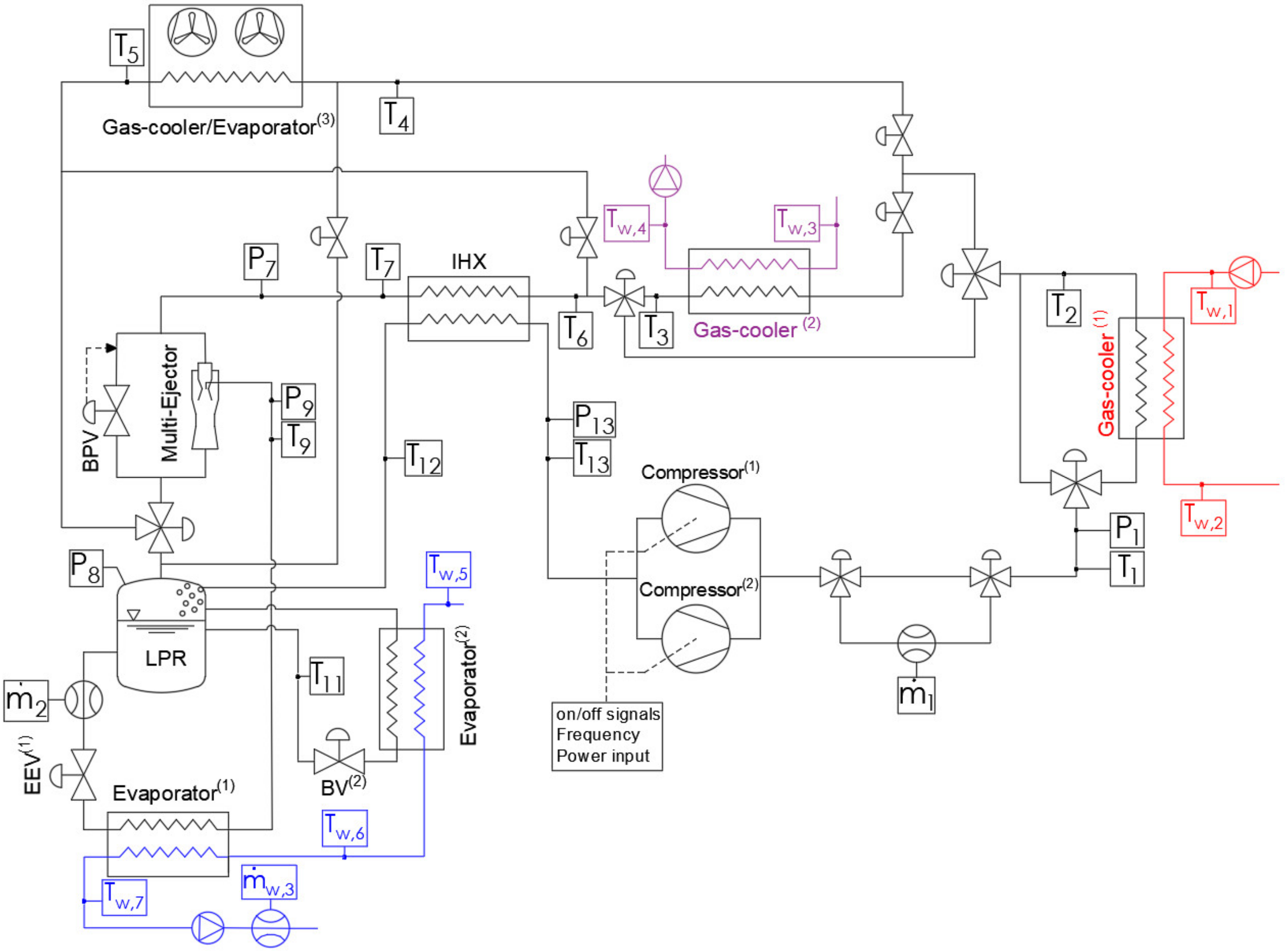
The scheme of the refrigerating system is provided in Figure 1, while the main component characteristics are listed in

Table 1. Geometric dimensions of the system main components as named in Figure 1.

Component	Geometric Dimensions/Characteristics
Compressors(1) Compressor(2)	Reciprocating, semi-hermetic, single stage compressor. Displacement volume 180.6 cm3 and 205.0 cm3. Allowable suction pressure: $14.3 bar<p_{asp} < 50.8 bar$; Maximum discharge pressure: $p_{discharge}<135 bar$
Gas-cooler(1)	Counter flow, single pass brazed-plate heat exchanger. Heat transfer area of 8.90 m2
Gas-cooler(2)	Counter flow, single pass brazed-plate heat exchanger. Heat transfer area of 7.42 m2
IHX	Counter flow, tube-in-tube type heat exchanger. Heat transfer area: Low pressure side 0.20 m2, high pressure side 0.22 m2
Gas-cooler/Evaporator	Finned coil heat exchanger, external area 491.00 m2, internal area 62.4 m2.
LPR	Low pressure receiver. Internal volume of 0.155 m3
Evaporator(1)	Counter flow, single pass brazed-plate heat exchanger. Heat transfer area of 7.62 m2
Evaporator(2)	Counter flow, single pass brazed-plate heat exchanger. Heat transfer area of 10.90 m2
BPV	Electrically operated step motor valve. Maximum opening diameter 4.8 mm
EEV(1)	Electrically operated step motor valve. Maximum opening diameter 9.5 mm

. The unit has two semi-hermetic compressors (compressor⁽¹⁾ and compressor⁽²⁾), two brazed-plate gas-coolers (gas-cooler⁽¹⁾ and gas-cooler⁽²⁾), a finned-coil heat exchanger (gas-cooler/evaporator⁽³⁾), an internal heat exchanger (IHX) between the compressor suction line and gas-cooler outlet line, a back-pressure valve (BPV), a multi-ejector rack, a low-pressure receiver (LPR), and an electronic expansion valve (EEV⁽¹⁾). The operation of the system can be switched between two main configurations, i.e., heat pump and chiller, by means of circulation valves located in the circuit.

As the refrigerating system is utilized for the production of chilled and hot water in different operating conditions, a more complex configuration was presented compared to the traditional solution. In particular, the system is capable of operating according to a heat pump configuration, for the production of domestic hot water and space heating, and as a chiller configuration for the production of chilled water and eventually hot water. The heat pump configuration consists of a simple configuration air/water heat pump, where the heat is absorbed by the finned coil evaporator and rejected to the brazed plate gas-cooler in order to heat up the incoming water heat flow rate. On the other hand, the chiller configuration has a more complicated operating scheme: a parallel between the back-pressure valve and a multi-ejector system can be employed for the expansion of the refrigerant, to feed an ejector driven evaporator (Evaporator⁽¹⁾) and a natural circulation evaporator (Evaporator⁽²⁾), which cool down a water stream matching the temperature profile. An extra brazed-plate gas-cooler is included for domestic hot water production.

Table 2. Accuracy of the instruments.

Measurement	Instrument	Accuracy
Power	Three phase network analyser and current transformer	0.5% FS (FS = 130 kW)
Temperature	T-type thermocouple	±0.2 K
Pressure	Pressure transducer	±0.24 bar
Mass flow rate, CO2	Coriolis flowmeter	±0.1% reading (liquid) ±0.5% reading (vapour)
Mass flow rate, water	Electromagnetic flowmeter	1% reading

reports the accuracy of the instruments used to monitor the system.

2.1. Heat Pump Configuration

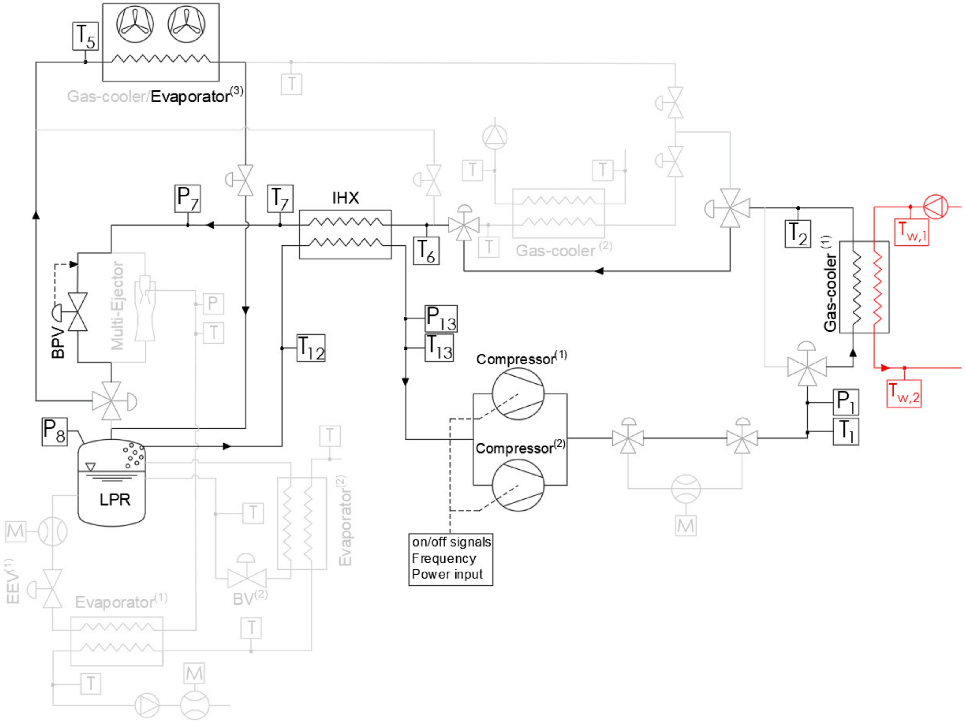
During operation as a heat pump, CO₂ is compressed by the two semi-hermetic compressors. One of the compressors is inverter controlled, based on water outlet temperature, while the other compressor operates at a fixed speed. After the compression, the refrigerant in a supercritical state flows in a single-pass brazed-plate gas-cooler before entering the high-pressure side of the internal heat exchanger where it is further cooled down. The refrigerant is then expanded to the evaporation pressure by a back-pressure valve, whose cross-section is modulated by a PI controller to maintain the design high-pressure value $p_{HP}^{set-point}$, before flowing into the low pressure receiver (LPR) after the evaporation.

The internal heat exchanger (IHX) provides saturated vapour superheating before compression. The simple heat pump configuration is reported in Figure 2.

2.2. Chiller Configuration

When operating according to the chiller configuration, the system features two evaporators, according to a patented design (EP3486580). One evaporator is fed from the liquid separator, thanks to natural circulation; the flow in the second evaporator is driven by the two-phase ejector block, thus bringing a lower saturation temperature. Purely for testing purposes, the unit can be forced to operate with a single compressor and the ejector driven evaporator, closing the valve BV⁽¹⁾, thus resulting in the reference ejector layout [4]. The unit standard configuration includes two evaporators and compressors, whose capacity is controlled on cold water delivery temperature, by acting on compressors on/off and inverter frequency.

2.2.1. Single Compressor and Single Evaporator

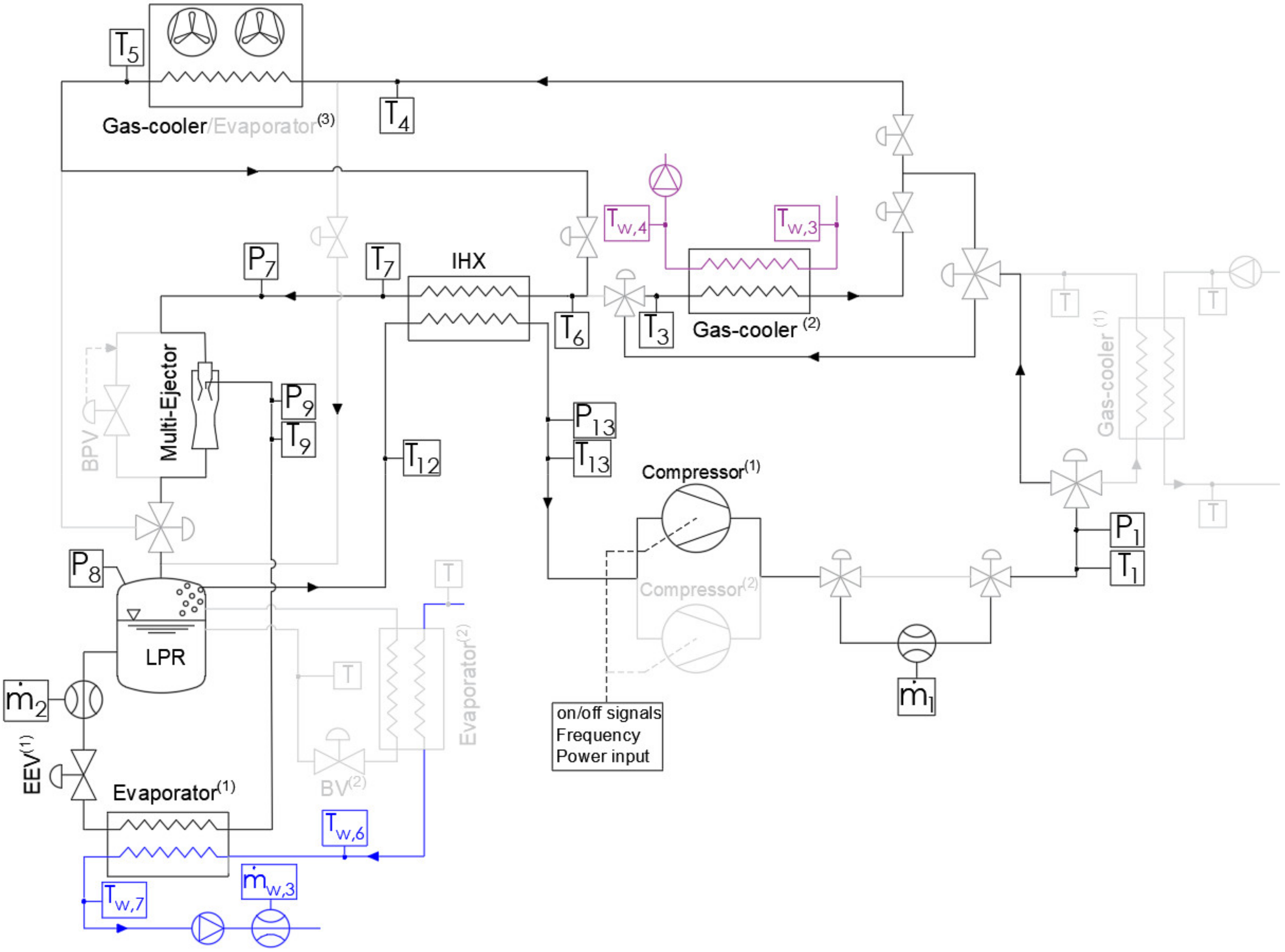
Figure 3 reports the schematic of the refrigerating system operating according to the chiller configuration with a single compressor and a single evaporator. When operating in this configuration the refrigerant is compressed to the transcritical state with a single compressor operating at fixed speed. A brazed plate gas-cooler (gas-cooler⁽²⁾) can be utilized for the hot water production (though it can be bypassed) and the refrigerant is further cooled down in the finned coil gas-cooler. The finned coil fans rotation speed is modulated by a PI controller in order to optimise the temperature at the gas-cooler’s outlet, $T_{out-gc}^{set-point}$. After flowing into the high pressure side of the internal heat exchanger, the refrigerant streams through the motive nozzle, and is expanded in the multi-ejector rack, which has also the role of maintaining the high pressure set point $p_{HP}^{set-point}$, while the back-pressure valve is kept closed. The refrigerant in the state of saturated liquid flows through the expansion valve (EEV⁽¹⁾), whose opening degree is decided by a PI controller in order to maintain a certain set-point pressure at the low-pressure receiver $p_{LPR}^{set-point}$, and is expanded to the evaporation pressure, before flowing into the brazed-plate evaporator (Evaporator⁽¹⁾). The refrigerant exiting the evaporator is recirculated by the ejector rack back to the LPR.

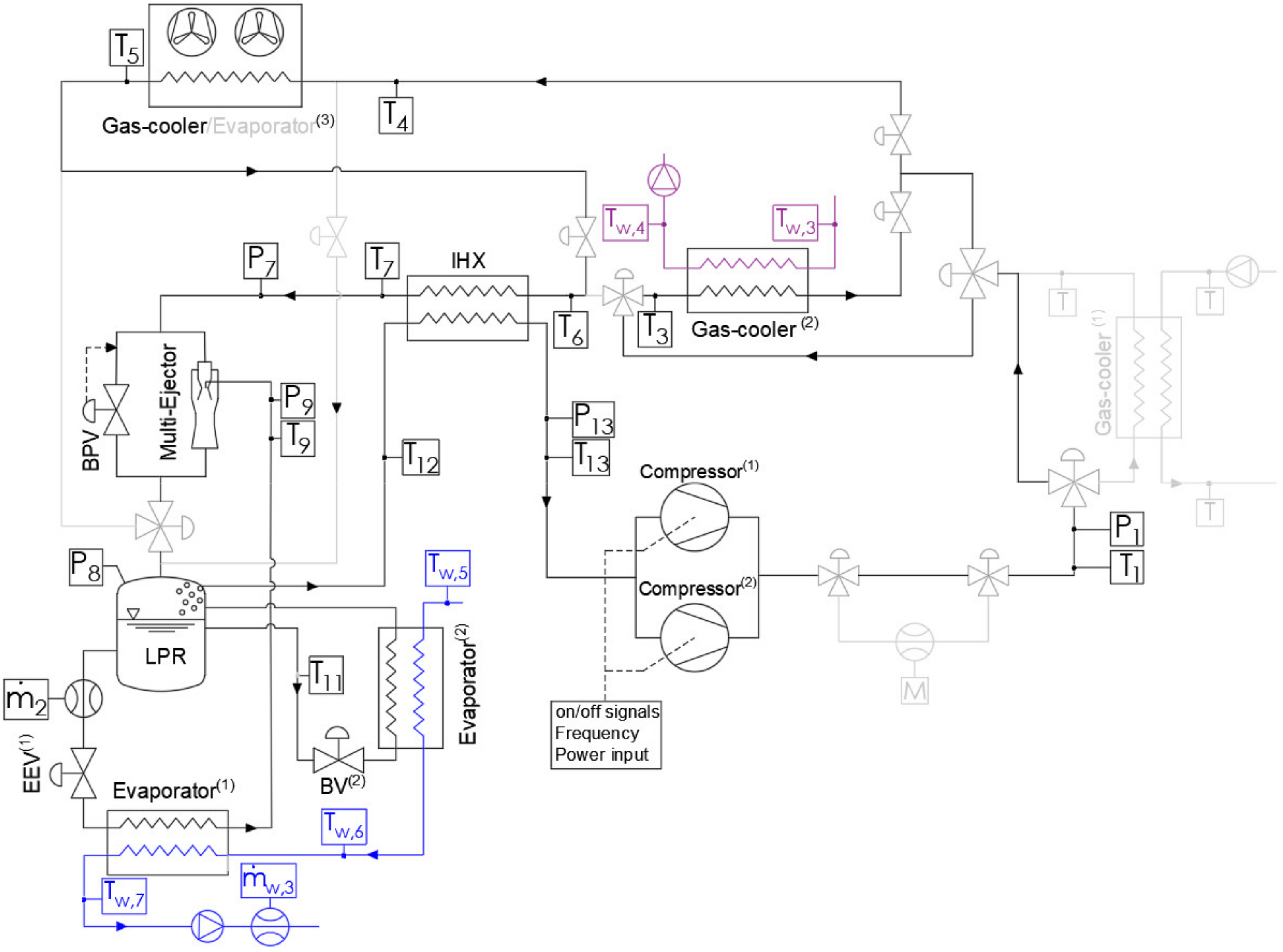
2.2.2. Two Compressors and Two Evaporators

The standard operation model of the chiller includes both semi-hermetic compressors and two evaporators, including the flooded evaporator (Evaporator⁽²⁾). The operation of this configuration is similar to the previous one, however, the additional semi-hermetic compressor is inverter controlled (compressor⁽²⁾) on the water outlet temperature. Furthermore, the expansion of the refrigerant is achieved with a parallel between a back-pressure valve (BPV) and the multi-ejector system. The multi-ejector and the BPV are controlled to maintain the set-point high pressure $p_{HP1}^{set-point}$. The two compressors, two evaporators system configuration is reported in Figure 4.

2.2.3. Data Reduction

Experimental data were collected during the operation in steady-state conditions of the refrigerating system in heat pump and chiller configurations. When operating according to the heat pump configuration, the heat flow rate at the gas-cooler was derived on refrigerant side (Equation (1)).

$${\dot{Q}}_{g{c}_{\left(1\right)}}^{{\mathrm{CO}}_2}={\dot{m}}_{{\mathrm{CO}}_2}\left(h_1-h_2\right)$$

(1)

When the system was operating with both semi-hermetic compressors, CO₂ mass flow rate was not measured by the Coriolis meter, due to its limited FS. The performance of each compressor was then validated against the manufacturer’s polynomials independently from the other, with dedicated tests considering different compressor ratio and frequencies. In Figure 5a, the mass flow rate is reported for both the fixed speed and the inverter controlled compressor. Percentage errors were on average 3%, which is within the tolerance admitted by EN12900:2013 for mass flow declared data and the measurement accuracy.

These tests were also used to verify the polynomial curves describing the overall compressor efficiency, thus, the compressor power consumption. When the fixed speed compressor was considered, the experimental reading could be directly compared to the manufacturer’s data. On the other side, in the case of inverter controlled compressor, we have to account for the inverter efficiency. This was assumed to be 95%, according to the inverter data sheet.

Figure 5b presents the same operating points of Figure 5a in terms of nominal against experimental electrical power consumption. For both the compressors, the power was systematically underestimated by the nominal data. For each frequency lower than 50 Hz, the average error was 5.8%, which is consistent with the tolerance allowed for data declaration (5% according to EN12900:2013) and the measurement accuracy. The 60 Hz actual power was 10.5% higher than the expected. This can be ascribed to a drop in the compressor efficiency at higher speeds and/or a decrease in the inverter performances. This aspect will need further investigation.

The heat flow rate at the internal heat exchanger (Equation (4)), was evaluated as the average value of the heat flow rate in the high (Equation (2)) and low pressure (Equation (3)) side of the heat exchanger.

$${\dot{Q}}_{IHX}^{HP}={\dot{m}}_{{\mathrm{CO}}_2}\left(h_6-h_7\right)$$

(2)

$${\dot{Q}}_{IHX}^{LP}={\dot{m}}_{{\mathrm{CO}}_2}\left(h_{12}-h_{13}\right)$$

(3)

$${\dot{Q}}_{IHX }=\frac{{\dot{Q}}_{IHX}^{HP}+{\dot{Q}}_{IHX}^{LP}}{2}$$

(4)

The COP of the heat pump was calculated according to Equation (5).

$$CO{P}_{heat-pump}=\frac{{\dot{Q}}_{g{c}_{\left(1\right)}}}{P_{el,comp}}$$

(5)

When the system was operating in chiller configuration, the heat flow rate at the gas-cooler⁽²⁾ was evaluated according to (Equation (6)):

$${\dot{Q}}_{g{c}_{\left(2\right)}}^{{\mathrm{CO}}_2}={\dot{m}}_{{\mathrm{CO}}_2}\left(h_3-h_4\right)$$

(6)

The heat flow rate at the finned coil gas-cooler was evaluated according to Equation (7):

$${\dot{Q}}_{g{c}_{\left(3\right)}}={\dot{m}}_{{\mathrm{CO}}_2}\left(h_4-h_5\right)$$

(7)

Lastly, the heat flow rate at the brazed-plate evaporator⁽¹⁾ was evaluated according to (Equation (8)), when the refrigerant at the evaporator⁽¹⁾ outlet was in a superheated state.

$${\dot{Q}}_{ev{a}_{\left(1\right)}}^{{\mathrm{CO}}_2}={\dot{m}}_{sn}\left(h_{SL}-h_9\right)$$

(8)

When the refrigerant was in a two-phase state, the heat flow rate at the evaporator was evaluated with (Equation (9)), as the refrigerant enthalpy at evaporator outlet was not defined using pressure and temperature at point 9:

$${\dot{Q}}_{ev{a}_{\left(1\right)}}^w={\dot{m}}_{w,3}\left(h_{w,6}-h_{w,7}\right)$$

(9)

As for the evaporator⁽²⁾, the heat flow rate at the evaporator was given only on the water side (Equation (10)), as the refrigerant mass flow was not available.

$${\dot{Q}}_{ev{a}_{\left(2\right)}}^w={\dot{m}}_{w,3}\left(h_{w,5}-h_{w,6}\right)$$

(10)

The coefficient of performance of the system operating according to the chiller configuration was then given by Equation (11).

$$CO{P}_{chiller}=\frac{{\dot{Q}}_{ev{a}_{\left(1\right)}}+{\dot{Q}}_{ev{a}_{\left(2\right)}}}{P_{el,comp}}$$

(11)

Table 3. Maximum uncertainties of the main heat flow rate evaluation.

	Evaluation Method	Max Uncertainty [%]
${\dot{Q}}_{gc}^{}$	CO2 side	5.0
${\dot{Q}}_{IHX}$	CO2 side	5.5
${\dot{Q}}_{eva}$	CO2 side	0.7
	Water side	16.0

summarises the maximum uncertainties evaluated during the experiments presented in Section 4; on the high pressure side, whenever the heat flow was calculated on CO₂ side, the uncertainty related to the CO₂ mass flow calculation with compressor curves was always applied, in favour of safety. In the case of the calculation performed on the water side, which occurred whenever the evaporator exit was not superheated, the uncertainty was heavily affected by the very limited water temperature difference.

3. Numerical Model Development

After the experimental characterization of the refrigerating system operating according to the different configurations, the mathematical model of the system was developed with the commercial software Simcenter AMESim v.17. The libraries of the software are composed of basic elements designed to model the transient behaviour of the internal and external flows, i.e., refrigerant, air and water.

On the refrigerant side, components were modelled based on a homogeneous fluid model, i.e., the two-phase flow was considered as a single phase fluid, displaying the mean fluid properties. Refrigerant and water pressure losses and heat transfer coefficients were evaluated with empirical correlations from the literature. In addition, the model neglected the effect of gravity; the natural convection heat exchanger was thus neglected in this work and preliminary results of the chiller configuration will be presented including only the ejector driven evaporator. The two-phase flow library provided the thermophysical properties of carbon dioxide, water, and air; the thermodynamic properties of CO₂ were evaluated with the Modified Benedict Webb Rubin (MBWR) equation [23], considering the pressure as a function of the fluid’s density and temperature. Water was assumed to be pure and its thermodynamic properties were calculated with Bode’s formulation, and air was considered as a mixture, composed of a combination of pure fluids weighted by their concentration.

Basic elements were coupled to develop the submodel of the main components of the system, which were connected to form the complete numerical model of the refrigerating unit. The system included mass flow devices (compressor, expansion devices, and two-phase ejector) and energy flow devices (evaporators, gas-coolers/condensers, and internal heat exchangers); as the dynamics of the mass flow devices are generally an order of magnitude faster than those of the heat exchangers, according to Rasmussen et al., 2005 [17], the compressor, expansion devices, and two-phase ejector were considered static components and were modelled using steady-state empirical equations. On the other hand, the modelling of the heat exchangers, which are characterized by a more complex nature, was conceived with a discretization of the devices into smaller volumes, each treated with a lumped parameters approach. Finally, the pressure drops of the refrigerant flowing through the pipes connecting different components was neglected, as the assumption of short pipes was made.

3.1. Low Pressure Receiver Numerical Model

The low-pressure receiver is a device used to separate liquid from the vapour, storing excess of refrigerant mass to ensure system capacity over a wide range of operating conditions while preventing liquid flow back and consequent damage to the compressor. The submodel of the liquid-vapour separator was conceived assuming an adiabatic constant cross-sectional area; pressure was assumed to be homogeneous in the entire volume and the densities of both the liquid and vapour phase were considered homogeneous as well in their respective volumes. The average refrigerant pressure ${\overline{p}}_{LPR}$ and specific enthalpy ${\overline{h}}_{LPR}$ were used to compute the state of the refrigerant leaving the receiver (in the state of saturated liquid and vapour, respectively) and the percentage of liquid volume $r_{LV}$ inside of the receiver, which was used to determine the height of the liquid–vapor interface $H_{LV}$.

3.2. Semi-Hermetic Compressor Numerical Model

The semi-hermetic compressor was modelled as a fixed-displacement compressor. The parameters required as input were the value of volumetric efficiency ${\eta }_{vol}$ and overall compression efficiency ${\eta }_{comp}$, which were computed from data supplied by the compressor manufacture, the compressor’s displacement $V_d$, and the nominal rotatory speed $n$.

The adherence of the nominal maps has been already discussed in Section 2.2.3, showing a good agreement in terms of mass flow rate and a systematic underestimation of the power consumption of 5%, which increased to 10% when the inverter was set to 60 Hz. As a complete experimental characterization of the compressors in all the working conditions is beyond the scope of this research, the nominal data were used to model the compressor, still being aware of the findings illustrated in Section 2.2.3. for the critical evaluation of the model accuracy. Given the state of the refrigerant at the inlet, the numerical model of the compressor provided the mass-flowrate developed (Equations (12) and (13)), electric power input (Equation (14)), and state of the refrigerant at the compressor outlet. In the case of the fixed speed compressor, which operated at the constant speed of 1450 rpm, the developed mass flow rate was evaluated with Equation (12). In the case of the variable speed compressor, the developed mass flow rate was evaluated with Equation (13) instead, where the value of frequency modulation between 30 and 60 Hz provided by the inverter, $Inv \in \left[0, 1\right]$ was considered.

$${\dot{m}}_{V,FIXED}={\rho }_{IN}\frac{n}{60}{V}_d{\eta }_{vol}$$

(12)

$${\dot{m}}_{V,INV}={\rho }_{IN}\frac{n}{60}{V}_d{\eta }_{vol}\frac{30+30 Inv}{50}$$

(13)

$$P_{el,comp}=\frac{{\dot{m}}_V\Delta h_{is}}{{\eta }_{comp}}$$

(14)

3.3. Heat Exchanger Numerical Model

The modelling of the heat exchangers was achieved with an approximation to a simple straight tube in perfect counter flow configuration in a similar manner as discussed in Artuso et al., 2020 [22]. The equivalent tube was characterized by the hydraulic diameter of the heat exchanger ($D_h=D_i$ for the finned coil heat exchanger and internal heat exchanger and $D_h=2b_p⁄{\varphi }_p$ for the brazed-plate heat exchanger) and the equivalent length which was calculated according to Equation (15).

$$L_{pipe}=\raisebox{1ex}{$A_{HX}{D}_h$}\!\left/ \!\raisebox{-1ex}{$4A_{c,tot}$}\right.$$

(15)

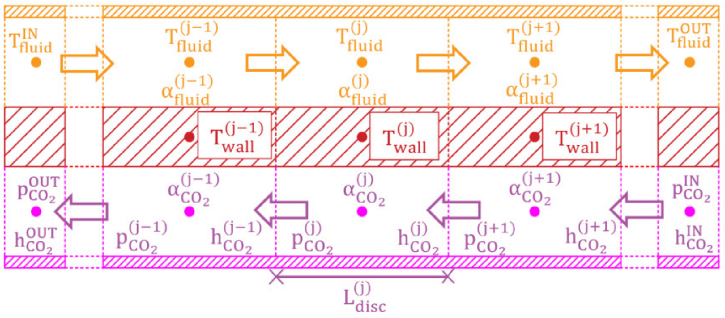
The equivalent pipe was then discretized into $N_{disc}$ elements (Figure 6), which was decided with a preliminary sensitivity study where $N_{disc}$ was increased until the solution demonstrated insensitivity to the variation of number of elements, and the length of the pipe and heat transfer area were equally distributed in each element.

For each discretized volume, it was possible to identify three nodes: a node referring to the refrigerant flow ($C_r$), a node referring to the state of the heat exchanger’s walls ($C_w$), and a node referring to the state of the air or water, respectively, $\left(C_a\right)$. The refrigerant and water flow were considered one-dimensional and the fluid properties varied only on the direction of the flow. In each discretized volume, the refrigerant pressure and density in the associated volume were computed according to Equations (16) and (17), which are given by the mass and energy balance equations applied to the j-th element:

$$V_r^{\left(j\right)}\left({\left.\frac{\partial {\overline{\rho }}_r }{\partial p}\right|}_h^{\left(j\right)}\frac{d{\overline{p}}_r^{\left(j\right)}}{dt}+{\left.\frac{\partial {\overline{\rho }}_r^{\left(j\right)}}{\partial h}\right|}_p^{\left(j\right)}\frac{d{\overline{h}}_r^{\left(j\right)}}{dt}\right)={\dot{m}}_r{}^{\left(j\right)}-{\dot{m}}_r{}^{\left(j-1\right)}$$

(16)

$$V_r^{\left(j\right)}\left[\left({\overline{h}}_r^{\left(j\right)}{\left.\frac{\partial {\overline{\rho }}_r}{\partial p}\right|}_h^{\left(j\right)}-1\right)\frac{d{\overline{p}}_r^{\left(j\right)}}{dt}+\left({\overline{h}}_r^{\left(j\right)}{\left.\frac{\partial {\overline{\rho }}_r}{\partial h}\right|}_p^{\left(i\right)}+{\overline{\rho }}_r^{\left(j\right)}\right)\frac{d{\overline{h}}_r^{\left(j\right)}}{dt}\right]={\dot{m}}^{\left(j-1\right)}{\overline{h}}_r^{\left(j-1\right)}-{\dot{m}}^{\left(j\right)}{\overline{h}}_r^{\left(j\right)}-{\dot{Q}}_{convi}^{\left(j\right)}$$

(17)

From the above equations, the trend of the mean thermodynamic properties of the refrigerant flowing inside the j-th tube element (${\overline{T}}_r^{\left(j\right)}$, ${\overline{p}}_r^{\left(j\right)}$,${\overline{h}}_r^{\left(j\right)}$) were obtained. The internal convective heat flux between the refrigerant and the wall of the heat exchanger in each element is given by Equation (18):

$${\dot{Q}}_{convi}^{\left(j\right)}={\alpha }_i^{\left(j\right)}{A}_i^{\left(j\right)}\left({\overline{T}}_w^{\left(j\right)}-{\overline{T}}_r^{\left(j\right)}\right)$$

(18)

where ${\alpha }_i$ is the internal convective heat transfer coefficient, computed from empirical correlations available in the literature, which will be explained later in this section. The thermal-capacity component accounting for the thermal structure of the heat exchanger quantifies the mean wall temperature ${\overline{T}}_w^{\left(j\right)}$ through Equation (19), obtained by the energy conservation equation with the assumption of monodimensional heat flow, as conduction heat flow through wall elements was neglected:

$$C_W^{\left(j\right)}\frac{d{\overline{T}}_W^{\left(j\right)}}{d\tau } ={\dot{Q}}_{convi}^{\left(j\right)}-{\dot{Q}}_{conve}^{\left(j\right)}$$

(19)

The external flow component assessed the mean thermodynamic properties of the air or water flowing outside of the j-th tube element (${\overline{T}}_a^{\left(j\right)}$, ${\overline{p}}_a^{\left(j\right)}$,${\overline{h}}_a^{\left(j\right)}$). In the case of water, the flow was assumed to be one dimensional as with the refrigerant flow, while in the case of air, zero-dimensional flow and negligible conduction in air flow direction was assumed. The convective heat flow of the external flow was computed through Equation (20).

$${\dot{Q}}_{conve}^{\left(j\right)}={\alpha }_e^{\left(j\right)}{A}_e^{\left(j\right)}\left({\overline{T}}_a^{\left(j\right)}-{\overline{T}}_W^{\left(j\right)}\right)$$

(20)

All the empirical correlations utilized in the refrigerant, air side, and water side in the heat exchangers of the system are listed in

Table 4. Empirical correlation utilized in the case of finned coil heat exchanger.

Applied Region	Items	Correlation
Air side	Heat transfer coefficient	Colburn j-factor [24]
Refrigerant side: evaporation	Heat transfer coefficient	Two-phase: VDI for horizontal tube, 1992 [25] Single phase: Gnielinski, 1976 [26]
	Pressure drop	Friedel, 1979 [27]
Refrigerant side: gas-cooling/condensation	Heat transfer coefficient	Transcritical: Gnielinski, 1976 [26] Subcritical: Shash, 1979 [28]
	Pressure drop	Friedel, 1979 [27]

,

Table 5. Empirical correlation utilized in the case of brazed-plate heat exchanger.

Applied Region	Items	Correlation
Water side	Heat transfer coefficient	Sieder and Tate, 1936 [29]
	Pressure drop	Friedel, 1979 [27]
Refrigerant side: evaporation	Heat transfer coefficient	Two-phase: Sieder and Tate, 1936 [29] Single phase: Sieder and Tate, 1936 [29]
	Pressure drop	Friedel, 1979 [27]
Refrigerant side: gas-cooling/condensation	Heat transfer coefficient	Transcritical: Sieder and Tate, 1936 [29] Subcritical: Sieder and Tate, 1936 [29]
	Pressure drop	Friedel, 1979 [27]

and

Table 6. Empirical correlation utilized in the case of internal heat exchanger.

Applied Region	Items	Correlation
Refrigerant side: gas-cooling/condensation	Heat transfer coefficient	Transcritical: Sieder and Tate, 1936 [29] Subcritical: Sieder and Tate, 1936 [29]
	Pressure drop	Friedel, 1979 [27]

.

The inputs required by the submodel were the geometric dimensions of the heat exchanger, and the state of the two fluids, i.e., refrigerant and air/water, at the inlet. The model evaluated, for each discretized element: the state of the refrigerant (${\overline{T}}_r^{\left(j\right)}$, ${\overline{p}}_r^{\left(j\right)}$,${\overline{h}}_r^{\left(j\right)}$), the state of air/water (${\overline{T}}_a^{\left(j\right)}$, ${\overline{p}}_a^{\left(j\right)}$,${\overline{h}}_a^{\left(j\right)}$), the heat flow rate ${\dot{Q}}_{hx}^{\left(j\right)}$, and the respective pressure loss $\Delta p^{\left(j\right)}$.

The total heat flow rate and pressure losses were then evaluated with Equations (21) and (22):

$${\dot{Q}}_{hx}^{\left(TOT\right)}={\displaystyle \sum }_{j=1}^{N_{disc}}{\dot{Q}}_{hx}^{\left(j\right)}$$

(21)

$$\Delta p^{\left(TOT\right)}={\displaystyle \sum }_{j=1}^{N_{disc}}\Delta p^{\left(j\right)}$$

(22)

3.4. Expansion Device Numerical Model

The expansion devices of the system are the back-pressure valve, performing the expansion after the gas cooler, and the expansion valves located between the low pressure receiver and the evaporators. The throttling process was considered isenthalpic, while the effect of choked flow was neglected. The mass flow rate through the throttle was determined by the flow coefficient $C_q$, the actual cross flow area $A_{op}$, the inlet density, and the pressure difference across the valve Δp_VALVE, according to Equation (23):

$$\dot{m}=C_q{A}_{op}\sqrt{{\rho }_{in}\Delta p_{VALVE}}$$

(23)

The model required as inputs the opening ratio of the expansion valve, expressed as the ratio between the actual cross flow area $A_{op}$ and the maximum opening area $A_{op,MAX}$, previously provided to the model as a constant parameter.

3.5. Two-Phase Ejector Numerical Model

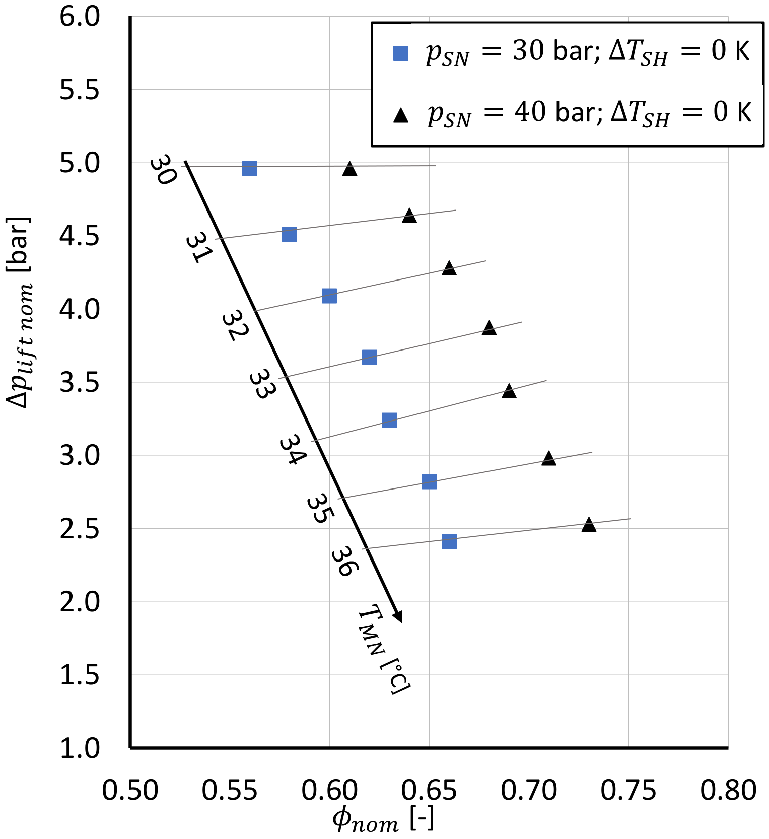
The ejector performance was estimated on the basis of the data supplied by the manufacturer and an extrapolation map, relying on experimental data.

The nominal working point, expressed in terms of the entrainment ratio ${\varphi }_{nom}$ and pressure lift $\Delta p_{lift nom}$ given by the manufacturer as a function of the motive nozzle and the suction nozzle, stated:

$${\varphi }_{nom}=\varphi \left(p_{MN}, T_{MN},p_{SN},T_{SN}\right)$$

(24)

$$\Delta p_{lift nom}= \Delta p_{lift}\left(p_{MN}, T_{MN},p_{SN},T_{SN}\right)$$

(25)

where the pressure lift was defined as:

$$\Delta p_{lift}=p_{DIFF}-p_{SN}$$

(26)

An example of the nominal performance working points of the ejector is reported in Figure 7, for a motive nozzle pressure of 90 bar.

In order to extend the numerical model to non-nominal conditions, the polynomial mode proposed by Banasiak et al., 2015 [30] was used as a reference. In this paper, a complete polynomial model of an ejector geometry named VEJ1 was developed based on an extensive experimental database. Rearranging the formulation proposed, the entrainment ratio was obtained as a function of the motive and suction thermodynamic condition and of the pressure lift:

$${\varphi }_{VEJ1}={\varphi }_{Ej1}\left(p_{MN}, T_{MN},p_{SN},T_{SN},\Delta p_{lift}\right)$$

(27)

Equation (28) was used in the model in order to predict the correlation between the lift and the entrainment ratio for values other than the nominal ones:

$$\varphi =\frac{{\varphi }_{nom}\left(p_{MN}, T_{MN},p_{SN},T_{SN}\right)}{{\varphi }_{Ej1}\left(p_{MN}, T_{MN},p_{SN},T_{SN},\Delta p_{lift nom}\right)}{\varphi }_{VEJ1}\left(p_{MN}, T_{MN},p_{SN},T_{SN},\Delta p_{lift}\right)$$

(28)

This extrapolation was accurate only when the equilibrium point of the system was close to the nominal point, and decreased as the actual working condition differed from the nominal. This will be discussed in the Results and Validation session.

Given the entrainment ratio from Equation (28) and the motive mass flow rate, the suction nozzle mass flow rate was given by Equation (29). The mass flow rate and specific enthalpy at the diffuser were given by Equations (30) and (31), which enforce the conservation of the mass and the energy:

$${\dot{m}}_{SN}=\varphi {\dot{m}}_{MN}$$

(29)

$${\dot{m}}_{DIFF}=\left(1+\varphi \right) {\dot{m}}_{MN}$$

(30)

$$h_{DIFF}=\frac{h_{MN}+\varphi h_{SN}}{1+\varphi }$$

(31)

3.6. Boundary Conditions and Control Systems

Due to the model being a dynamic one, each boundary condition had to be stated as a function of time. For stationary tests, inputs were maintained as constants. The required inputs were the water inlet conditions on both high and low pressure sides, the air inlet conditions at the finned coil heat exchanger, the compressors’ status (ON/OFF and, in case, the inverter status), and the mass flow circulating in the natural circulation flooded evaporator.

In the validation phase, these inputs were set according to the corresponding experimental values.

3.7. Solver

To evaluate the numerical solution, the software Simcenter AMESim employed a default optimized solver, based on an optimized variable integration method. When the numerical solution was evaluated, to examine its accuracy, a tolerance equal to $tol={10}^{-7}$ was chosen; after each computation step, the software integrator checked for the convergence and estimated the error: for each state, variable $y_i$, the error must satisfy the conditions ${\epsilon }_i<tol\left(1+y_i\right)$. When the iterations converged, an error test was applied to determine if the results were accurate enough, however if either of these tests failed, the integration step was replaced with a smaller step size.

4. Results and Validation

The numerical model was intended to investigate the thermal performance of the refrigerating system operating according to heat pump configuration and chiller configuration and to extend the results coming from the experimental campaign. In order to obtain the model validation, the results obtained from the model were compared against experimental data.

4.1. Validation of the Heat Pump Configuration

The validation of the numerical model was provided in both steady state and transient operation. The inputs given to the numerical model were the state of the air and the water, which were collected experimentally during the test, which were ${\dot{m}}_{air}^{IN}=25.2{ \mathrm{kgs}}^{-1}$, $T_{air}^{IN}=8.7 °\mathrm{C}$, ${\phi }_{air}^{IN}=67 \%$ for the air and ${\dot{m}}_{water,1}=2{ \mathrm{kgs}}^{-1}$, $T_{water,1}=23.9 °\mathrm{C}$ for the water.

During the steady state operation, the numerical model demonstrated good agreement with the experimental data (Figure 8), while the comparison between the main heat flow rates of the system is reported in

Table 7. Comparison between experimental data and simulation results, heat pump configuration.

Name	Variable	UNIT	EXP	NUM
Gas-cooler(1) heat flow rate	${\dot{Q}}_{g{c}_{\left(1\right)}}$	kW	169.3	169.3
IHX heat flow rate	${\dot{Q}}_{IHX}$	kW	10.1	9.6
Compressors electric power input	$P_{el,comp}$	kW	49.4	45.8
Low pressure receiver operation pressure	${\overline{p}}_{LPR}$	bar	34.5	34.4
Gas-cooler(1) water outlet temperature	$T_{water}^{OUT}$	°C	43.2	44.2
Coefficient of performance	COP	-	3.3	3.7

.

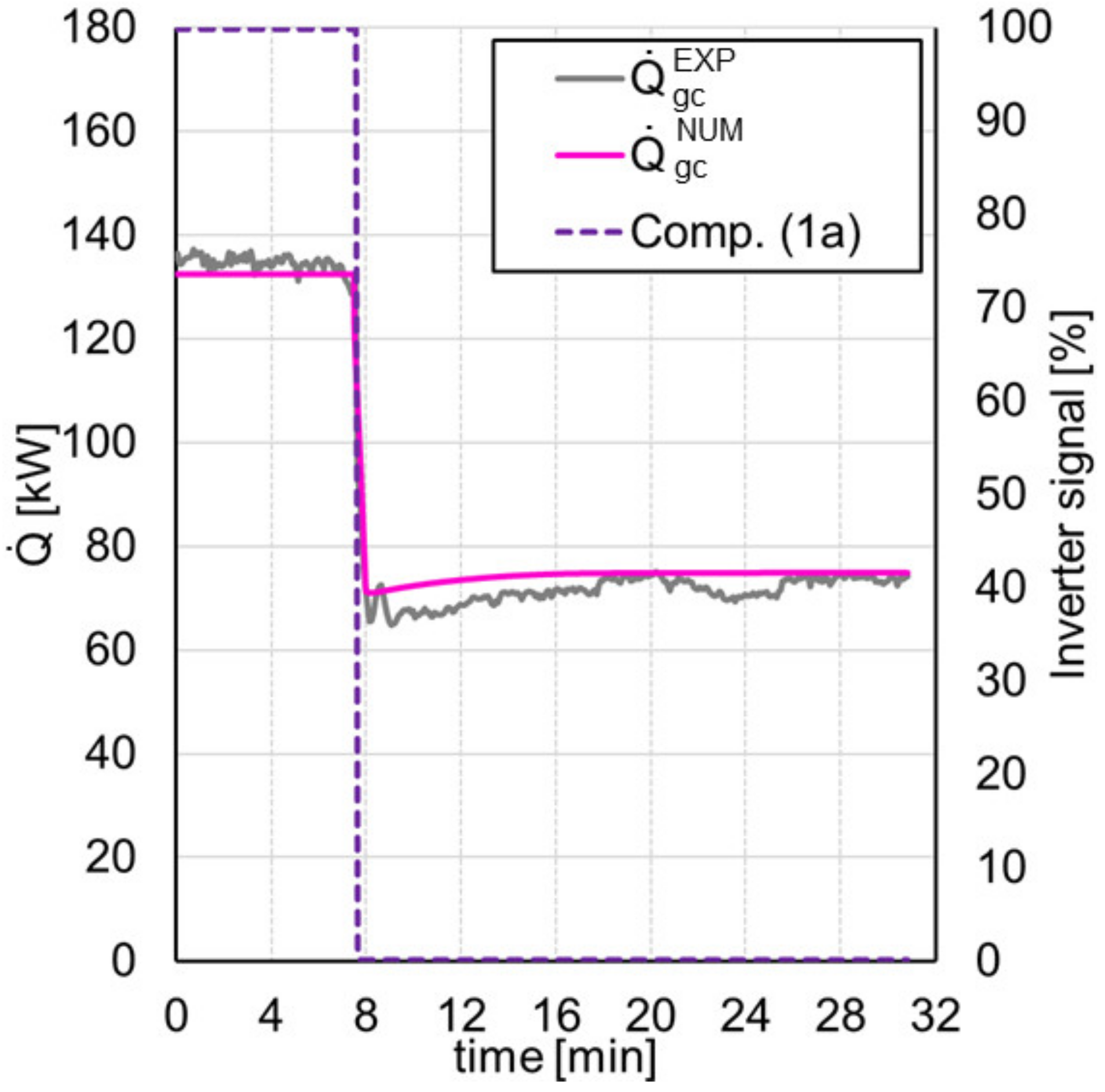
The numerical validation in transient conditions (Figure 8) was obtained by suddenly shutting down the compressor (1a) (7.5 min) after the system had previously reached steady state operating condition. Figure 9 reports the trend of ${\dot{Q}}_{g{c}_{\left(1\right)}}$ as a function of time during the steady state condition prior to the compressor shutdown, the transient evolution (7.5–24.5 min), and the following steady state operation (24.5–30 min).

The thermodynamic response of the model was found to be in accordance with the experimental data.

The difference between the experimental and numerical compressor power input was consistent with the data previously presented in Figure 5b, regarding the compressors’ characterization. The compressor nominal power consumption has been proven to be in fact 5% to 10% lower than the experimental, leading in this case to an underestimation of power input and consequent and consistent overestimation of the COP.

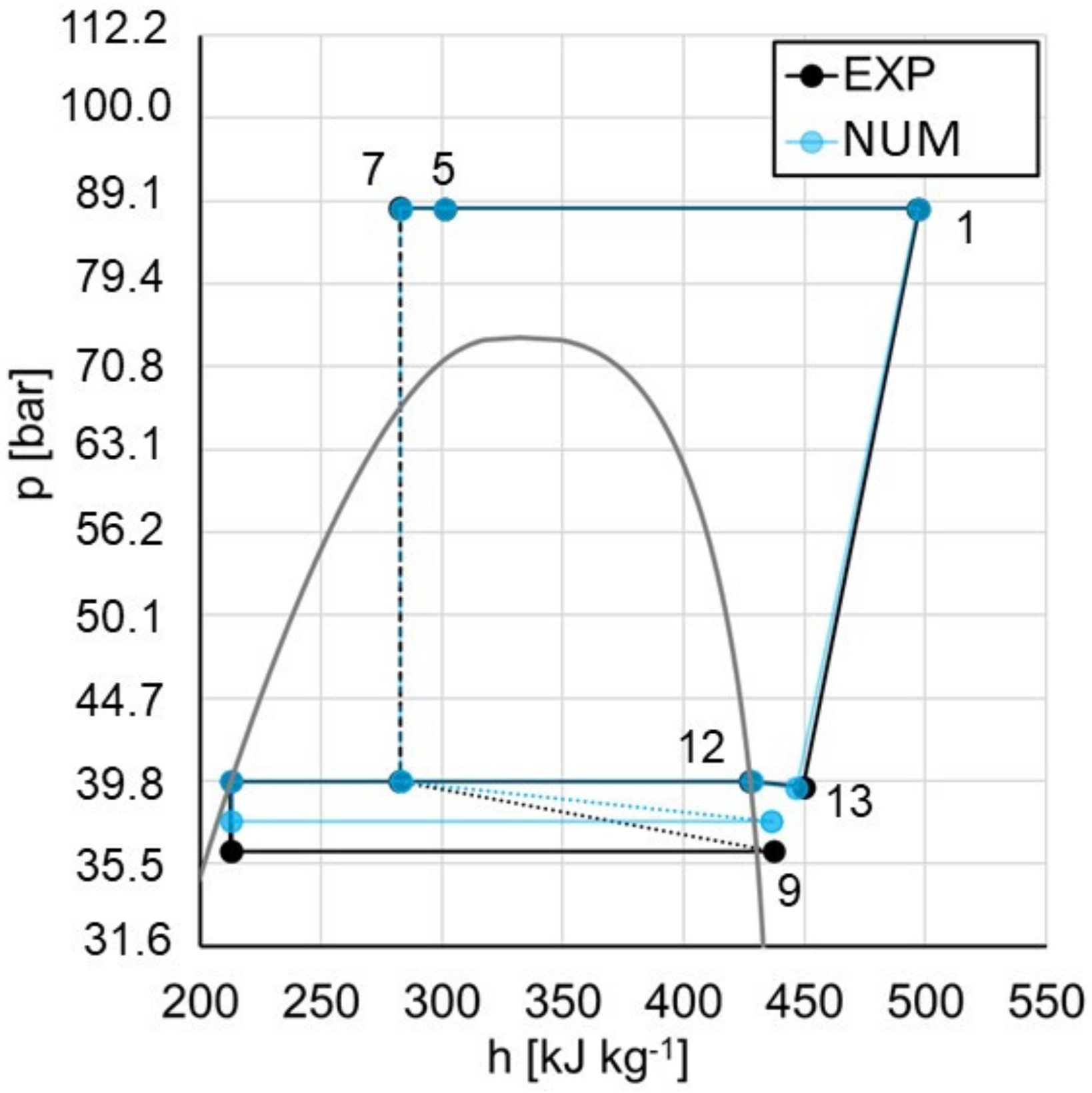
4.2. Preliminary Results in Chiller Configuration

The validation of the numerical model of the refrigerating system operating according to the chiller configuration is discussed here presenting two different cases. In both cases the system runs with a single compressor and a single evaporator: in the first one, the hot water production at the brazed plate gas-cooler is taking place while in the second one it is not.

Differently from the heat pump configuration, where each component of the system was validated ensuring a satisfying accuracy of the numerical model, in the chiller configuration, the model accuracy will depend strongly on the accuracy of the numerical model of the multi-phase ejector.

When the brazed plate gas-cooler is bypassed, the input are given by $T_{air}^{IN}=34.8 °\mathrm{C}$, ${\phi }_{air}^{IN}=84 \%$ for the air side and ${\dot{m}}_{water}=2.4 {\mathrm{kgs}}^{-1}$, $T_{water}^{IN}=12.3 °\mathrm{C}$ for the water side at the evaporator.

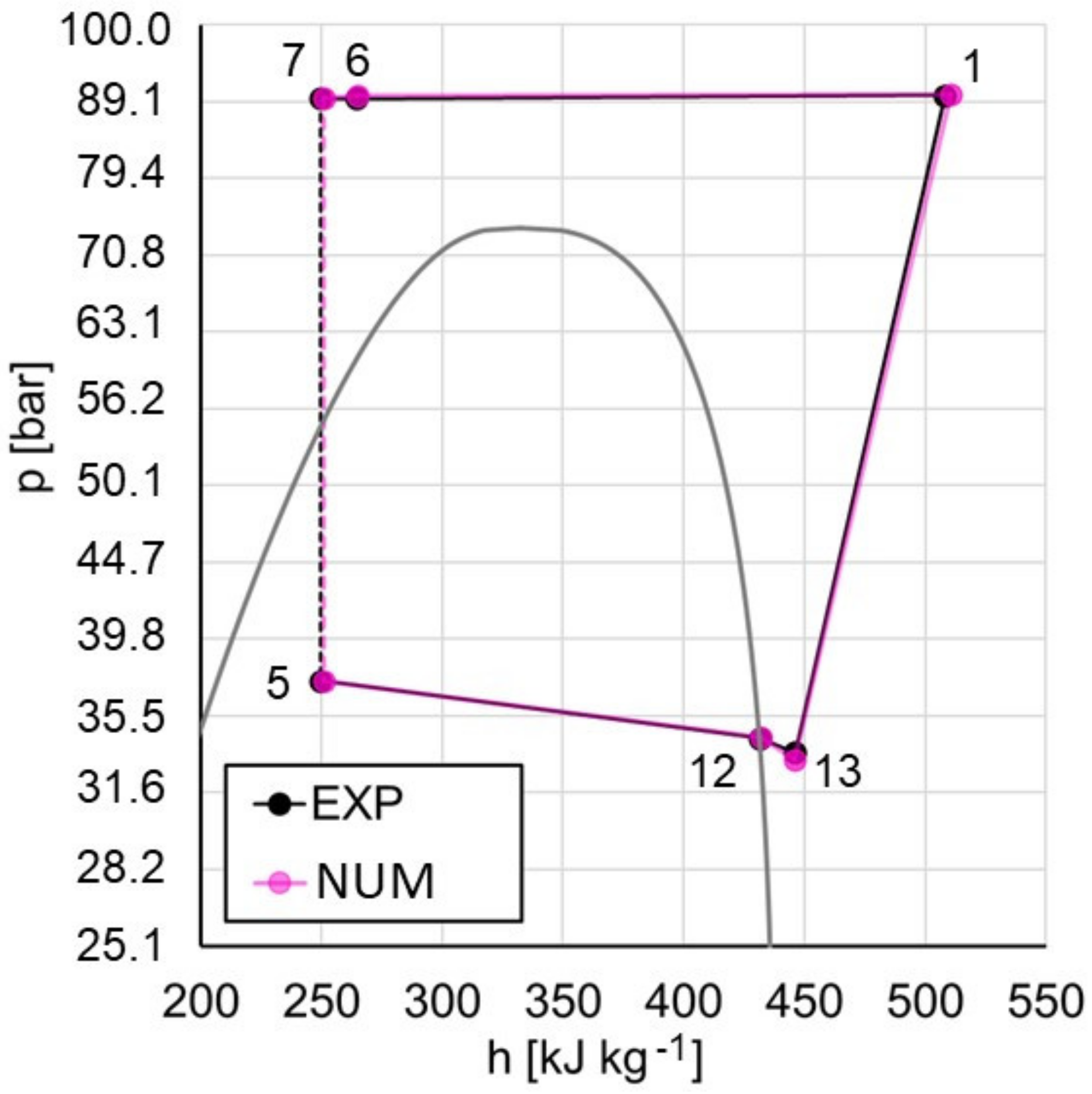
Experimental data were used to critically discuss the thermodynamic cycle (Figure 9), the energy flows of the system (Electrical power and heat flows), as well as the operating point of the ejector (

Table 8. Comparison between experimental data and simulation results, chiller configuration, brazed-plate gas cooler bypassed.

Name	Variable	UNIT	EXP	NUM
Gas-cooler(3) heat flow rate	${\dot{Q}}_{g{c}_{\left(3\right)}}$	kW	79.8	81.4
IHX heat flow rate	${\dot{Q}}_{IHX}$	kW	7.8	7.6
Evaporator(1) heat flow rate	${\dot{Q}}_{ev{a}_{\left(1\right)}}$	kW	58.6	60.5
Low pressure heat flow	${\dot{Q}}_{LP}$	kW	60.8	60.5
Compressor electric power draw	$P_{el,comp}$	kW	22.8	21.0
Ejector’s motive nozzle inlet pressure	$p_{MN}$	bar	88.5	88.5
Ejector’s motive nozzle inlet temperature	$T_{MN}$	°C	31.3	31.3
Ejector’s suction nozzle inlet pressure	$p_{SN}$	bar	36.1	37.6
Ejector’s entrainment ratio	$\varphi$	-	0.64	0.65
Ejector’s pressure lift	$\Delta p_{lift}$	bar	3.7	2.2
Low pressure receiver operation pressure	${\overline{p}}_{LPR}$	bar	39.8	39.8
Evaporator(1) water outlet temperature	$T_{water}^{OUT}$	°C	7.1	6.2
Coefficient of performance	COP	-	2.6	2.9

). During the test, the high pressure set point value was set equal to 88.5 bar while the low-pressure receiver set point temperature was set equal to 39.8 bar.

The results of the validation point were consistent with the ones presented for the heat pump operations in the previous section. The ejector equilibrium point was predicted with reasonable accuracy in terms of the recirculation factor but with a lower pressure lift. This caused the increase in the evaporation pressure visible in Figure 10. Except for this, the model obtained a good accuracy in terms of the thermodynamic description of the cycle. The compressor’s power consumption was underestimated (in the expected range 5–10%) with respect to the measured one as already discussed previously, while the heat transfer was correctly modelled. The underestimation of the power consumption led to the COP overestimation.

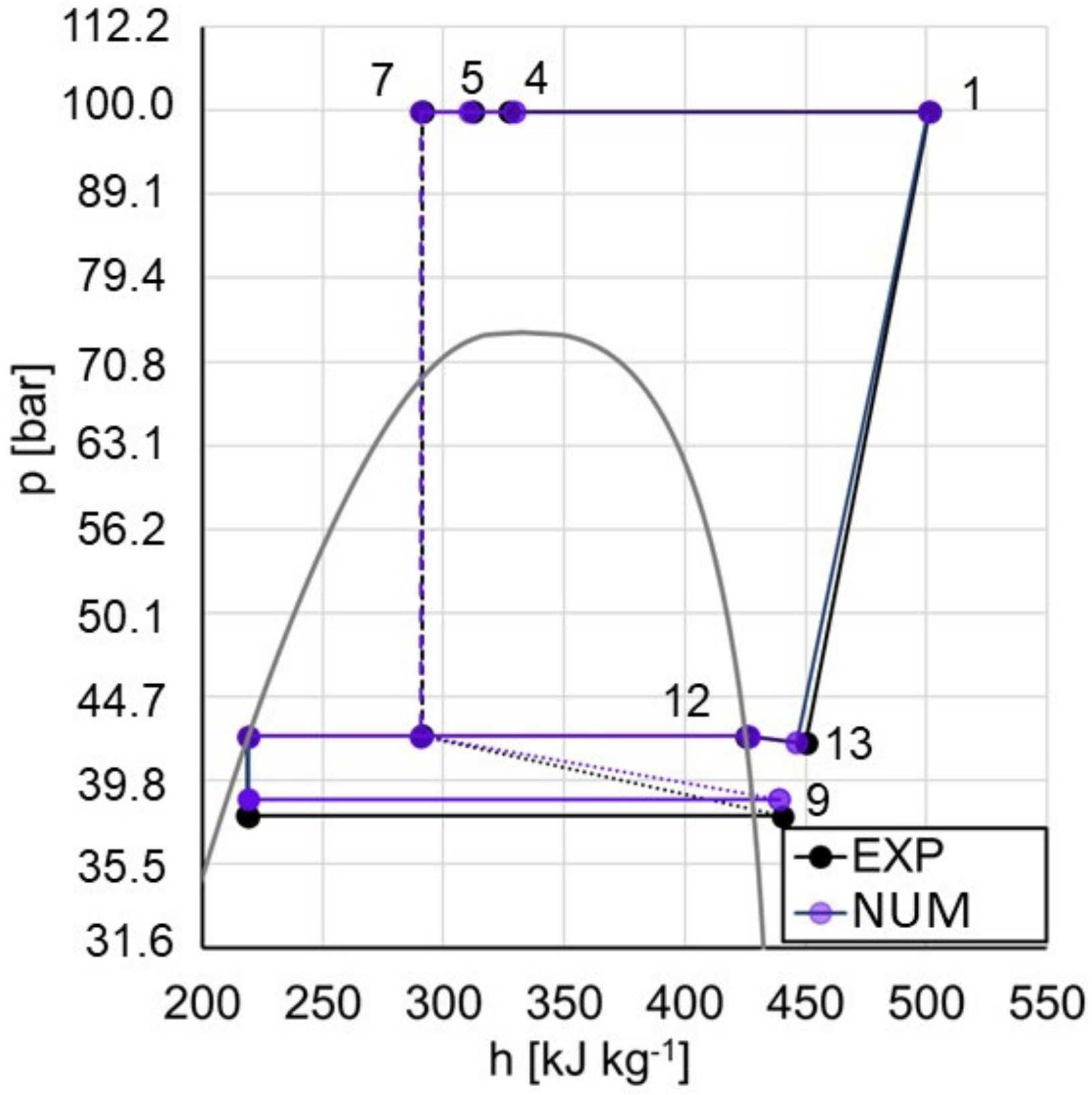
When the brazed plate heat exchanger was included (Figure 11,

Table 9. Comparison between experimental data and simulation results, chiller configuration, brazed-plate gas cooler included.

Name	Variable	UNIT	EXP	NUM
Gas-cooler(2) heat flow rate	${\dot{Q}}_{g{c}_{\left(2\right)}}$	kW	74.8	75.6
Gas-cooler(3) heat flow rate	${\dot{Q}}_{g{c}_{\left(3\right)}}$	kW	6.3	8.2
IHX heat flow rate	${\dot{Q}}_{IHX}$	kW	9.3	8.8
Evaporator(1) heat flow rate	${\dot{Q}}_{ev{a}_{\left(1\right)}}$	kW	49.9	59.8
Compressor electric power draw	$P_{el,comp}$	kW	25.6	24
Ejector’s motive nozzle inlet pressure	$p_{MN}$	bar	99.8	99.8
Ejector’s motive nozzle inlet temperature	$T_{MN}$	°C	35.2	35.2
Ejector’s suction nozzle inlet pressure	$p_{SN}$	bar	37.9	38.8
Ejector’s entrainment ratio	$\varphi$	-	0.53	0.61
Ejector’s pressure lift	$\Delta p_{lift}$	bar	4.3	3.5
Low pressure receiver operation pressure	${\overline{p}}_{LPR}$	bar	42.3	42.3
Evaporator(1) water outlet temperature	$T_{water}^{OUT}$	°C	8.8	8.1
Gas-cooler(2) water outlet temperature	$T_{water}^{OUT}$	°C	60.6	60.9
Coefficient of performance	COP	-	4.87	5.64

), the inputs to the numerical model were given by $T_{air}^{IN}=36.3 °\mathrm{C}$, ${\phi }_{air}^{IN}=84 \%$ at the finned coil gas-cooler, ${\dot{m}}_{water}=0.75 {\mathrm{kgs}}^{-1}$, $T_{water}^{IN}=36.8 °\mathrm{C}$ at the brazed-plate gas-cooler, and ${\dot{m}}_{water}=2.6 {\mathrm{kgs}}^{-1}$, $T_{water}^{IN}=13.5 °\mathrm{C}$ at the brazed plate evaporator.

In this case, the high pressure set point was set equal to 99.8 bar, while the low-pressure receiver set point operating pressure was equal to 42.3 bar.

As the water flow rate in the gas-cooler was not measured, the boundary value given to the numerical model was derived indirectly from the experimental data according to Equation (32):

$${\dot{m}}_{water}=\frac{{\dot{Q}}_{gc\left(2\right)}^{EXP}}{c_{p,water}\left(T_{water}^{OUT}-T_{water}^{IN}\right)}$$

(32)

While the high pressure side was well predicted, in this case, the evaporator heat flow was over predicted by 20%. This could be related to the ejector model, which converged for this operating point to a much higher entrainment ratio, leading to a corresponding increase in the evaporator flow rate and then heat exchange. The reported data demonstrated the high impact of the ejector model on the overall system. In contrast to the heat pump configuration, the chiller configuration cannot be considered validated. The following session will then focus on the heat pump, while the improvement of the ejector model will be the object of further research.

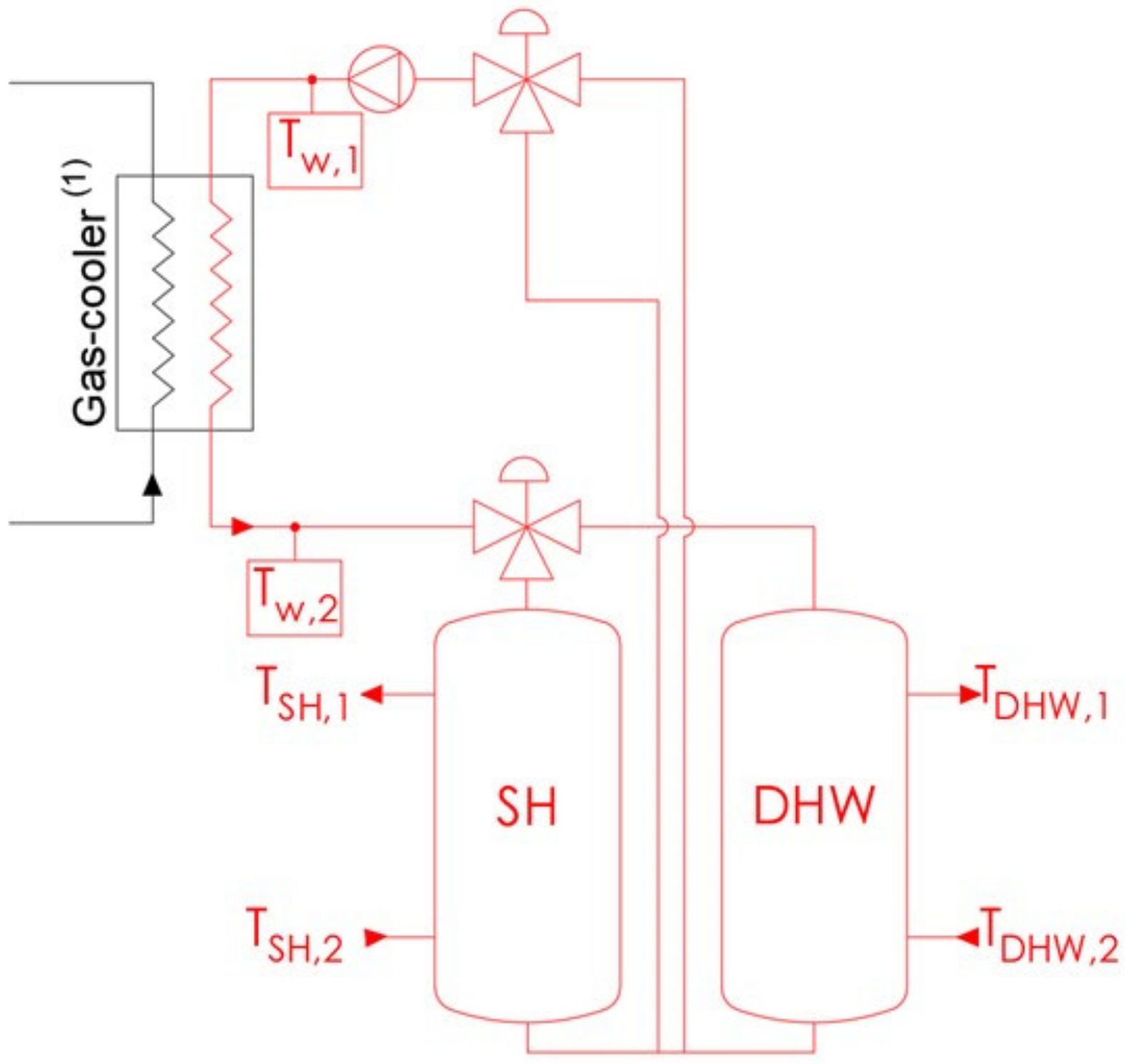
4.3. Simulation of the System Operating According to a Heat Pump Configuration

The numerical model was utilized to discuss a typical application of the refrigerating unit operating in heat pump configuration with a 24 h simulation, where the system was designed to supply heat to two different water tanks for domestic hot water (DHW) and space heating (SH), as reported in Figure 12.

The inputs into the numerical model were the state of the air at the evaporator inlet ($T_{air,IN}$, ${\phi }_{air,IN}$), assumed to be equal to the mean ambient conditions, and the hourly profile of the hot water consumption n ${\dot{Q}}_{DHW}^{load}$, ${\dot{Q}}_{SH}^{load}$ at the domestic hot water and space heating tanks, respectively.

The reference profiles for the mean ambient temperature and the thermal loads were taken from the work of Smitt et al., 2020 [31], whereas the heating demand values were scaled by a factor of 0.6, in order to adjust them to the nominal heating power of the heat pump presented in this study.

In the 24 h simulation, the water flow rate inside the gas-cooler was modulated by a PI controller in order to ensure a certain water outlet temperature depending on SH or DHW production (

Table 10. Water set-point temperature and return temperature.

Name	Variable	UNIT	DHW	SH
Water set-point temperature	$T_{water}^{set-point}$	°C	66	60
Water return temperature	$T_{water}^{return}$	°C	8	30
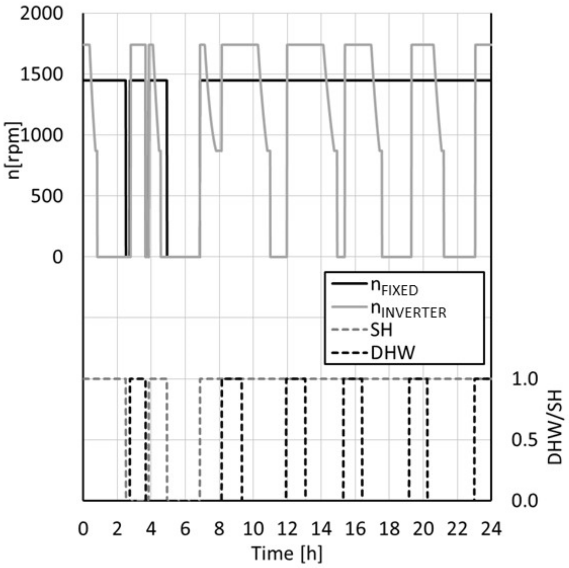
High pressure	$p_{HP}^{set-point}$	bar	105	$2.7 T_{out,gc}-6.1$

). The controller gains first guess values were obtained applying the Ziegler–Nichols method. Then slight changes were applied to obtain a good compromise between controller error and stability for the specific application. The compressors were turned on and off depending on DHW and SH demand, in particular, during DHW demand both compressors were turned on and the inverter signal was kept at 100%. However, during the SH demand the inverter signal was modulated as the DHW demand decreased, providing energy saving at the compressor.

The return water temperature boundary condition changed for SH and DHW and is reported in Table 10. As for the high-pressure control of the heat pump, during the DHW production the high-pressure was kept to a constant value of 105 bar, while during the SH production its value was evaluated depending on the refrigerant temperature at the gas-cooler outlet, according to the study of Chen and Gu., 2005 [32].

The 24 h simulation of the system was solved on a low performance notebook (AMD A8-7410 processor) in approximatively 100 s.

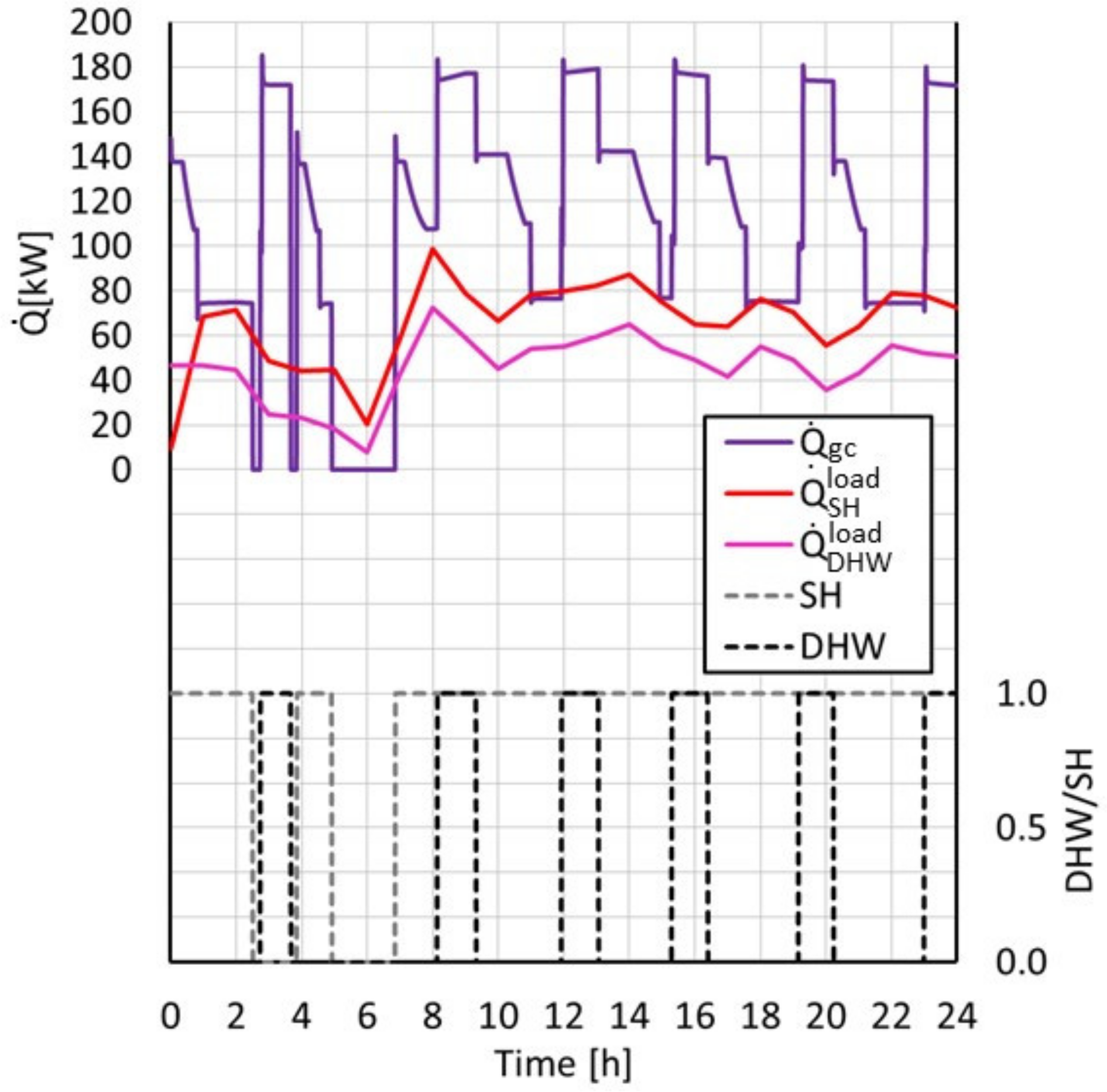
Figure 13 reports the trend of the heat flow rate provided at the gas-cooler, ${\dot{Q}}_{gc}$, as a function of simulation time and DHW/SH demand, while Figure 14 provides the trend of both compressors rotating speed as a function of the same simulation time and DHW/SH demand. It can be observed from both figures that the inverter regulated compressor modulated the rotating speed during the SH production, consequently regulating the heat flow rate at the gas-cooler and the electric power input. 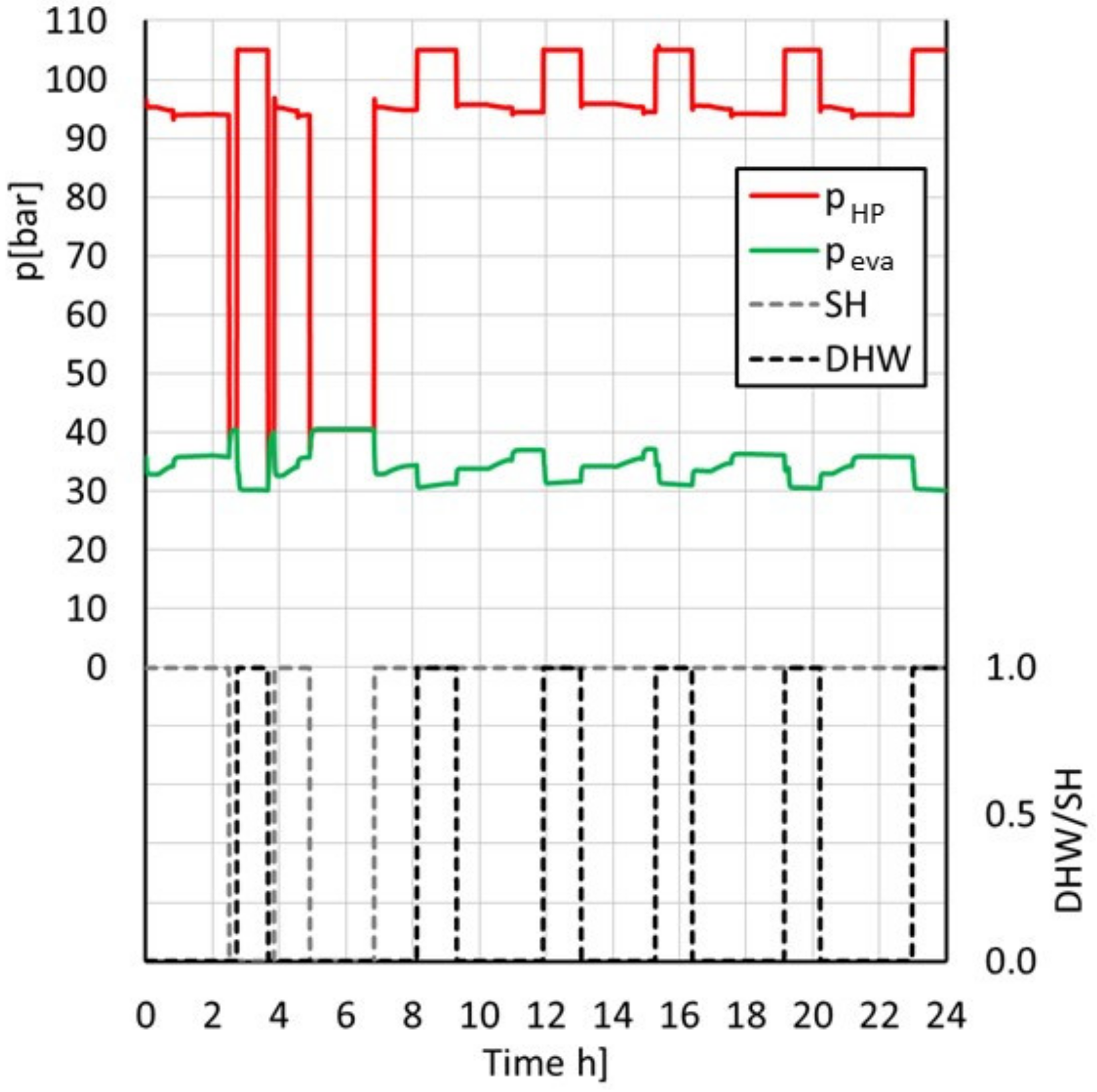On the other hand, Figure 15 reports the trend of high pressure and evaporation pressure during the simulation time. It can be observed that during the SH request time, the value of evaporation pressure stayed between 32 and 35 bar, as the high pressure was kept at approximatively 95 bar, as the refrigerant temperature at the gas-cooler outlet was at a mean value of 37.5 °C, while during DHW production the evaporation temperature was around 30 bar.

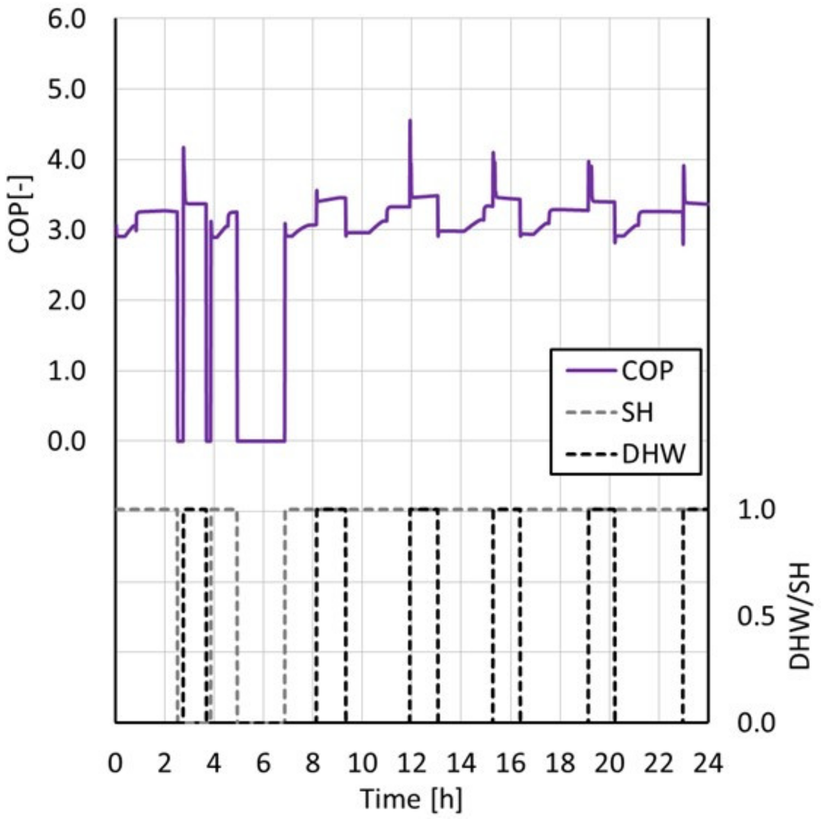
As presented in Figure 16, the numerical model demonstrated that, during DHW production, the heat pump presented a higher COP even if the mean pressure ratio between high pressure and evaporation pressure was higher than the one during SH production. The benefit is of course related to the low water temperature at the gas cooler inlet, which results in a higher useful heat flow rate at the gas-cooler. The mean values of high-pressure, evaporation pressure, water mass flow rate developed by the variable speed pump, gas-cooler heat flow rate, and COP during DHW and SH production are presented in

Table 11. Mean value of high pressure, evaporation pressure, water mass flow rate at the gas-cooler, gas-cooler heat flow rate, and COP during the simulation time.

Time [h]	Hot Water Production	${\overline{\mathit{p}}}_{\mathit{e}\mathit{v}\mathit{a}}\left[\mathit{b}\mathit{a}\mathit{r}\right]$	${\overline{\mathit{p}}}_{\mathit{H}\mathit{P}}\left[\mathit{b}\mathit{a}\mathit{r}\right]$	${\overline{\mathit{m}}}_{\mathit{w}\mathit{a}\mathit{t}\mathit{e}\mathit{r}}\left[\mathbf{k}\mathbf{g}{\mathbf{h}}^{-\mathbf{1}}\right]$	${\overline{\mathit{Q}}}_{\mathit{g}\mathit{c}}\left[\mathbf{k}\mathbf{W}\right]$	$\overline{\mathit{C}\mathit{O}\mathit{P}}$ [-]
0–2.5	SH	35.1	94.4	2627.2	91.5	3.16
2.8–3.7	DHW	30.5	105.0	2498.7	168.4	3.40
3.9–4.9	SH	34.1	94.6	3080.8	107.3	3.06
6.9–8.1	SH	33.7	95.0	3458.3	120.5	3.00
8.1–9.3	DHW	31.0	105.0	2612.0	176.0	3.43
9.3–11.9	SH	35.2	95.1	3212.6	111.9	3.12
11.9–13.1	DHW	31.7	105.0	2598.3	175.1	3.50
13.1–15.3	SH	35.0	95.5	3559.8	124.0	3.07
15.3–16.4	DHW	31.5	105.0	2538.4	171.1	3.49
16.4–19.2	SH	35.2	94.6	2798.9	97.5	3.16
19.2–20.2	DHW	31.0	105.0	2441.4	164.5	3.46
20.2–23.0	SH	35.0	94.4	2645.3	92.2	3.15
23.0–24.0	DHW	30.5	105.0	2497.7	168.3	3.31

.

5. Conclusions

This paper presented the numerical model of a CO₂ unit, which can operate according to a chiller or heat pump configuration. The numerical model was developed with the software Simcenter AMESim v.17, and its results were compared against experimental data in both heat pump and chiller configuration.

The heat pump configuration of the numerical model was validated in both steady-state and dynamic conditions. In the steady-state condition, the model was in accordance with the experimental data in operating points and gas-cooler heat flow rate. The model was also validated in dynamic conditions by suddenly shutting off one of the compressors; the model was able to correctly replicate the heat pump dynamic behaviour, with a maximum difference between the experimentally collected and predicted gas-cooler heat flow rate of 5.0%.

The numerical model assessment against experimental data was also performed in chiller configuration. The validation process demonstrated inconsistent accuracy between the two tested conditions. Furthermore, as the chiller configuration was much more complex than the heat pump one, due to the use of a flooded evaporator and two-phase ejector, further investigation is needed to provide a robust validation under different operating conditions.

Lastly, the numerical model was utilized to investigate the dynamic performance of the refrigerating system operating in heat pump configuration in a typical application where the gas-cooler was coupled with hot water tanks. The model demonstrated a higher COP when operating in DHW operations due to a higher value of gas-cooler heat flow rate.

Future work will consider:

• The validation of the numerical model of the system operating in chiller configuration in dynamic conditions and the development of a predictive model of the natural circulation evaporator;
• An experimental campaign in order to increase the accuracy of the model in the prediction of the performance of the system.
• The coupling of the system with a validated numerical model of water tanks, in order to correctly quantify the dynamic behaviour of the coupled system and discuss the optimal control strategy;
• The prediction of the system performance in a yearly simulation.
• The use of the numerical model in a theoretical study to increase the efficiency and optimize the system during operation in chiller and heat pump configuration.