2.4. Wave-Eliminating Computing Methods
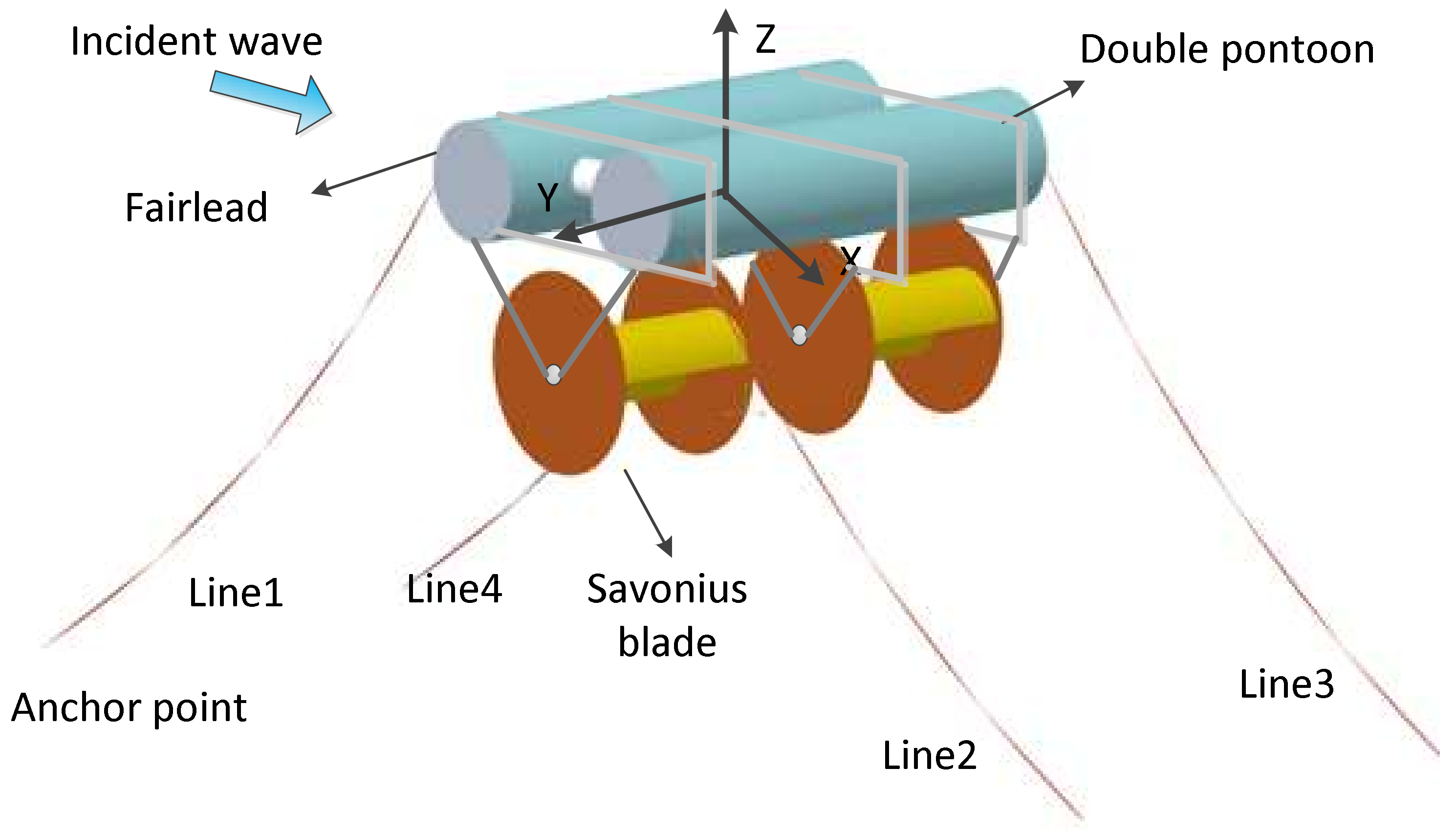
The wave velocity potential solution domain of breakwater shown in
Figure 2 can be established on the basis of the three-dimensional potential wave theory and the surface element integration method. The incident wave in the x direction passes through the diffraction on the surface of the breakwater and the radiation disturbance caused by the movement of the breakwater, and finally forms a linear superposition of the velocity potential of the three
behind the breakwater. The computational wet surfaces are divided into: free water surface
, seabed boundary
, wet surface of pontoon
, wet surface of blade
and far field boundary
. Since the Morison element
is a two-point element, its influence on the wave potential is ignored in the three-dimensional potential wave theory. Each computational wet surface should satisfy the corresponding velocity potential boundary conditions and governing equations:
The flexible breakwater makes simple harmonic motion under the action of waves, and the velocity potential of the flow field is [
10]:
where
is the incident wave velocity potential of the wave;
is the diffraction potential caused by incident waves passing through the breakwater.
is the radiation potential generated by swaying motion in still water of breakwater.
Waves will interact with ocean structures and will vibrate to a certain extent. Therefore, when choosing a turbulence model, choose the RNG model. It is a mathematical method using the renormalization group and can be derived from the Navier Stokes equation It is concluded that due to the influence of the rotation of the blade and the size of the blade, the calculation mainly focuses on the turbulence that occurs in most of the flexible breakwater and the blade under the action of waves. Therefore, using STAR-CCM+ software for numerical simulation, choose RNG k-e model for research in the physical model. Equation (3) is dissipation rate of RNG model
[
11]:
where
is the turbulent viscosity,
is the empirical parameters,
k and
are two unknown parameters, the transport equation of RNG can be expressed as follows:
By setting the physical model, grid model and solver of the flexible breakwater, it is mainly to calculate the position of the free liquid surface at the initial moment, the distribution of the velocity field, the initial velocity and damping of the blade, etc.
Through studying the state of flexible breakwaters and blades under the motion response of regular waves, the initial conditions generally do not affect the wave propagation and the calculation results after the blade motion is stabilized, but there will be certain fluctuations in the initial calculation results and subsequent results influence, the Equation (5) is the situation when
t = 0.
Since blade rotation is a planar motion relative to the breakwater coordinate system,
k only represents the three degrees of freedom of the blade. Therefore, the solution of the radiation potential of breakwater
can be obtained as follows by solving the three modes and the substituting the conditional expression (5) into Equation (2):
According to the above, the total wave velocity potential around the breakwater under linear regular waves is finally obtained. Next, the wave surface equations at each point around the breakwater are derived from the velocity potential function. The wave height data of each point, including the wave height data of the transmitted waves, represented by Ht, and the wave height data of the reflected waves, represented by Hf, are obtained from the wave surface equations. In this paper, the transmission coefficient was used to analyze the wave-attenuating performance of the breakwater.
2.5. Numerical Wave Elimination Solving Method
The purpose of numerical wave elimination is to reduce the influence of reflected waves on wave height data collection. This order value simulation uses the method of damping wave elimination. The fifth-order Stokes wave is generated at the velocity entrance of the numerical water tank and propagates to the left to the exit of the water tank.
In order to eliminate the reflected waves in the numerical simulation calculation process, it is necessary to add a damping term in the outlet fluid domain of the numerical water tank, and set the numerical wave elimination zone near the outlet boundary and away from the flexible breakwater. The setting area at the outlet is generally 1–2 wavelength distance. The formula of the damping term used to absorb the energy of the transmitted wave in the numerical wave elimination area is shown below:
where
is the relaxation function related to space coordinates, using to eliminate transmitted waves passing through the flexible breakwater,
is the velocity vector before the wave enters the wave-eliminating zone,
is The pressure field before the wave enters the wave-eliminating zone,
is the velocity vector of the wave after passing through the wave-eliminating zone,
is the pressure field after the wave passes through the wave-eliminating zone.
where
is the volume fraction of p-phase fluid in the domain cell grid,
is density of p-phase fluid in the domain,
is velocity vector of p-phase fluid in the domain.
In the process of numerical iterative calculation, the volume fraction of the two-phase fluid in the computational domain grid is further calculated based on the result of the numerical iterative calculation in the previous step.:
where
is calculation time step,
is the face value of p-phase fluid volume fraction,
is the cell volume of computational domain grid,
is volumetric flow rate of the grid area.
The radiation force is converted into a delay function by the convolution integral, and the equation used to solve the hydrodynamic time domain of the breakwater (1–16) can finally be obtained. In this equation,
:
The correction of the S-shaped blade exists in stiffness matrix
C and delay function
K. The additional radiation damping from the rotating modes of the blade
Drot is calculated using the damping formula (10), which represents the radiation damping of the rotational motion
K of the blade generated on the
jth degree of freedom of the rigid body of the breakwater; meanwhile, blade rotation changes the hydrostatic stiffness of the breakwater system, so the hydrodynamic calculation can be approximated by the modified stiffness
Krot, as shown in Equation (11) [
11].
Finally, the dynamic equation is solved through the iterative calculation by means of the Newmark-
β time-advancement scheme. It can be obtained from the micro-wave as follows:
where
K is wave number,
is the circular frequency,
H is the wave height at coordinate
x,
g is the acceleration of gravity,
d is the water depth,
T is the wave cycle,
L is the wavelength.
2.6. Solving Method for Mooring Load
The mooring system usually uses a divergent multi-chain mooring system with distributed symmetry, which can ensure the stability of the flexible breakwater and the safety of the flexible breakwater. When the flexible breakwater is in the middle position of the anchor chain distribution, the restoring force of the entire mooring system is zero, and the force received by each anchor chain is called pretension.
As shown in
Figure 3 the mooring line is divided into
N elements. In order to facilitate the calculation of the force analysis of the system and simplify the structure, it is assumed that each anchor chain in the entire anchoring positioning system converges at one point. The following formula can be derived by the geometric relationship:
where
is the suspended length of the cable chain after the floating body is offset,
is cable and chain horizontal distance after floating body offset,
is hanging length of anchor chain during pretensioning,
is transverse distance during anchor chain pre-tensioning,
is deviation angle of system.
According to the obtained horizontal component force
Q of the anchor chain, the horizontal restoring force
R of the entire system is obtained by the method of vector summation:
After the floating body is offset, the direction angle of the anchor chain changes as follows: [
12]:
is the direction angle of the anchor chain, is the horizontal component of anchor chain, is the horizontal resilience of the entire system,
2.7. Finite Element Analysis of Breakwater Model
The physical model settings mainly include the following points: selecting the fifth-order Stokes wave and three-dimensional model in the VOF wave and using Eulerian multiphase flow in the turbulence model to calculate the volume distribution of air and water, and calculate the blade position by iterative calculation. In the six-degree-of-freedom motion model, the free surface function obtains the value of the set function according to the set monitoring point.
Grid division is very important for the discrete calculation of the computer. The overlapping grid technology used in this article divides the entire computational basin into a random grid part and a background grid part. The background grid divides the computational domain into a fixed grid according to the basic size, extension method, and expansion ratio of the grid parameters. The body grid is in motion, and it moves with the flexible breakwater and Savonius-type blades without deformation, and is connected to the background grid at all times to ensure that the calculation equation can be solved. In the calculation process of the fluid domain, the grids of the floating body, the blades and the grid of the watershed are overlapped together, and no new grids will be generated during the calculation process, so the processing efficiency of dynamic grids is greatly enhanced. when the Savonius-type blade has a relatively large motion range, the quality of the grid will not decrease. The setting of grid parameters mainly includes the setting of basic grid size and grid type. The mesh model of the numerical simulation in this paper chooses to use the cut volume grid generator and the prism layer grid generator.
In order to ensure the accuracy of the calculation results of the fluid domain and the flatness of the liquid surface waves, mesh refinement is performed within the range where the free liquid surface can fluctuate and near the rotation domain of the Savonius blade. Generally, three to four are guaranteed at the dense edge. The smooth transition of the mesh of the layer can not only reduce the number of meshes, but also ensure the beauty of the mesh. The mesh gradually increases as the distance from the free liquid surface and the center of rotation of the inner blade increase. It should also be noted that the number of grids along the wave propagation direction will affect the attenuation of wave propagation energy, so the setting of specific parameters of the grid near the wave surface is also very important for numerical simulation. Close to the free liquid surface, due to the large gradient of variables such as speed and pressure, it is necessary to refine the grid in the wave height direction, which not only helps to improve the accuracy, but also facilitates the accurate capture of the free liquid surface. Meshing result
The three-dimensional (3D) grid for hydrodynamic calculation of breakwater is shown in
Figure 4 and the grid parameters in
Table 4.


