Abstract
This study presents the design and implementation of different types of manifolds (sampling system) to measure water flow properties (velocity, pressure, and temperature) through the high- and low-pressure section of a Francis-type low head hydraulic turbine (LHT of 52 m) to calculate it is efficiency using the Thermodynamic Method (TM). The design of the proposed manifolds meets the criteria established in the “International Electrotechnical Commission—60041” Standard for the application of the TM in the turbine. The design of manifolds was coupled to the turbine and tested by the Computational Fluid Dynamics (CFD) application, under the same experimental conditions that were carried out in a power plant, without the need for on-site measurements. CFD analyses were performed at different operating conditions of volumetric flow (between values of 89.67 m3/s and 35.68 m3/s) at the inlet of turbine. The mechanical power obtained and the efficiency calculated from the numerical simulations were compared with the experimental measurements by employing the Gibson Method (GM) on the same LTH. The design and testing of manifolds for high- and low-pressure sections in a low head turbine allows for the constant calculation of efficiency, avoiding breaks in the generation of electrical energy, as opposed to other methods, for example, the GM. However, the simulated (TM) and experimental (GM) efficiency curves are similar; therefore, it is proposed that the design of the manifolds is applied in different geometries of low-head turbines.
1. Introduction
The “International Electrotechnical Commission—60041” (IEC—60041) Standard establishes various test development methods to determine the hydraulic performance of different hydraulic turbomachinery, such as the Reel method, Pitot tubes, and Pressure-Time (also called Gibson), among which is the Thermodynamic Method ™. According to the standard, this method allows, in a hydroelectric power station, for the measurement of flow properties extracted in the high- and low-pressure section (inlet and outlet of the turbine or pump, respectively), to calculate the hydraulic efficiency of the turbomachinery. This method is less invasive compared to others, for example, the Pressure-Time method (also called the Gibson method). The Pressure-Time method is accurate and can inexpensively perform indirect flow measurements for low head turbines. However, it could be risky due to the phenomenon used for measurement. The application of TM instead of the Gibson method aims to avoid damage in any component of the hydraulic turbine, such as the penstock, valves, or distributor. In addition, it allows for the calculation of continuous efficiency by simultaneously measuring the interest variables without stopping power energy generation.
The IEC—60041 Standard establishes that the application of TM is limited to specific hydraulic energy values greater than 1000 J/kg (heads higher than 100 m). However, under favorable conditions, the measurement interval could be extended to lower values of the specific hydraulic energy or heads lower than 100 m [1,2].
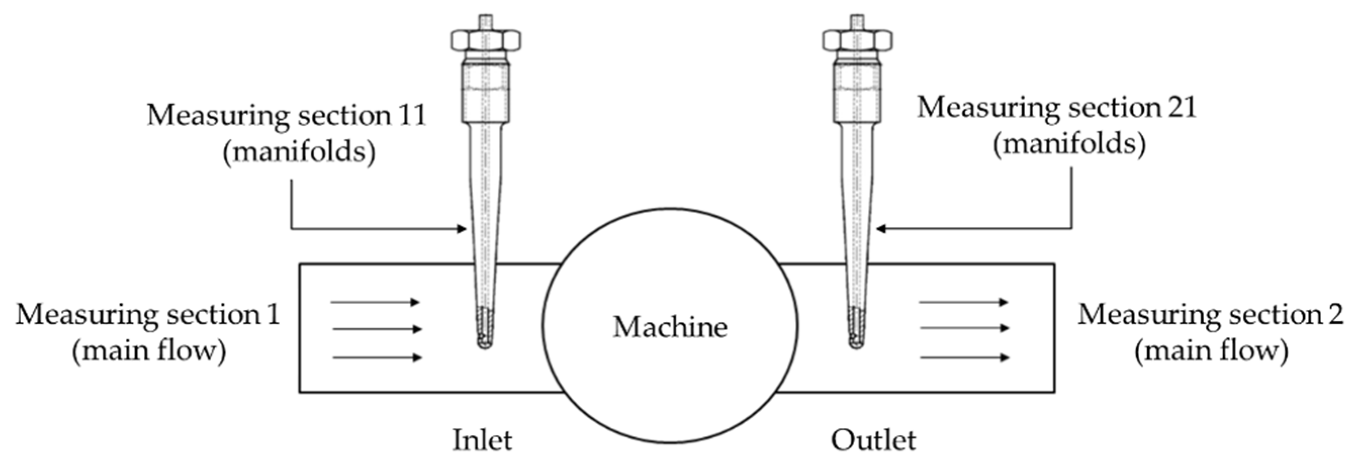
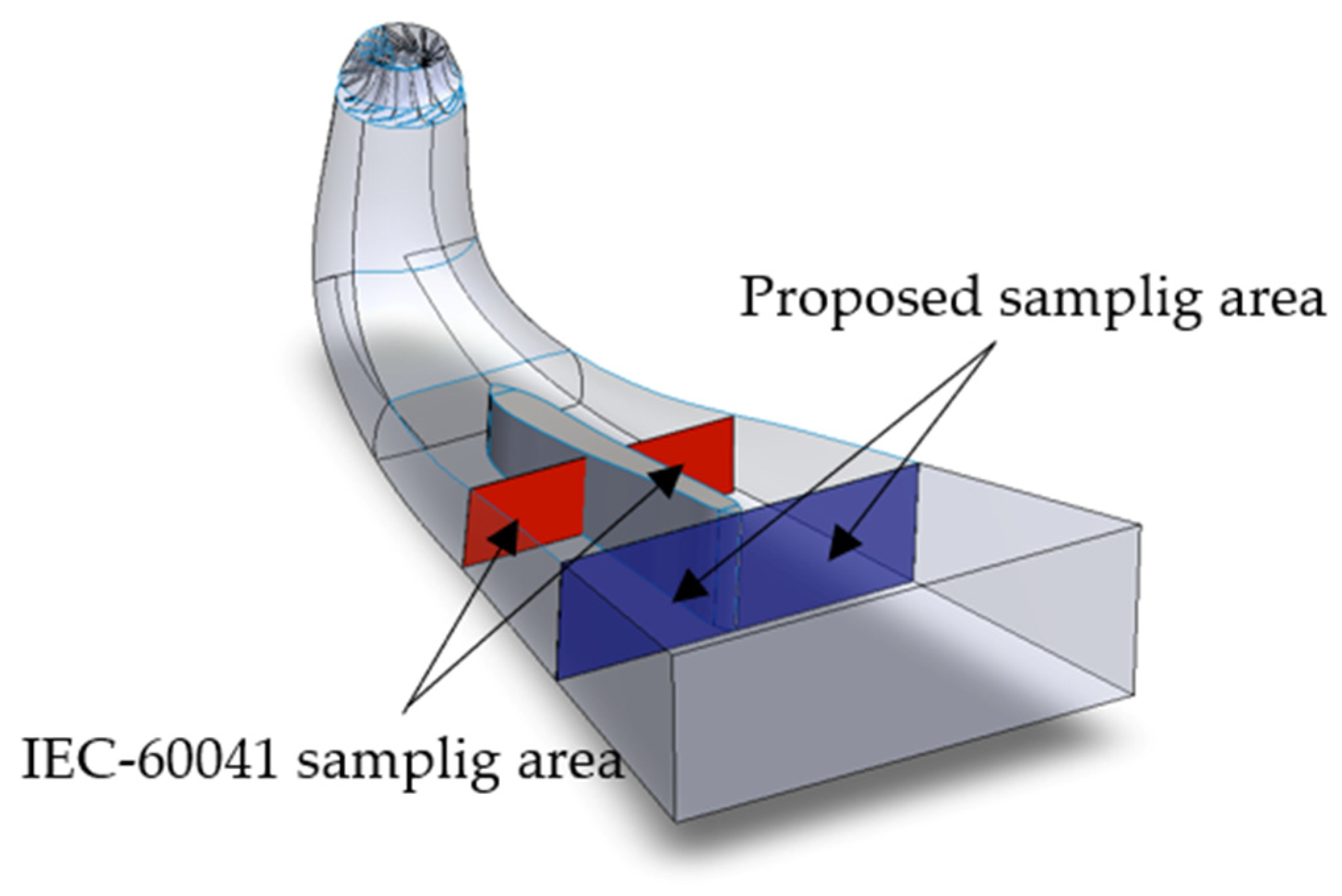
Given the inherent difficulties in directly measuring the flow that define the hydraulic efficiency (ηh), it is possible to carry out their extractions in manifolds that are especially designed for the determination of temperature, pressure, and velocity in the fluid, installing them in the inlet and outlet sections of the turbine, respectively (Figure 1).
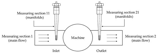
Figure 1.
Conceptual diagram showing the location of manifolds to measure flow properties to compute power and efficiency according to IEC—60041.
The manifolds must be designed to ensure that the velocity inside is at a specific interval, so that the flow is uniform when it comes into contact with the installed temperature transducers. This guarantees that the temperature will remain constant inside the manifold and around the sensor. Moreover, the precision and sensitivity of the temperature measurement instruments should be sufficient to provide an indication of a temperature difference of at least 0.001 K between the measurement points. In addition, the temperature of the extracted water should be continuously monitored by thermometers of at least ±0.05 K precision and 0.01 K sensitivity [2]. According to different authors, Pt-100 Resistive Temperature Detectors (RTD’s) are commonly used for measurement due to their high stability and precision [3,4,5].
According to TM, the direct operating procedure or direct method is used to measure the efficiency of the turbine under study. This method measures temperature, velocity, and pressure, extracting water from the penstock at the high-pressure side of the turbine to a manifold with a minimum expansion. Hydraulic losses and friction cause an increase in the temperature of the water passing through the turbine. This phenomenon can be calculated using the specific heat of the water. Although the authors of [6] defined that the decrease in the head in a turbine reduces the temperature difference between the inlet and outlet, they are directly proportional.
On the other hand, although this is a numerical case, in experimental cases, authors such as [4] propose a procedure for the normalization of experimental tests from the opening of the closing control device. After 10 min stabilization in the generator’s frequency, the temperature data recording is started by means of Pt-100 type sensors during the first 2 min. At the end, the average value of the temperature difference is calculated (high and low pressure). During this period, the measurements of the other parameters, such as inlet and outlet pressure and power, are simultaneous. This procedure is repeated for different openings of the closing control device, that is, for different load values in the unit, as in the present case.
Hydraulic turbines and the geodesic points where these are installed can present aspects of great complexity, such as installing manifolds on the low-pressure side embedded in concrete tubes. However, with a correct design of collecting tubes that are long enough for sample extraction, the measured temperature values could be considered adequate [7]. In the high-pressure section, the optimal length for penetration of the detraction into the pipe can be calculated. However, the length established by IEC-60041 could be enough [8,9,10,11].
IEC-60041 establishes that the design of detraction probes for the high-pressure zone must present the appropriate structural study to avoid total or partial detachment, and that it reaches essential areas such as the runner, causing significant damage. To select the correct materials for the probes that support the loads, the typical properties of the materials used in engineering can be consulted [10,11].
According to [3], the design of a horizontal sampling system at the outlet of the turbine is better than vertical. However, the research is based on a Pelton-type turbine. According to the turbine types, the power distribution and partial flow passage can demonstrate significant differences for the present study.
On the other hand, the system can be designed by two or more means of sampling; for example, a system composed of an arrangement of horizontal tubes with a central mixing chamber, in which the relevant sensors are coupled. Furthermore, perforated tubes are located at the turbine’s outlet, and temperature sensor is placed at different heights to measure temperature changes throughout the section.
A hybrid vertical detraction system and a mixing chamber for each tube would reduce the number of sensors required and improve measurement. In addition, the use of perforated tubes for the water samples at the outlet of the turbine omits the presence of elbows to avoid friction losses [12].
The development of accurate instruments allows for the application of TM in low head turbines; for example, most hydroelectric power plants in Mexico have heads lower than 100 m, such as 22 and 76 m. Consequently, the present study focuses on a 52-m head Francis-type hydraulic turbine installed in a hydroelectric plant in México. This has a rotational velocity of 180 RPM (18.84 rad/s) under normal operating conditions, i.e., constant volumetric input flow (between values of 89.67 m3/s and 35.68 m3/s), and a 3.5 m maximum tip diameter for the runner.
With these values, the specific speed in the turbine is calculated according to [13,14,15,16], see Equation (1). N is expressed in RPM, Q is the volumetric flow in (m3/s) and H is the head in meters.
The turbines can be classified according to the specific speed, at the head (H), a range from 50 to 240 m can be found the Francis turbine, and their specific speed is between 51 and 255 dimensionless (Power in kW) [16]. Therefore, the specific speed value for the studied turbine is 87.93, i.e., a Francis slow turbine.
On the other hand, an example comparison of the efficiency calculations in a turbine was performed using the Gibson Method (GM) and the TM at the Gråsjø power plant in Norway, which show differences between the efficiency curves below 0.5%, for the entire range measured below 0.15% and for relative powers between 0.5 and 1.15%. The Gråsjø power plant is equipped with a vertical Francis turbine and has a net height of 50 m [17], which serves as a reference for current research development.
2. Materials and Methods
2.1. Measurement System Design
2.1.1. Manifolds Design for the High-Pressure Section (Inlet)
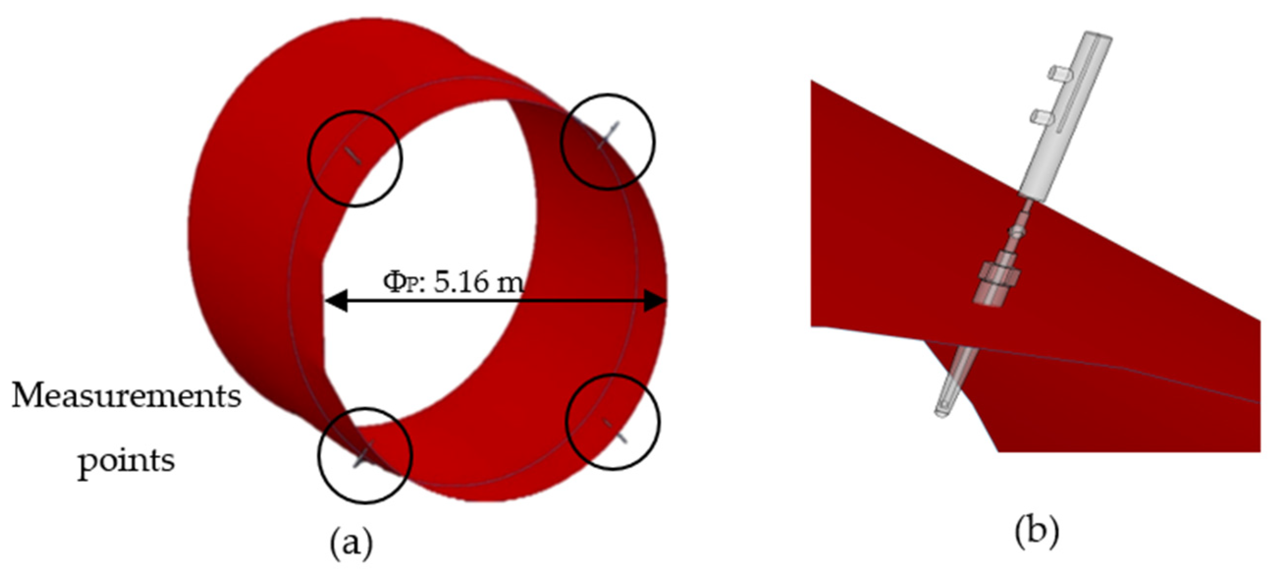
According to Castro [18] and Urquiza [19], the principal parameters were obtained to design the manifolds used in TM on the turbine´s inlet section. The values shown in Table 1 are the final results of the Gibson method, applied on a 52.54 m head turbine under different working conditions. (QT) it is the net volumetric flow, (Q0) is leakage flow when wicked gates are closed, (P1) is inlet pressure in the flow of water, (Pm) is the mechanical power energy generated by the runner, (Pe) is the electrical power measurement in the generator, (Torque) is the torque generated by the runner, (ηh) is the hydraulic efficiency of the turbine and (ηg) is the efficiency measured in the generator. The number of manifolds and their positioning is shown in Figure 2. The proposed design is shown in Figure 3 [20].

Table 1.
Parameters of the turbine on study [18,19].

Figure 2.
Measurement system, high-pressure section: (a) general view, (b) upper-right probe and manifold, zoom.
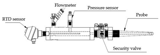
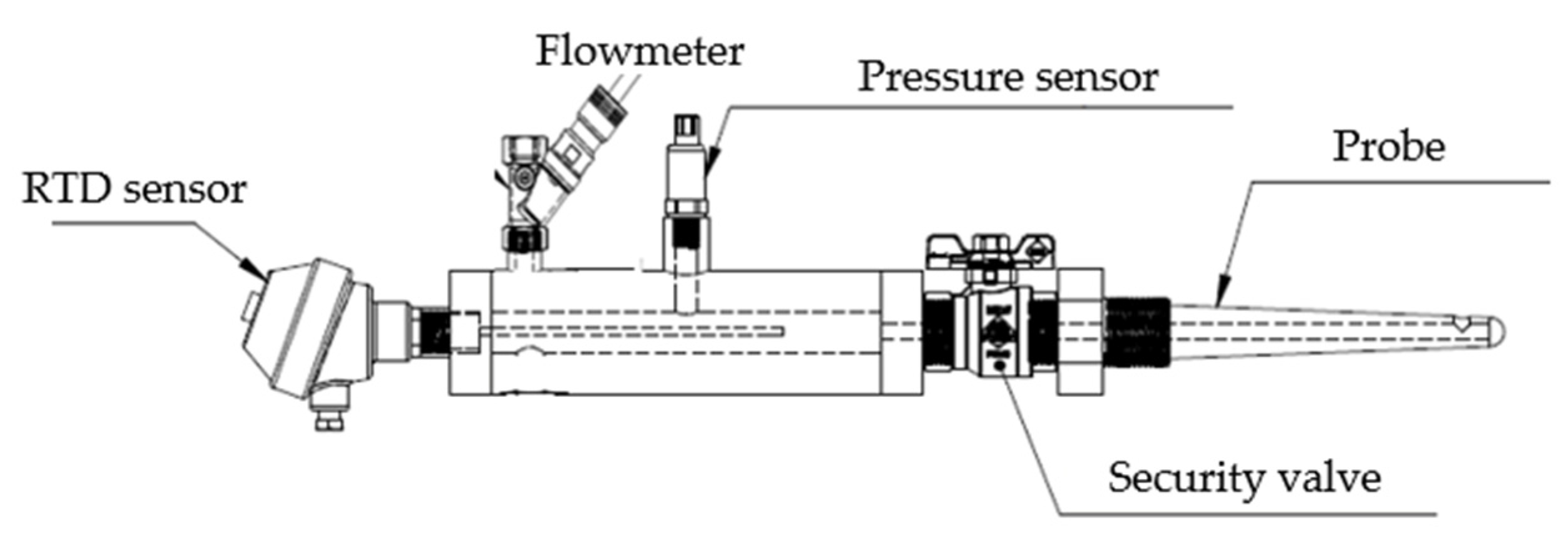
Figure 3.
Manifold proposed and instrumentation.
According to [19], for each volumetric flow, the rotational velocity is 180 RPM (18.84 rad/s), and the total deviation of measurements was ±1.6%. It is possible to define the total deviation of measurements of the flow in a systematic way, with Equation (2):
where:
- δΔρ —Uncertainty regarding the change in water density due to subsequent pressure change.
- δΔA—Uncertainty regarding the change of pipe section due to the change in pressure.
- δC—Uncertainty regarding the determination of the C-value (C = L/A).
- δρ—Uncertainty regarding the value of water density.
- δΔp—Uncertainty regarding errors in measuring pressure differences between sections of the pressure pipe.
- δΔpf—Uncertainty regarding the decrease in pressure in the section of the pipe that generates hydraulic losses.
- δt—Error relating to measurement over time.
- δQl—Relative uncertainty of measurement under final conditions by assessing flow intensification (leakage intensification).
- δrp—Error regarding the pressure change log.
The probe intrusion depth in the pressure tube for the extracted water samples is 170 mm, placed diametrically opposite to, or at 90° from, each other. According to Côté [9], the increase in the intrusion length does not represent significant changes between the results obtained with a longer probe (50 mm minimum). The differences between the results obtained with probes of different length were small, and no greater than those obtained with probes of the same length. On the other hand, the intrusion depth of the probe is at an optimum point where the main velocity produces a velocity equal to the average falling velocity of the turbine at the probe inlet. The optimal penetration where this condition is fulfilled is reported for different flow velocity profiles within the penstock [8].
However, the power of the turbine shaft (Pm) or mechanical power has been calculated with Equation (3):
where Pe is the generator active power (measured on site), ηg is the efficiency of the generator (obtained from the manufacturer), and Pf = (PtB + PgB) are the losses in the load-bearing block (PtB) and the guide-bearing (PgB). The losses have been calculated in accordance with the IEC 60041 standard.
Pm = (Pe/ηg) − Pf
2.1.2. Manifolds Design for the Low-Pressure Section (Outlet)
For the study of energy transfer in the low-pressure section, the geometry and design parameters were obtained by Castro [18]. The low-pressure section is made up of a rotating domain and a stationary one. The first is made up of the runner, hub and shroud of the turbine; the second is made up of the draft tube, divider and outlet of the section.
According to the standard, the distance of the traction intakes in this section must be located at a distance from the runner of at least five times its maximum diameter; for the turbine in question, the tip diameter of the runner is 3.5 m and the minimum distance required is 17.5 m. However, the manifolds were located farther away than the minimum distanced required to avoid turbulence generated in the walls, close to the division of the draft tube (see Figure 4).

Figure 4.
General geometry low section pressure (isometrical view).
Hulaas establishes that, under favorable conditions, the application of TM can be extended to falls of less than 100 m; on the other hand, since it is an inaccessible, closed measurement selection, the only possibility of exploring the temperature is through an intake device located inside the tube. This device consists of at least two tubes that collect partial flows [1,2].
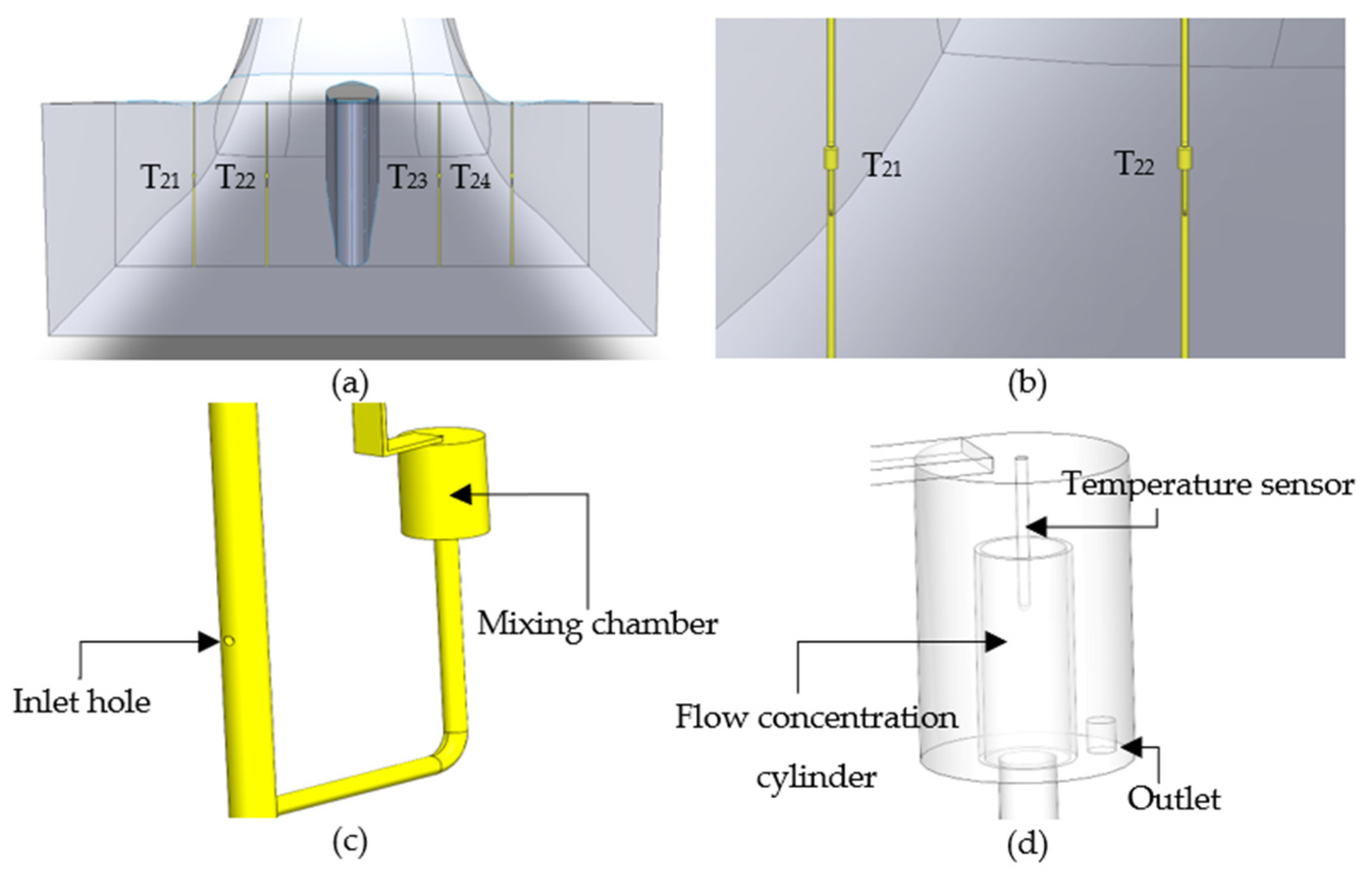
Based on Figure 4, four fluid withdrawal intakes were coupled to perform temperature, flow rate and pressure measurements at the outlet of the draft tube; the proposed design is shown in Figure 5.
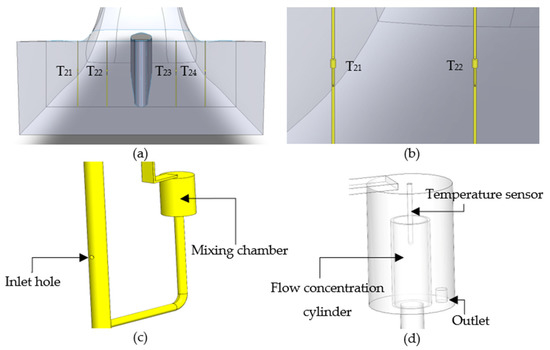
Figure 5.
Manifold vessels coupling, outlet section: (a) manifolds T21, T22, T23 and T24, (b) view outlet section left, (c) isometric view of manifold vessel, (d) mixing chamber (inside).
2.2. Numerical Simulation (CFD)
The computational fluid dynamics (CFD) analysis for the high- and low-pressure sections was performed in commercial software (ANSYS CFX). The domain discretization was performed by ICEM for both domains, and both the numerical calculation, and the post-process were performed by ANSYS CFX.
The discretization of the high-pressure section was of the non-structured tetrahedral type, presenting a total of 1,273,913 elements. In both the high- and low-pressure section, the element unit is millimeters (mm).
For the high-pressure section, the minimum size of the element is 1 mm, and the maximum size is 480 mm. This section includes the temperature sensors, probes, manifolds, inlet, outlet, and penstock.
The discretization for the low-pressure section is also that of the non-structured tetrahedral type, presenting a total of 6,297,796 elements. On the other hand, united with the elements, smaller bodies such as collector tubes (manifolds), mixing chambers, RTD’s, and the flow inlet and outlet locations are added. For the low-pressure section, the minimum size of the element is 1 mm, and the maximum size is 600 mm. This section includes the temperature sensors, manifolds, runner, inlet and outlet of turbine, and draft tube, respectively.
For each of the numerical simulations, mass flow conditions calculated from the inlet volumetric flow were established.
According to [21], some turbulence models, such as k−Epsilon, are only valid for fully developed turbulence, and do not perform well in the area close to the wall. Two ways of dealing with the near-wall region are usually proposed.
One way is to integrate the turbulence with the wall, where turbulence models are modified to enable the viscosity-affected region to be resolved with all the mesh down to the wall, including the viscous sublayer. When using a modified low-Reynolds turbulence model to solve the near-wall region, the first cell center must be placed in the viscous sublayer (preferably y+ = 1), leading to the requirement of abundant mesh cells. Thus, substantial computational resources are required.
Another way is to use the so-called wall functions, which can model the near-wall region. When using the wall functions approach, there is no need to resolve the boundary layer, causing a significant reduction in the mesh size and the computational domain. Then:
- -
- First, grid cell need to be 30 < y+ < 300. If this is too low, the model is invalid. If this is too high, the wall is not properly resolved.
- -
- The high-Re model (Standard k−Epsilon, RNG k−epsilon) can be used.
- -
- This method is used when there is greater interest in the mixing than the forces on the wall.
For the present case, the absolute distance from the wall in temperature sensors (walls of greater interest) is 0.97 mm (y), the Re number is 3998.2, the skin friction (Cf) is 0.013, the Wall shear stress (τw) is 2.44 Pa, the friction velocity (u*) is 0.049 m/s and the y+ value is 47. As the y+ value is in the range 30 < y+ < 300, both the turbulence model k-Epsilon and mesh are applicable for the study.
2.2.1. High Pressure Section
The high-pressure domain (penstock, Figure 6) was established as a stationary numerical analysis, with a k-Epsilon turbulence model and the Total Energy model to obtain temperature changes at strategic points in the domain. The fluid temperature at the inlet was 25 °C, and the walls of the study domain were defined as adiabatic.

Figure 6.
CFD, Post-processing. High-pressure section: Isometric view.
The boundary condition at the input was established as a mass flow rate and the outlet was established as a pressure outlet. Both the inlet and outlet conditions are presented in Table 1; for example, the first simulation is a development to 89,418.9 kg/s (89.67 m3/s) and 390 kPa values, respectively. A total of 2000 iterations were established, with a convergence criterion of residual type “RMS”, with a value of 1 × 10⁻⁶ and, for energy, a value of 1 × 10⁻⁴.
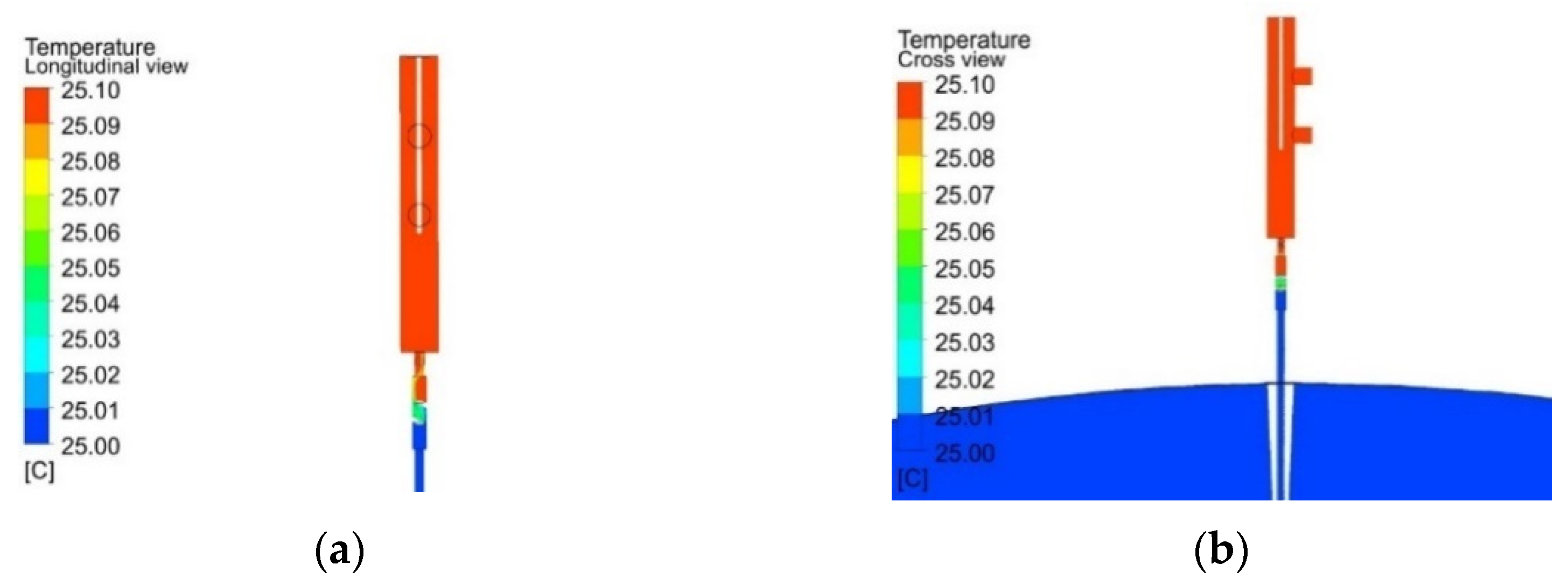
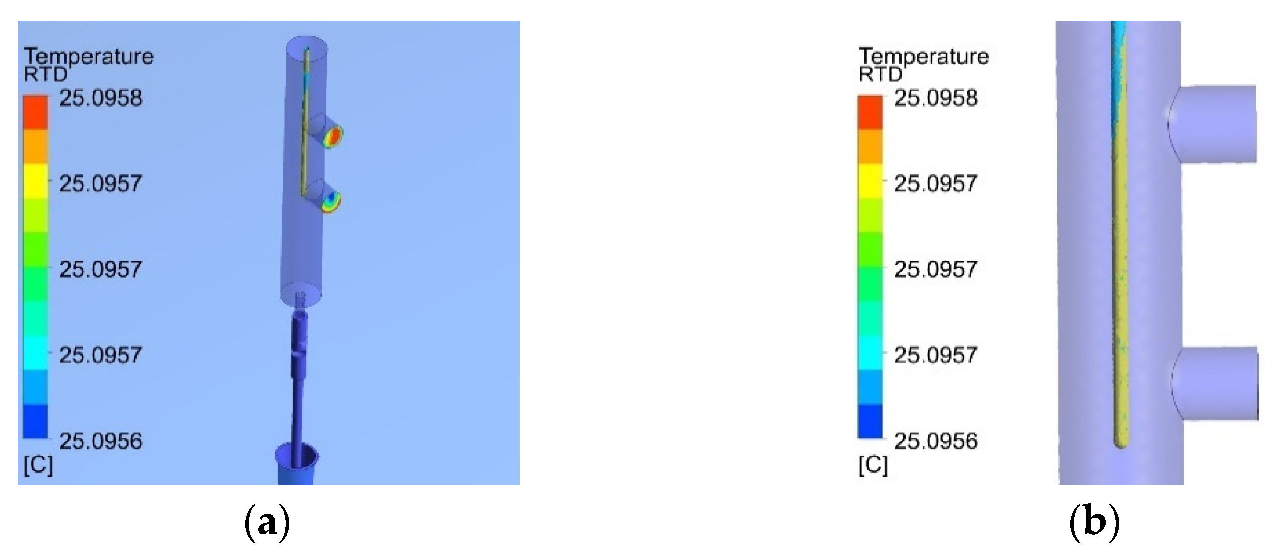
The post-processing of the interest variable in the software shows the water temperature inside the manifolds (Figure 7), and the temperature on the surface of the RTD instrument through color contours (Figure 8), in which the higher value corresponds to the red color and the minor to the blue. The RTD sensor, a simulated surface within the study domain, directly obtains the necessary resolution for temperature measurement. The dimensions of the simulated sensor are 4 mm in diameter and 152 mm long [20]. Proper mixing of the fluid is confirmed by means of the temperature contours inside the manifolds, and a constant temperature is ensured. The maximum temperature of the fluid inside the manifolds is 25.1 °C, and the maximum temperature on the surface of the RTD sensor is 25.09 °C.

Figure 7.
Internal temperature vessel, high-pressure section: (a) Longitudinal view, (b) Cross view.

Figure 8.
RTD temperature, high-pressure section: (a) Isometric view, (b) Longitudinal view (zoom).
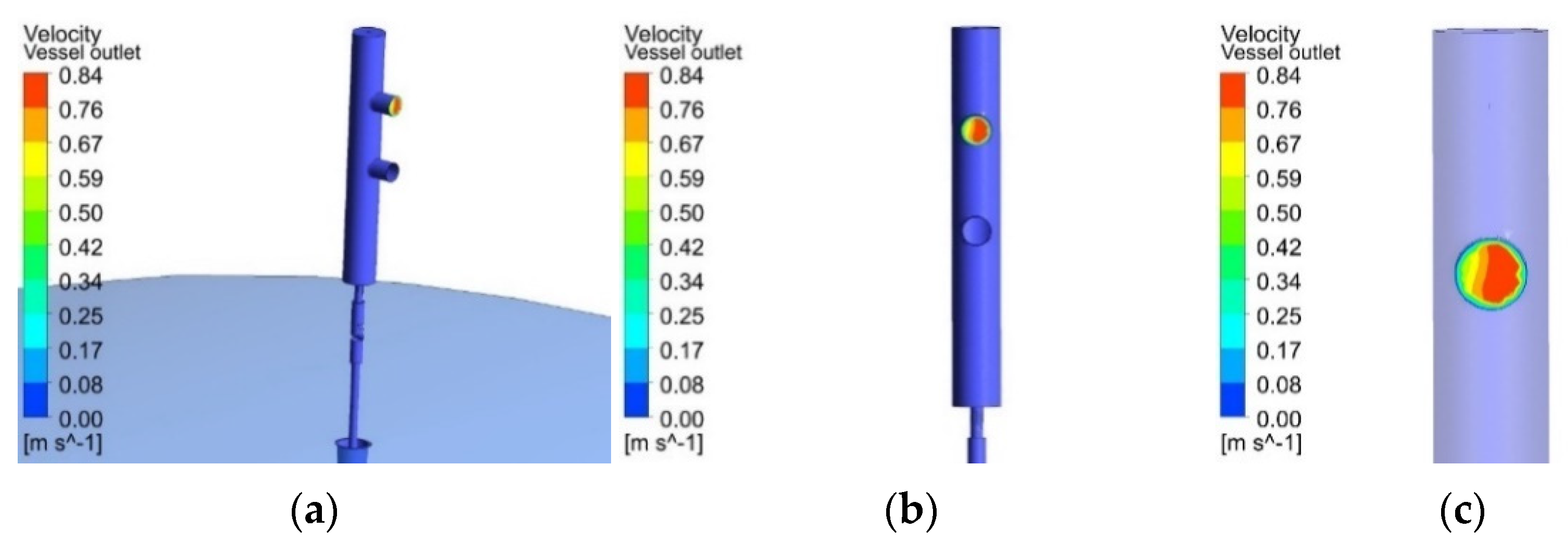
According to the standard, at the manifold outlet, the volumetric flow must be between 0.1 × 10⁻³ and 0.5 × 10⁻³ m3/s; therefore, the expected velocity range will be between 0.29 m/s and 1.46 m/s, respectively, since the outlet diameter of the manifolds is 0.02 m. Figure 9 shows the outlet velocity of the manifolds using colored contours. The obtained results confirm the values that are allowed by the standard.

Figure 9.
Velocity outlet, high-pressure section: (a) Isometric view, (b) Front view, (c) location velocity outlet (zoom).
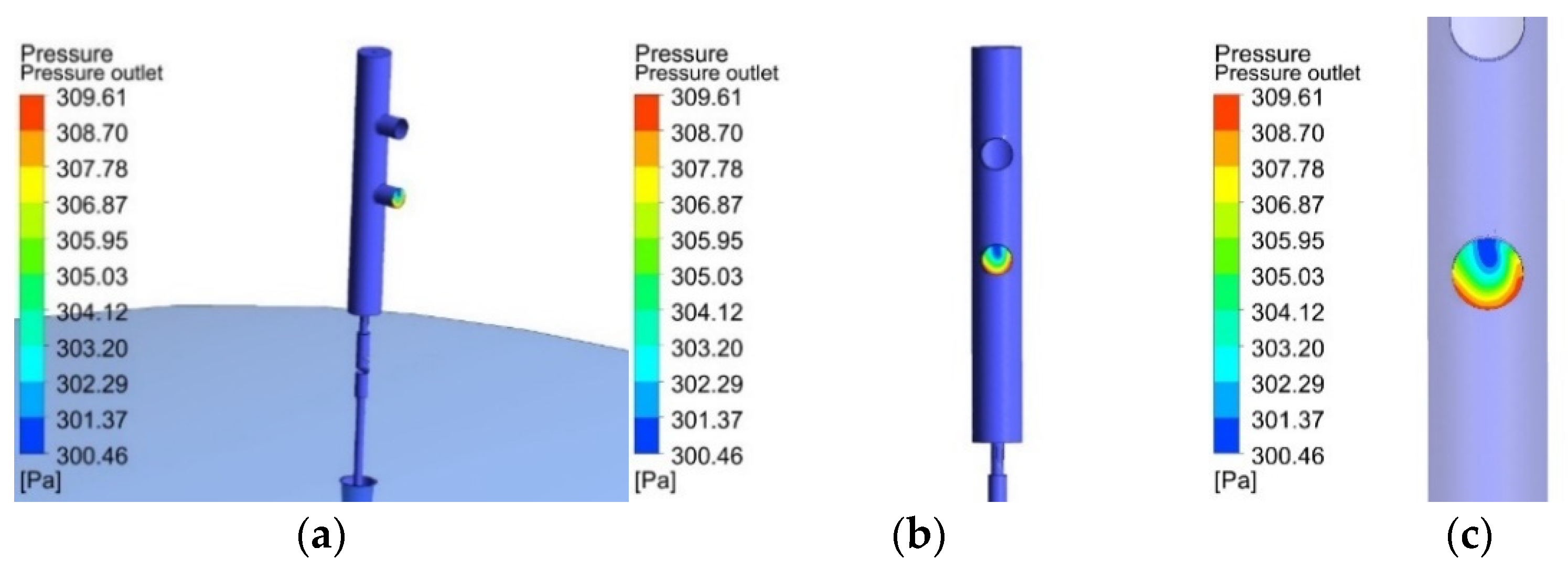
On the other hand, Figure 10 shows the pressure contours at a location where a relevant sensor is physically attached.

Figure 10.
Pressure location, high-pressure section: (a) Isometric view, (b) Front view, (c) location pressure outlet (zoom).
2.2.2. Low Pressure Section
The CFD in the low-pressure section, as well as in the high-pressure one, used different inlet mass flows (presented in Table 1); however, the pressure at the outlet of the turbine (draft tube) was established as a pressure static outlet or open to the atmosphere. The numerical simulation was of the “turbo-machinery” type, defining a rotating domain (runner) and a stationary domain (draft tube and manifolds). When using two types of domains, it is necessary to establish a new boundary condition, defined as an interface. This configures itself as a “stage” type, since it adapts the results of a domain with movement to a stationary one, in which it is determined to be a “fluid–fluid” interface with corresponding 360° angles. A volumetric flow inlet with a direction based on cylindrical components was defined, a rotational velocity of the runner at 180 rpm and the temperature of the inlet fluid was that obtained at the outlet of the penstock for each of the different cases. The k-Epsilon turbulence model and the Total Energy equation were enabled; similarly, the domain walls were adiabatic, as in the penstock. In both the low- and high-pressure section, one of the most prominent turbulence models, the (k-Epsilon) model, was used. This is implemented in most general purpose CFD codes and is considered the industry standard model. It has proven to be stable and numerically robust and has a well-established regime of predictive capability. Therefore, for general-purpose simulations, the model offers a good compromise in terms of accuracy and robustness.
Within CFX, the turbulence model uses the scalable wall-function approach to improve robustness and accuracy when the near-wall mesh is refined. The scalable wall functions enable solutions to arbitrarily fine near-wall grids, significantly improving standard wall functions. Defined thus, a total of 10,000 iterations were established with a convergence criterion of residual type “RMS” with a value of 1 × 10⁻⁶ and, for energy, a value of 1 × 10⁻⁴.
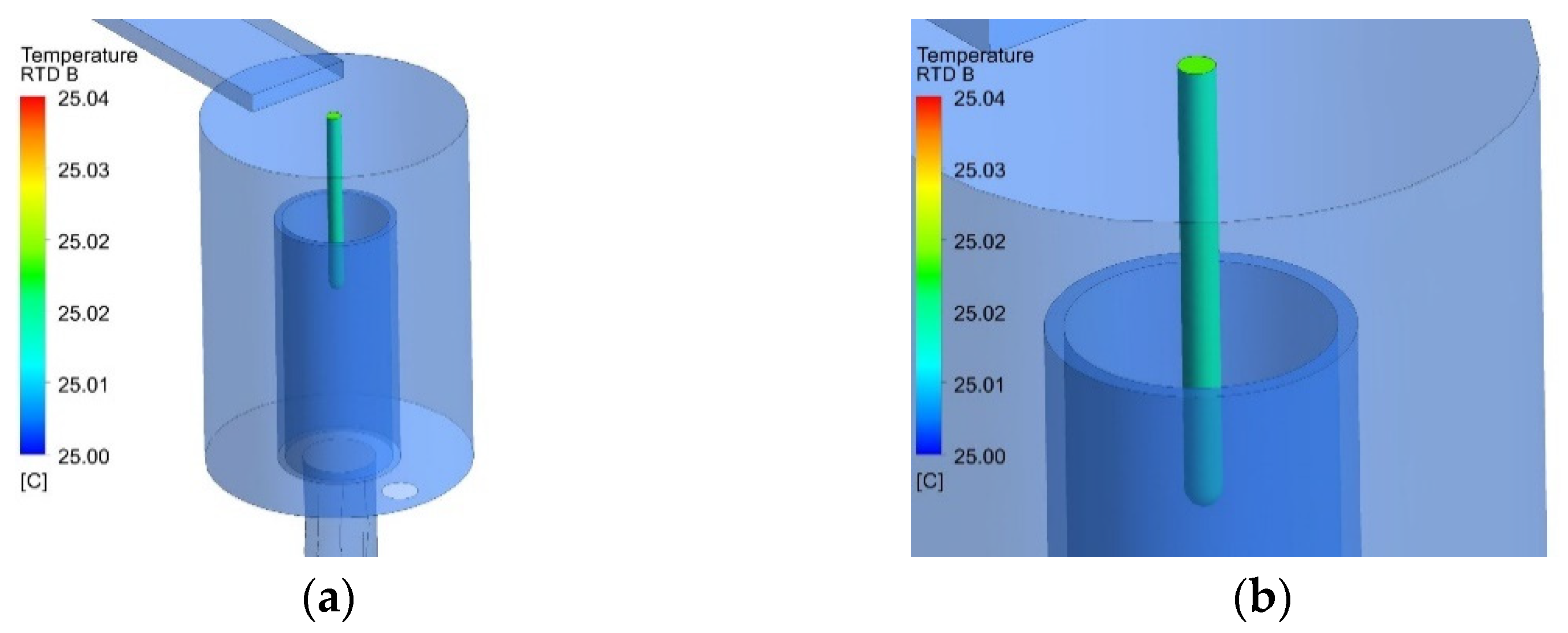
The processing of variables of interest in the software shows the temperature measured by the RTD sensor fitted inside the manifold (Figure 11) at the outlet of the draft tube. The dimensions of the simulated sensor are 4 mm in diameter and 50 mm long.
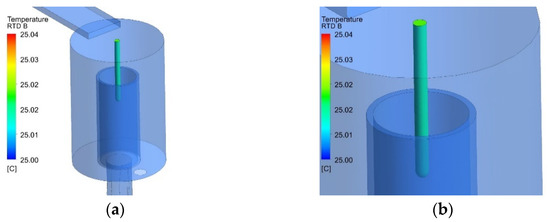
Figure 11.
Temperature, low-pressure section: (a) Isometric view (b) RTD Sensor, zoom.
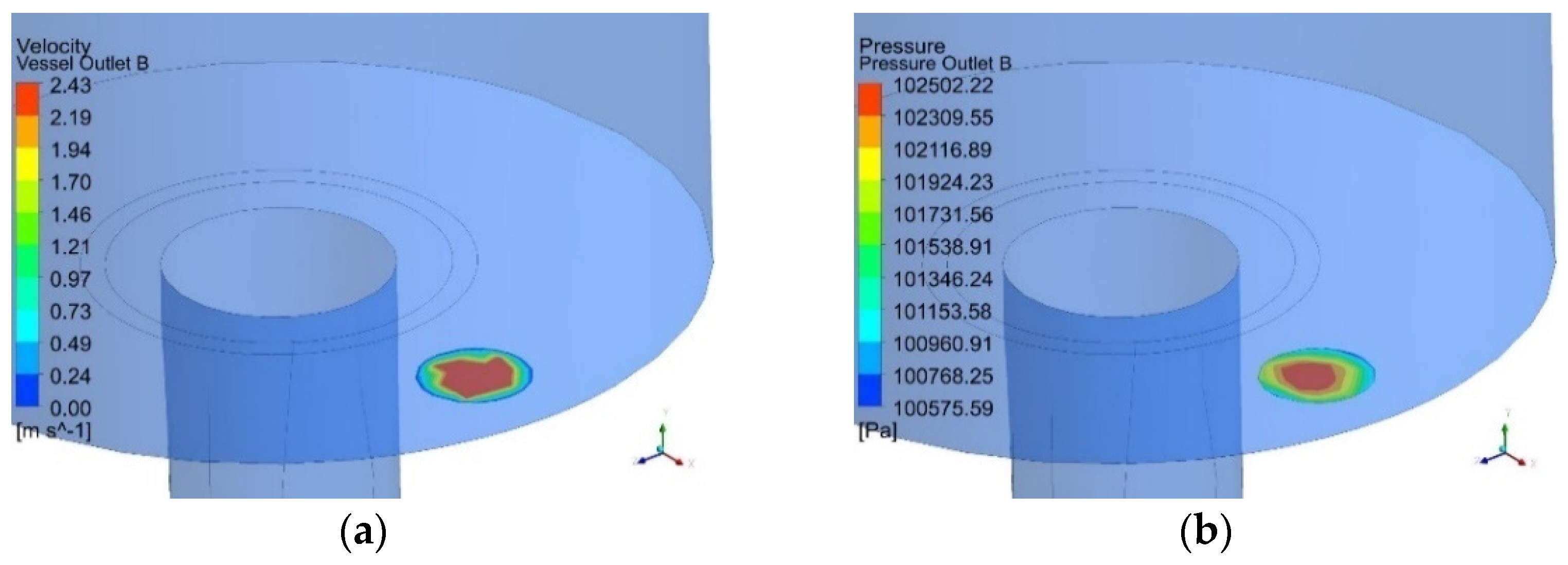
Figure 12 shows the velocity and pressure at the outlet of the manifold.
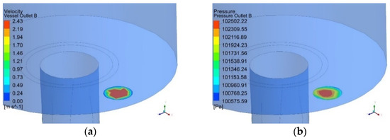
Figure 12.
Outlet location, (a) Velocity outlet, (b) Pressure Outlet.
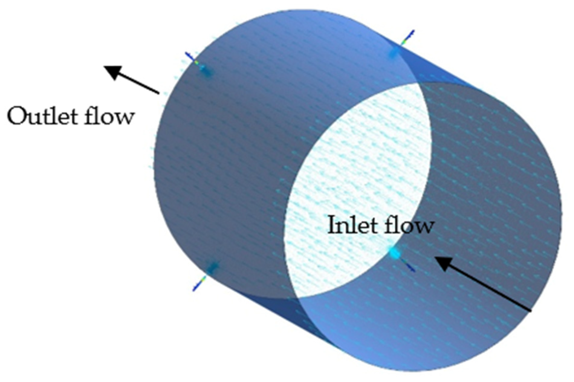
A view of the flow inlet through velocity vectors to the mixing chamber is shown in Figure 13. The total length of the collecting tubes is 4.06 m, equivalent to the outlet height of the draft tube for correct sampling in the zone, the diameter of the tubes is 30.8 mm or 1 ½ in., 10 inlet holes to the collection tube with a diameter of 10 mm satisfy the minimum dimensions required by the standard [2].
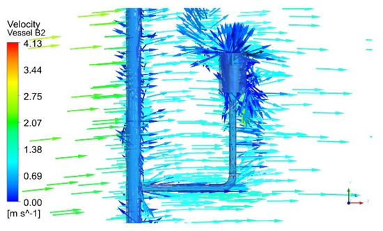
Figure 13.
Internal flow (velocity vectors), low-pressure section.
2.3. Application of Grid Convergence Index (GCI)
According to [22], the computer code used for CFD applications must be fully referenced, and previous code verification studies must be briefly described or cited. Appropriate methods could be selected to validate that CFD results do not depend on the quality or size of the grid. For the present study, the Grid Convergence Index (GCI) method was used.
The recommended procedure to calculate the fine-grid convergence index (GCI) is based on Equation (4)
where ea21 is approximated relative error, calculated by Equation (5). ϕ are the values of critical variables. For the present case, ϕ is the temperature (T11 or T21) at specific points in specific domains.
GCI21 = (1.25ea21)/(r21p − 1)
ea21 = |(Φ1 − Φ2)/Φ1|
r21p is the grid refinement factor r = hcoarse/hfine. It is desirable that this is greater than 1.3. The 21 subscripts correspond to the relationship between grid 1 (fine) and grid 2 (coarse); see Equation (6)
where “p” is the apparent order of the method used. For estimation of discretization error, it is necessary to define a representative cell, mesh or grid size “h” (mm). For example, Equation (7) is employed for three-dimensional calculations.
∆Vi is the volume and N is the total number of cells used for the computations. Another method to obtain the size of the grid (h) is analyzing the grid in the software used. This analysis can be conducted according to volume, the maximum/minimum length or the maximum/minimum side or the density of the grid.
r21p = h2/h1
In comparison with Equation (4), Roache [23] establishes that the grid convergence index (GCI) is based on Equation (8)
where ε is equivalent to ea21, and rp is equivalent to r21p. A summary and comparison of results for two grids are shown in Table 2 and Table 3.
GCIRo = 3|ε|/(rp − 1)
Table 2.
Summary of results, high-pressure section.
Table 3.
Summary of results, low-pressure section.
The grid convergence index (GCI) is adequate when the result is less than 1%, according to Roache. Despite the CGI differences between the authors, a value of less than 1% was obtained for both cases. Due to the presented results, it is possible to carry out the current study with the first generated grid.
2.4. Thermodynamic Method Application
The calculation of Hydraulic Efficiency (ηh) is defined by the ratio of the mechanical power (Pm) and the hydraulic power (Ph) of the turbine, respectively, as in Equation (9).
ηh = Pm/Ph
The mechanical power (Pm) of the turbine is calculated by the specific mechanical energy (Em), density (ρ) and the volumetric flow (QT) that passes through the turbine, as in Equation (10).
Pm = Em ∗ (QT ∗ ρ)
The hydraulic power (Ph), in contrast with the Pm, is obtained by means of the Specific Hydraulic Energy (Eh), as in Equation (11). The correction factor (ΔPh) is neglected since Urquiza [8] considered this factor in the presented results.
Ph = Eh ∗ (QT ∗ ρ) ± ∆Ph
The Em was calculated with the variables measured in the manifolds, such as pressure (p), temperature (T) and velocity (v), (see Equation (12)). The reference heights (z) are assigned for each manifold and the isothermal factor (ȧ), as well as the specific heat (Cp), are obtained from the annexes of IEC 60041, Appendix E physical data, Table EV and EVI [2] (Table 4), and an interpolation of the temperature and average pressure for each of the case studies.
Table 4.
Properties of water [2].
Finally, gravity (g) was obtained from Reference [8]. The subscripts 11 and 21 correspond to the manifolds in the inlet and outlet section, respectively. Similarly, T1 and T2 belong to the corresponding sections.
Em = [ȧ ∗ (p11 − p21)] + [Cp ∗ (T1 − T2)] + [(v112 − v212))/2] + [g ∗ (z11 − z21)]
The Eh is obtained by the properties measured in the main water flow (subscripts 1 and 2), Equation (13). Pressure (p), velocity (v) and height (z) are geodetic sampling points or reference points with respect to the height of the sea level at which the turbine is located. ρ, as well as ȧ and Cp, are obtained by interpolation.
Eh = [((p1 − p2))/ρ] + [((v12 − v22))/2] + [g ∗ (z1 − z2)]
The sampling points are observed in Figure 14, which is a general diagram of the turbine in question (original C.H. Temascal plane), as well as the areas in which the fluid properties are measured.
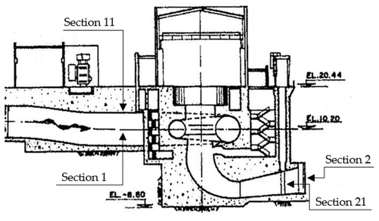
Figure 14.
Longitudinal view, measurement points [24].
According to [6], the mechanical energy (Em) is calculated by Equation (14). In this equation, ȧ is an isothermal factor of the water, p11, the inlet pressure in the diffuser, p21, the outlet pressure of the suction tube, T11, the inlet temperature of the suction tube, T20, the outlet temperature of the suction tube aspiration, z11, is a reference point for temperature measurement, and z1m is the reference point for measuring p11.
Em = [ȧ ∗ (p11 − p12)]
Em = [Cp ∗ (T11 − T20)] + [(v12 − v22))/2] + [g ∗ (z1m − z11)]
However, the variables for the present study were adapted to the previously established conditions, defining Em as Equation (15).
Em = [Cp ∗ (T1 − T2)] + [(v112 − v212))/2] + [g ∗ (z11 − z21)]
3. Results
3.1. Results of Thermodynamic Method
3.1.1. High-Pressure Section
For each of the different conditions and working sections, the temperature, velocity and pressure in the manifolds were obtained as required by IEC 60041. Similarly, the amount of volumetric flow that exits the manifolds located on the penstock and draft pipe was tested. As it is a stationary type of simulation, the value of temperature, pressure and velocity is obtained by exporting a series of values provided by the software in each of the locations of interest at the end of the numerical calculation (high- and low-pressure section). This series of values is averaged and shown below.
Table 5 contains the average temperature values in the four manifolds; Table 6 contains the average velocity and pressure values of the manifolds. Section 14.3.1 “General”; of the IEC-60041 standard establishes that the thermodynamic method for the average yield is based on the laws of thermodynamics, using the thermodynamic temperature ϑ in Kelvin (K). In case of temperature differences, the temperature can be directly expressed in Celsius (°C) degrees, as ϑ1 − ϑ2 = θ1 − θ2 [2].
Table 5.
Manifold´s temperature, high-pressure section.
Table 6.
Manifold’s velocity and pressure, high-pressure section.
3.1.2. Low-Pressure Section
The analysis of results in the low-pressure section (runner and draft tube) involves a comparison of the mechanical power and torque generated by the turbine for each flow condition (Table 7) in the software.
Table 7.
Comparison between mechanical power and torque, reported vs. simulated.
By demonstrating the same mechanical power and torque conditions, the results in the draft tube can be analyzed. The manifolds attached to the draft tube acquired samples of the main flow (water) to obtain the energy distribution at different points. Variables such as temperature, velocity and pressure, obtained in each of the containers, are shown in Table 8 and Table 9.
Table 8.
Manifold´s temperature, low-pressure section.
Table 9.
Manifold´s velocity and pressure, low-pressure section.
4. Discussion
The results obtained in the low-pressure section (draft tube) show that the direction of runner rotation (clockwise) and the geometry of the draft tube discharges water from a turbine, in addition to acting as an energy-recovery device, helping to improve the overall performance of the unit. It can also allow the downstream water level to be lower or higher than the equatorial plane of the turbine, depending on the needs of the facility. The draft tube, due to its divergent shape, causes a deceleration in the velocity of the water leaving the turbine, converting the kinetic energy of the fluid into pressure energy (Figure 15) [18].
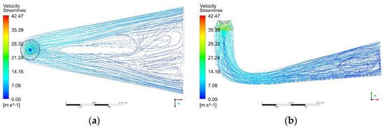
Figure 15.
Velocity streamlines on the complete turbine, (a) upper view, (b) lateral View.
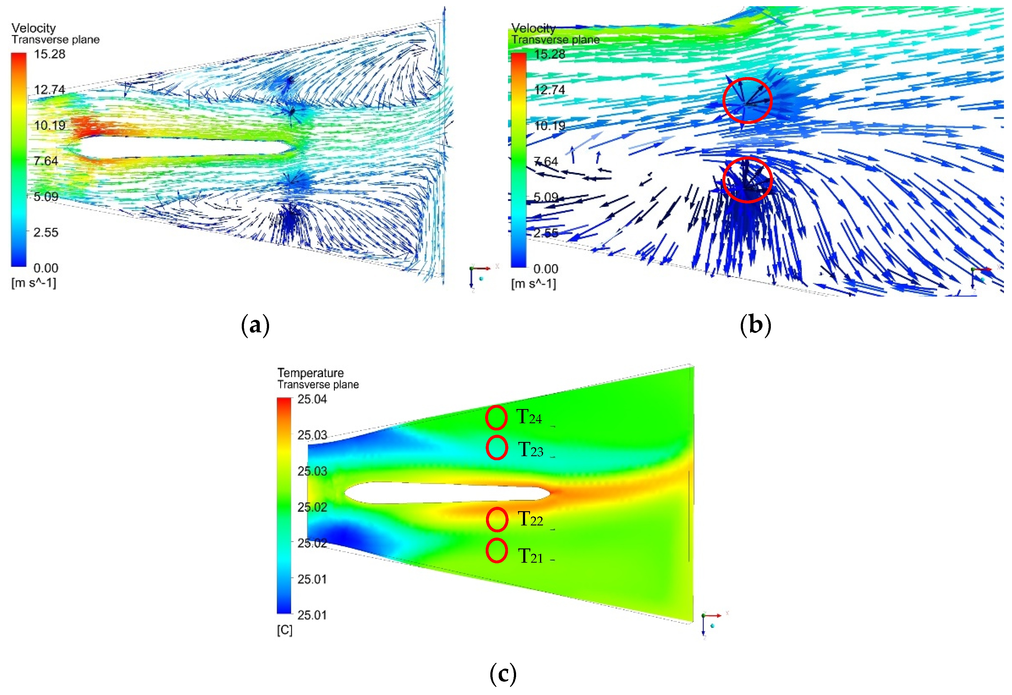
By coupling the manifolds in the draft tube, the flow distribution is affected, causing recirculation or vorticity in the area in which manifolds are located. The location of the manifolds is suggested by IEC-60041. Depending on the dimensions of probes, vorticity can be created behind the probes and then dissipated. The flow disturbance will be downstream once velocity, pressure, and temperature variables have been measured, so they cannot influence efficiency calculations. Therefore, the average temperatures in the manifolds T22 and T23 are slightly higher than the average temperature of T21 and T24, as derived from the flow distribution behavior in the turbine (Figure 16).

Figure 16.
Manifold´s in the draft tube, (a) Recirculation flow (normalized symbols), (b) Recirculation flow in manifolds, left section “zoom” (normalized symbols) (c) Temperature contour.
The summary of results obtained from the temperature differences T1–T2 (ΔT), Em, Eh, Pm, Ph and ηh, for different cases is presented in Table 10. Figure 17 and Figure 18 show the main comparison of the results, between what was reported in [18,24] and the current case study.
Table 10.
Summary of results, application of Thermodynamic Method.
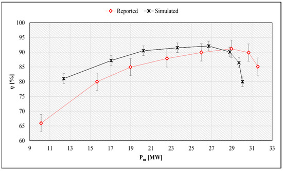
Figure 17.
Comparison, Reported hydraulic efficiency (Gibson method) vs. Simulated hydraulic efficiency.
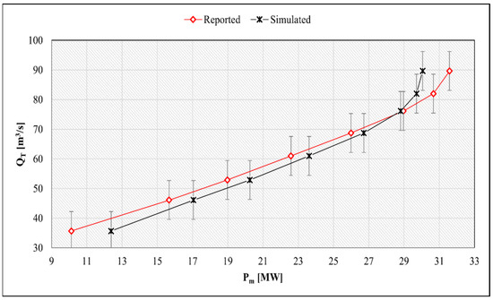
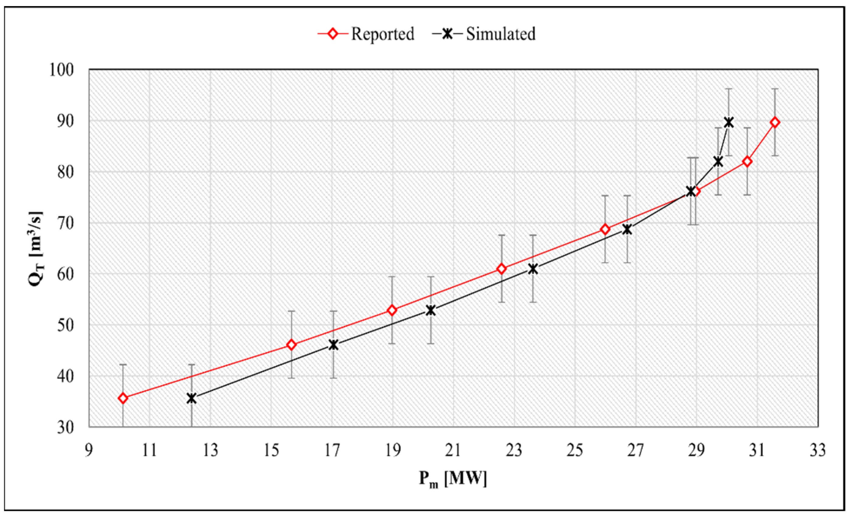
Figure 18.
Comparison of mechanical power generated, reported (Gibson method) vs. simulated.
CFD simulations are a proven tool to investigate hydraulic turbine performance, while measurements of some parameters, such as flow or pressure, are common in calculations of their efficiency. In the present study, the design of manifolds and CFD applications contribute to the assay, with sampling system (manifolds) and experimental measurement times in the power plant, complying with the criteria established to apply the TM to low-load turbines.
Experimental studies report that the water temperature at the turbomachine outlet must be higher than that at the inlet. With a lower temperature difference between the measurement sections, the maximum hydraulic efficiency is presented. According to those mentioned above [3], the difference between the efficiency curves is around 0.5%; however, for the present study, the maximum and minimum differences in efficiency are 15.12% and 1.09%, respectively, for the Gibson method (reported). As one of the most important variables for the study is the temperature on surfaces of principal components, such as the runner, penstock, draft tube, etc., and these are unknown, the domain was specified as adiabatic. As a result, there is a low-temperature increase in the water between the high- and low-pressure sections. These cause a low-energy exchange and higher efficiency than expected. If the temperature in these components was known, the boundary conditions could be set differently, and a lower efficiency would be expected in different cases. Likewise, the efficiency would present results closer to those reported. The hydraulic efficiency of the turbine is susceptible to temperature changes between one section and another. This sensitivity is presented with values up to 0.0001 K; the assumed temperature, or a change in temperature in any of the components, has a direct effect on efficiency.
The simulated TM presented differences in the mechanical power and efficiency; however, the behavior of the generated curve shows the same tendency as the curve in the experimental data obtained using the Gibson method (reported), presenting a gradual increase in efficiency until a maximum point is reached. This subsequently decreases. The results obtained for each operating condition are similar to those reported by the Gibson method, meaning an adequate comparison for the study of the proposed manifolds design, considering the head limits (less than 100 m), the amount of maximum volumetric input flow (89.67 m3/s), the type of turbine (Francis slow) and the specific speed of the turbomachine (less than 110). In future studies, the authors recommend developing transitory simulations for other operating conditions, as well as using the experimental test to measure temperature in the main components, and set different variables in the numerical simulations.
According to [3,12], the present study used a hybrid vertical detraction system and a mixing chamber for each tube, reducing the number of sensors that are required to facilitate installation in the low-pressure section. In addition, the manifolds proposed in the low-pressure section are compatible at different outlet heights for the draft tube, as it is only necessary to adjust the tube length.
5. Conclusions
Based on the location of the manifolds in the input and output sections, the proposed design of manifolds to measure properties of the main flow of a Francis-type low-head hydraulic turbine meet with the requirements suggested by the IEC—60041 Standard to carry out the Thermodynamic Method (TM) employing Computational Fluid Dynamics (CFD).
The distance from the turbine center to the measuring section is essential. The minimum distance set in the standard [2] is five times its maximum diameter, and the measurements show that it should be the absolute minimum. According to Figure 3, a shorter distance could improve energy distribution.
Using a mixing chamber inside the draft tube allows for a direct measurement of temperature in the principal flow at the outlet. In addition, inside the mixing chamber, there is a water flow concentrator, which helps to direct the flow into the temperature sensor, obtaining a direct measurement. The IEC-60041 establishes that the minimum number of tubes consists of two units that collect partial flows. However, increasing the number of tubes and manifolds at the outlet makes it possible to improve the temperature measurements. In this case, four manifolds were used in the low-pressure section. In both the left and right section, two manifolds were installed after the division to avoid a high recirculation or vorticity in the area in which manifolds are located.
On the other hand, the results obtained from the mechanical power and torque in the turbine runner were identical to those reported by the Gibson method (GM); however, the efficiency between the above methods is similar. To obtain results that are closer to reality, the numerical simulations used in CFD must be supplied from as many boundary conditions as possible (actual conditions). It is necessary to set the temperature on the surface of principal components so that the main flow of water makes contact via its passage through the turbomachine to the efficiency results, with the application of TM.
The efficiency calculation is higher under particular volumetric flow conditions (35.68 m3/s and 68.73 m3/s) compared to the efficiency reported when applying the GM. The maximum efficiency generated by the turbine applying the TM was 92.10%, corresponding to a flow of 68.73 m3/s. After the maximum efficiency point, the TM’s efficiency is lower than the GM’s.
Author Contributions
Conceptualization: L.L.C.G.; Investigation: E.O.C.M. and L.L.C.G.; Methodology: L.L.C.G.; Project administration: G.U.B.; Resources: G.U.B.; Software: L.L.C.G.; Supervision: G.U.B.; Writing—original draft preparation: E.O.C.M.; Writing—review & editing: L.L.C.G. and J.C.G.C. All authors have read and agreed to the published version of the manuscript.
Funding
This work is partly supported by the National Council for Science and Technology [Conacyt], CVU Number: 707755.
Acknowledgments
To Arturo Nava Torres, for his unconditional collaboration in the presented project. To the “Centro de Investigación en Ingeniería y Ciencias Aplicadas (CIICAp)”, for all facilities provided during my stay.
Conflicts of Interest
The authors declare no conflict of interest.
Glossary
| ȧ | Isothermal factor of water (m3/kg) |
| Cp | Specific heat capacity of water (J/kg °C) |
| Eh | Specific hydraulic energy (J/kg) |
| Em | Specific mechanical energy (J/kg) |
| g | gravity acceleration (m/s²) |
| p1 | Turbine pressure inlet (Pa) |
| p11 | Average pressure vessels, high-pressure section (Pa) |
| p2 | Turbine pressure outlet (Pa) |
| p21 | Average pressure vessels, low-pressure section (Pa) |
| Pe | Active generator power (MW) |
| Pf | Difference in losses in the bearings (%) |
| PgB | Loss in guide bearing (%) |
| Ph | Hydraulic power (MW) |
| Pm | Mechanical power (MW) |
| PtB | Loss in load bearing (%) |
| Q0 | Leakage flow (m3/s) |
| QT | Volumetric flow in turbine (m3/s) |
| T1 | Average temperature vessels, high-pressure section (°C) |
| T11 | Temperature, upper-right vessel (°C) |
| T12 | Temperature, upper-left vessel (°C) |
| T13 | Temperature, lower-right vessel (°C) |
| T14 | Temperature, lower-right vessel (°C) |
| T2 | Average temperature vessels, low-pressure section (°C) |
| T21 | Temperature vessel A (°C) |
| T22 | Temperature vessel B (°C) |
| T23 | Temperature vessel C (°C) |
| T24 | Temperature vessel D (°C) |
| v1 | Turbine velocity inlet (m/s) |
| v11 | Average velocity vessels, high-pressure section (m/s) |
| v2 | Turbine velocity outlet (m/s) |
| v21 | Average velocity vessels, low-pressure section (m/s) |
| z1 | Reference point high-pressure section (m) |
| z11 | Reference point in manifolds, high-pressure section (m) |
| z2 | Reference point low-pressure section (m) |
| z21 | Reference point in manifolds, low-pressure section (m) |
| ΔPh | Hydraulic power correction (W) |
| θ | Temperature (°C) |
| ΦP | Penstock diameter |
| δC | Uncertainty regarding the determination of the C-value (C = L/A) (%) |
| δQl | Relative uncertainty of measurement under final conditions by assessing flow intensification (leakage intensification) (%) |
| δQ | Total deviation of measurements of the flow in a systematic manner (%) |
| δrp | Error regarding the pressure change log (%) |
| δt | Error relating to measurement over time (%) |
| δΔA | Uncertainty regarding the change in pipe section due to the change in pressure (%) |
| δΔp | Uncertainty regarding errors in measuring pressure differences between sections of the pressure pipe (%) |
| δΔpf | Uncertainty regarding the decrease in pressure in the section of the pipe that generates hydraulic losses (%) |
| δΔρ | Uncertainty regarding the change in water density due to subsequent pressure change (%) |
| δρ | Uncertainty regarding the value of water density (%) |
| ηg | Generator efficiency (%) |
| ηh | Hydraulic efficiency (%) |
| ρ | Density (kg/m3) |
References
- Hulaas, H.; Vinnogg, L. Field acceptance tests to determine the hydraulic performance of hydraulic turbines, storage pumps and pump-turbines. Clause 14 Thermodynamic method for measuring efficiency, comments. In Proceedings of the International Group for Hydraulic Efficiency Measurements 2010, Roorkee, India, 21–23 October 2010. [Google Scholar]
- International Electrotechnical Commission 60041 (IEC 60041). Thermodynamic method for measuring efficiency. In Field Acceptance Tests to Determine the Hydraulic Performance of Hydraulic Turbines, Storage Pumps and Pump-Turbines, 3rd ed.; International Electrotechnical Commission: Geneva, Switzerland, 1991; pp. 293–319. [Google Scholar]
- Hulaas, H.; Nilsen, E.; Vinnogg, L. Thermodynamic efficiency measurements of Pelton turbines. Experience from investigation of energy/Temperature distribution in the discharge canal measuring section. In Proceedings of the 7th International Conference on Hydraulic Efficiency Measurements, Milan, Italy, 3–6 September 2008; p. 11. [Google Scholar]
- Patil, S.; Verma, H.; Kumar, A. Efficiency measurement of hydro machine by Thermodynamic method. In Proceedings of the 8th International Conference on Hydraulic Efficiency Measurements, Roorkee, India, 21–23 October 2010. [Google Scholar]
- Shang, D. Application research on testing efficiency of main drainage pump in coal mine using thermodynamic theories. Int. J. Rotating Mach. 2017, 2017, 5936506. [Google Scholar] [CrossRef] [Green Version]
- Kahraman, G.; Lütfi, Y.H.; Hakan, F.Ö. Evaluation of energy efficiency using thermodynamics analysis in a hydropower plant: A case study. Renew. Energy 2009, 34, 1458–1465. [Google Scholar] [CrossRef]
- Feng, X.; Hequet, T.; Muciaccia, F. Efficiency testing in Tai An (Shandong China) PSPP reversible units by means of thermodynamic method. In Proceedings of the International Group for Hydraulic Efficiency Measurements 2008, Milano, Italy, 3–6 September 2008. [Google Scholar]
- Karlicek, R.F. Analysis of uncertainties in the Thermodynamic Method of testing hydraulic turbines. In Proceedings of the IGHEM Seminar, Reno, NV, USA, 28–31 July 1998. [Google Scholar]
- Côté, E.; Proulx, G. Experiments with the thermodynamic method. In Proceedings of the International Group for Hydraulic Efficiency Measurements 2012, Trondheim, Norway, 28 June 2012. [Google Scholar]
- Gere, J.M.; Goodno, B.J. Mechanics of Materials; Cengage: Boston, MA, USA, 2009. [Google Scholar]
- Beer, F.; Russell, E.; DeWolf, J.; Mazurek, D. Mechanics of Materials; McGraw-Hill Education: New York, NY, USA, 2010. [Google Scholar]
- Mangla, M.; Khodre, N. Measurement of turbine efficiency by thermodynamic Method for field acceptance test of hydro turbine and Comparison with model test result. In Proceedings of the International Group for Hydraulic Efficiency Measurements 2010, Roorkee, India, 21–23 October 2010. [Google Scholar]
- Lugaresi, A.; Massa, A. Designing Francis turbines: Trends in the last decade. Water Power Dam Constr. 1987, 39, 23–32. [Google Scholar]
- Islam, R.J.; Siam, I.R.; Hasan, R.; Hasan, S.; Islam, F. A Comprehensive Study of Micro-Hydropower Plant and Its Potential in Bangladesh. Int. Sch. Res. Netw. 2012, 2012, 635396. [Google Scholar]
- Hatata, A.Y.; El-Saadawi, M.M.; Saad, S. A feasibility study of small hydro power for selected locations in Egypt. Energy Strategy Rev. 2019, 24, 300–313. [Google Scholar] [CrossRef]
- Prawin, A.M.; Jawahar, C.P. Design of 15 kW Micro Hydro Power Plant for Rural Electrification at Valara. In Proceedings of the 1st International Conference on Power Engineering, Computing and CONtrol, PECCON-2017, Tamil Nadu, India, 2–4 March 2017. [Google Scholar]
- Ole, G.D.; Torbjørn, K.N.; Brandåstrø, B.; Håkon, H.F.; Wiborg, E.J.; Hulaas, H. Comparison between pressure-time and thermodynamic efficiency measurements on a low head turbine. In Proceedings of the 6th International Conference on Innovation in Hydraulic Efficiency Measurements, Portland, OR, USA, 30 July–1 August 2006. [Google Scholar]
- Castro, L.; Urquiza, G.; Adamkowski, A.; Reggio, M. Experimental and numerical simulations predictions comparison of power and efficiency in hydraulic turbine. Model. Simul. Eng. 2011, 2011, 146054. [Google Scholar] [CrossRef] [Green Version]
- Castañeda, M.E.O.; Castro, G.L.L.; Urquiza, B.G.; Alcántara, M.J. Diseño de un recipiente colector para medición de eficiencia teórica en turbinas hidráulicas. In Proceedings of the SOMIM Conference, Sinaloa, Mexico, 18–20 September 2019. [Google Scholar]
- Urquiza, B.G.; Kubiak, S.; Adamkowski, A.; Janicki, W. Condiciones Previas para la Medición de Flujo y Cálculo de Eficiencia de la Unidad No. 4 en la C. H. Temascal, Tech. Rep. 76P/DM/CIICAp. 2005. [Google Scholar]
- Lecture 7: Turbulence Modeling Introduction to ANSYS Fluent, Sales Conference Theme and Team Building. Available online: https://www.academia.edu/36090206/Lecture_7_Turbulence_Modeling_Introduction_to_ANSYS_Fluent (accessed on 5 December 2021).
- Celik, B.I.; Ghia, U.; Roache, P.J.; Freitas, C.J.; Coleman, H.; Raad, P.E. Procedure for estimation and reporting of uncertainty due to discretization in CFD applications. J. Fluids Eng. Trans. ASME 2008, 1, 130. [Google Scholar]
- Roache, P.J. Perspective: A method for uniform reporting of grid refinement studies. J. Fluids Eng. 1994, 116, 405–413. [Google Scholar] [CrossRef]
- Urquiza, B.G.; Kubiak, S.; Adamkowski, A.; Janicki, W. Resultados de Medición de Flujo y Cálculo de Eficiencia de la Unidad No. 4 en la C. H. Temascal, Tech. Rep. 77P/DM/CIICAp. 2005. [Google Scholar]


Publisher’s Note: MDPI stays neutral with regard to jurisdictional claims in published maps and institutional affiliations. |
© 2021 by the authors. Licensee MDPI, Basel, Switzerland. This article is an open access article distributed under the terms and conditions of the Creative Commons Attribution (CC BY) license (https://creativecommons.org/licenses/by/4.0/).