Comparison of Flexibility Factors and Introduction of A Flexibility Classification Using Advanced Heat Pump Control

Abstract

With the increasing use of renewable energy, the energy flexibility of buildings becomes increasingly important regarding grid support. Therefore, there is a need to describe this flexibility in a concise manner. For the characterization of building energy flexibility, flexibility factors can be used. The comparison of a selection of existing flexibility factors shows that they are not easy to use or understand for designers and users. A simplification is necessary. The aim of this study is to introduce a flexibility classification that is easy to understand and shows in an easy way if a building already uses the lowest energy cost level or if further improvement is possible. The classification expresses the annual energy costs in colored classes: green (class A) for lowest up to red (class D) for highest level. Basically, the flexibility classes can be derived for any metric of interest, in this paper examples are shown for energy costs and CO_2eq emissions. The results given are based on the simulation of load management scenarios with different penalty signals applied for the heat pump operation of a residential building.

1. Introduction

1.1. Background

The worldwide increasing temperatures have an impact on natural and human systems. It is assumed, that the global warming is likely to reach 1.5 °C above pre-industrial levels between 2030 and 2052 if the current rate continues [1]. The European Green Deal is the European Union’s concept against climate change [2]. The three targets are (a) climate-neutrality by 2050 (b) engagement of citizens and all parts of society (c) reduction of greenhouse gas emissions by at least 55% below 1990 levels by 2030. The Green Deal requires a transformation of the energy supply from fossil fuels to renewable energy. This increases the use of wind and solar energy. Their fluctuating power generation requires changes in the electric power system [3]. Moreover, as the penetration of heat pumps [4] and photovoltaic systems [5] increases, buildings increasingly challenge the electric power system.

To balance variable energy supply and consumption, flexibility is needed. Flexibility can be provided by equipment and operation of buildings. Residential smart appliances (washing machines, tumble dryers, dishwashers, domestic hot water buffers and electric vehicles) can be used for flexibility [6], but only a very limited amount can be shifted through the control of domestic electrical appliances [7,8]. Both thermal and electrical storage can be used for flexibility. The use of thermal energy storage like water tanks [9] and thermal building mass [10] are common. In [11] it is stated that the size of the storage tank and the temperature difference between the in- and outlet of the storage tank have a large impact on flexibility. Less common are phase change or thermochemical material tanks [12] and the effects of internal thermal mass like furniture [13]. The building envelope insulation level has the largest impact on shifting heating energy followed by thermal mass [14]. Buildings with a low heat demand can shift smaller amounts of energy with a delay of several hours while buildings with a high heat demand have a higher shiftable heating load but only for a short time [15]. Electrical energy storage increases self-consumption of photovoltaic yield [16]. Electric load shifting with pre-cooling of residential buildings can also reduce peak load demand [17]. The study focusses on low thermal mass residential buildings, such as timber-frame houses typical for the US. With different pre-cooling strategies at least 50% of the on-peak cooling loads can be shifted away from the peak period window 4–8 pm. A comparison of four storage options (batteries, fuel switch, water tanks and thermal building mass) for an office building is given in [18]. Batteries are reported to be the most effective and efficient option both in the heat pump and CHP system. The load shifting potential of batteries is related to the capacity. Fuel switch for peak demand improves grid support but increases gas consumption, also. The flexibility based on water tanks depends on the ratio of thermal storage capacity and thermal power of the heating system. With a CHP smaller water tanks can be used compared to a heat pump system. Large amounts of thermal energy can be stored by thermal mass with a high-inertia heat emission system (concrete core conditioning). Due to the low temperature differences this is preferable for heat pump systems.

There are different methodologies to quantify the energy flexibility of buildings. They have in common that the energy consumption can be delayed or anticipated, usually based on a “penalty signal”. The flexibility can be qualified by the shifted amount of time and power [19]. In general, the basis for flexibility is a building with a heat pump and a photovoltaic system. Load management makes it possible to use the different storage options for operating the building in a grid supportive way. The penalty signals can be set by the grid suppliers, e.g., price, CO_2eq emissions or primary energy. Advanced control systems will operate the building based on the chosen penalty signal. The load will be shifted, e.g., to times with low energy prices or CO_2eq emissions. Different examples (33 cases) of the use of flexibility in buildings are given in [20]. To obtain energy flexibility, a wide range of control strategies are used. Flexibility can be obtained e.g., with a simple on/off control of a heat pump during a daily predefined period. A more complex control is a rule-based control that contains some restrictions such as switching the heat pump when the electricity price is below a certain limit or forcing the hot water tank to overheat when there is a photovoltaic surplus. Including weather forecasts or occupancy behavior a model-based control is needed. In [20] the examples are 57% rule-based, 37% model-based and 6% use other sources for flexibility. Different control strategies and algorithms are explained for 12 cases in [21]. A very broad overview of characterization and quantification methods and applications of flexible buildings is given by [22].The buildings flexibility potential can be found by simulation, experimental or real life set up’s and can be expressed in flexibility factors [23]. In general, three types of energy flexibility can be observed: (a) the temporal flexibility, (b) the amount of energy or power that can be shifted and (c) the associated cost of activating the flexibility [24]. In [25], flexibility factors are introduced which express the flexibility in regard to load-shift ability, power adjustment potential, energy efficiency and cost efficiency for single buildings. Most of the factors compare two cases: without/with load management. Flexibility factors can also be used for building clusters [26]. A data driven model that simulates a generic building cluster is introduced in [27]. When the number of buildings increases, the uncertainty of the energy flexibility decreases.

1.2. Motivation

As mentioned above, several studies were done in regard to energy flexibility, but in general each study uses one approach only [10,18,28]. A compilation of 20 different flexibility factors for single buildings is given in [25] and in [26] 16 flexibility factors are listed for building clusters. Previous studies found focus only on one flexibility factor each or list flexibility factor values without further information about validation ranges and examples. The study reported on here, however, evaluates a selection of flexibility factors based on the same building and HVAC system. This allows a comparison of the usage of different flexibility factors regarding clearly defined validation ranges and metrics used. Based on the comparison, the validity of the results and ease-of-use for designers is assessed. Such a comparison and assessment are missing to date.

A key aspect is to determine a factor or derive a classification which is easy to understand and use in the design and operating phase. An easy-to-use factor/classification increases the knowledge and awareness of building flexibility performance and can foster the ongoing energy supply transformation.

1.3. Specific Objectives

The energy flexibility of a small multi-family dwelling in regard to the demand response aimed at optimizing towards different penalty signals is evaluated. Following penalty signals are considered: electricity costs (high/low tariff, spot market prices), CO_2eq emissions and self-consumption. The optimization is realized by controlling the heat pump accordingly. The penalty signals’ impact on different ratings is shown. The flexibility is expressed in different flexibility factors. These factors are compared, and their applicability is evaluated. Based on the findings, a new flexibility classification including a corresponding Flexibility Classification Factor (FCF) is developed and introduced. Together, they express the energy flexibility and related energy cost, CO_2eq emissions or other metrics of the building to the designer and/or building user in a more readily usable way. The study does not focus on increasing the energy efficiency but focuses on using flexibility.

The paper is structured as follows: In Section 2 the methodology is introduced along with the investigated building, flexibility factors, penalty signals and control strategies. Then, in Section 3 the results for the flexibility factors are presented. Next, in Section 4 the results for the flexibility factors are analyzed and the new flexibility classification and a corresponding factor is introduced. Finally, the last section concludes the findings of this study and outlines plans for future work.

2. Methodology

2.1. Multi-Family Dwelling

The studied multi-family dwelling comprises three apartments with a heated area of 320 m². The building has a high thermal insulation level (Swiss label Minergie-P) and a high thermal mass based on a concrete and aerated concrete construction. The thermal building simulation model is validated with monitored data [8,29,30,31]. After validation, the internal loads are changed according to Swiss Standard values [32]. The mechanical ventilation has a heat recovery value of 80%. This leads to an annual space heating of 15.4 kWh/m². Basic values of the building are shown in

Table 1. Properties of the residential building [35].

Property	Value
U-value, ext. walls	0.12 W/(m2 K)
U-value roof	0.09 W/(m2 K)
U-value floor	0.10 W/(m2 K)
U-value windows	0.75 W/(m2 K)
g-value, windows	50%
Glazed part of wall (area rated)	23%
Solar control (blinds)	Not applicable
Shading (surrounding buildings)	yes
Thermal capacity (with Rsi), [36]	63 Wh/(m2NetFloorArea K)
Const. air exchange rate (mech. ventilation)	0.39 h−1
Climate, [37]	DRY Buchs-Aarau (CH)

. The inverter-controlled ground-source heat pump (min./max. 5–18.5 kW) has a nominal power of 8.8 kW with a coefficient of performance of 4.9 (B0/W35, part-load operation at 50 Hz). The reference characteristic is derived from a CTA Optiheat model [33]. The ground-source heat pump model used is based on the air-source heat pump described in [34]. The heat pump provides the heat required for heating and domestic hot water.

The domestic hot water tank (800 L) is heated daily in two different block times (1 h and 2 h duration). The daytime of the two block times depends on the penalty signal. The source temperatures of the heat pump and freshwater are based on monthly mean values given in Figure 1. Each Saturday, the domestic hot water tank is heated up for 2 h to 65 °C for Legionella protection. During the remaining time the tank is heated to a maximum of 53 °C. The daily overall tank heating duration of 3 h is sufficient. The tank temperature stays mainly between 45–50 °C. Only during a few hours the temperature drops down to 40 °C, which still ensures a sufficient tap temperature. The stochastic water draw profile method of ESP-r is used [38]. The total daily draw amount is set to 175 L of hot water.

The real building is equipped with a roof mounted photovoltaic system of 20 kWp and a slope of 10° facing south.

2.2. Penalty Signals

2.2.1. Selection

In this study, the penalty signals “electricity price” and “CO_2eq emission” are used. The objective for the price-based penalty signal is to shift the heat pump operation in times with low electricity prices to minimize the electricity costs. Two scenarios are considered: (1) high/low tariff (daily block values) and (2) spot market prices. CO_2eq emission efficiency is the goal of the CO_2eq driven penalty signal. The load management shifts the electricity demand for the heat pump operation to times when CO_2eq emission levels in the grid are low. The additional aim for a building with a photovoltaic system is to achieve a high level of self-consumption. In this case the penalty signal for the heat pump operation is an allowed time span during the day.

2.2.2. High/Low Tariff

Today, energy suppliers in Switzerland typically offer high and low tariffs for electricity consumption. The tariffs differ slightly between suppliers. In this paper, the tariffs of [39] are used (

Table 2. Low and high tariff for 2020 incl. tax. [39].

Rariff	Electric Energy [Rp/kWh]	Levies [Rp/kWh]	Total [Rp/kWh]
Hight tariff Monday–Friday 6 a.m.–8 p.m.	8.80	27.99	36.79
Low tariff all other times	7.15	15.35	22.50
Flat tariff (24/7)	7.95	26.30	34.25
feed in tariff for PV yield	-	-	14.00

). To minimize energy costs with such a high/low tariff the main consumption must occur during the night.

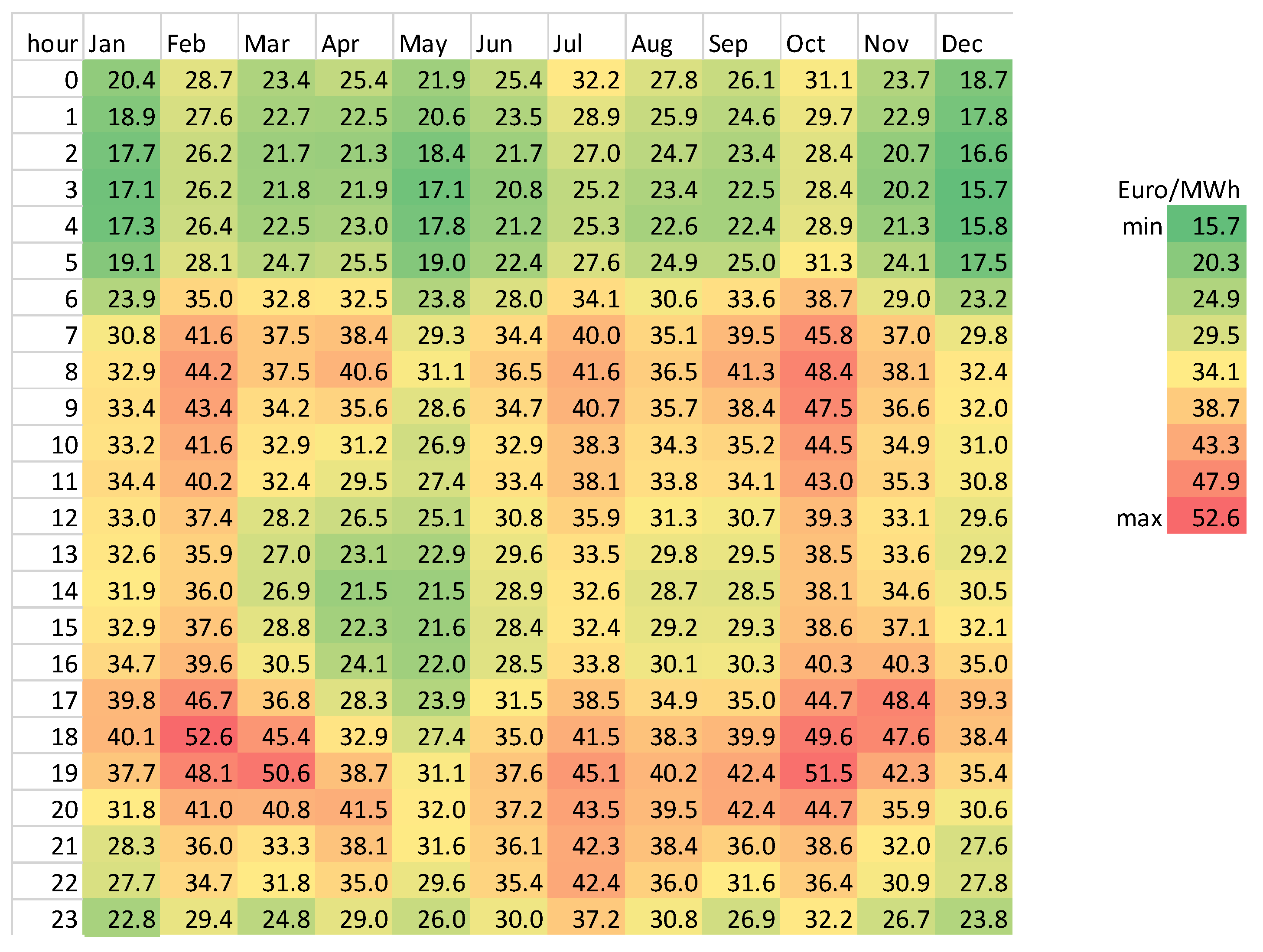
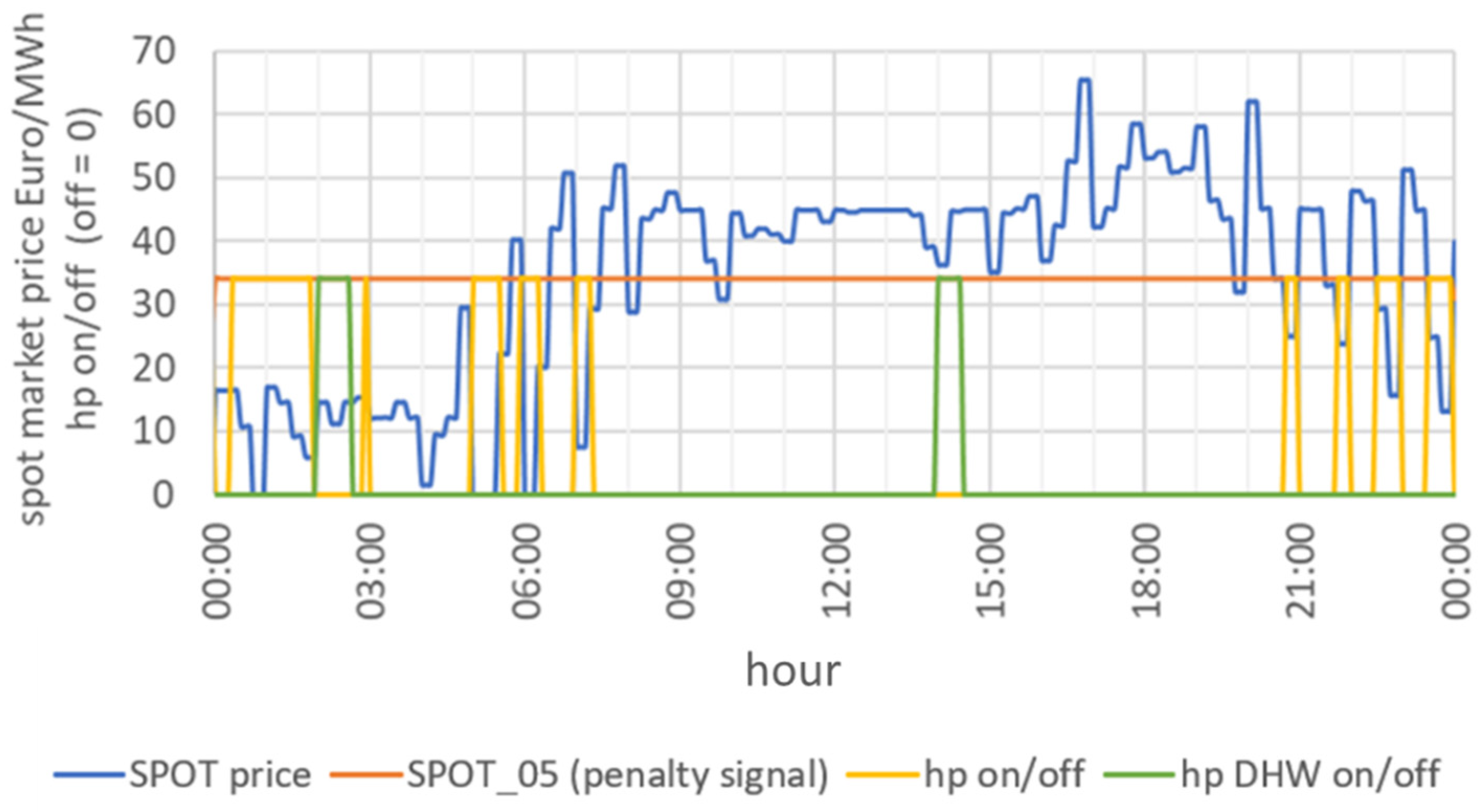
2.2.3. Spot Market Prices

As no Swiss spot market prices are available at the time of the study, 15-min spot market prices from Germany for the year 2015 are used [40]. Figure 2 shows the monthly mean spot market prices for each hour of the day. There is no clear seasonal trend for low/high prices. The spot market prices are mainly low during the night (green color) and high during the day (red color). With the penalty signal of spot market prices, the goal is to use the energy in low price periods. In general, it is favorable to operate the heat pump at night and early in the morning. Also, a short window during early afternoon shows low spot market prices. As the spot market prices are pure energy prices and all levies are missing, the energy prices are supplemented with the levies for the flat tariff of (Table 2) for the sake of comparison.

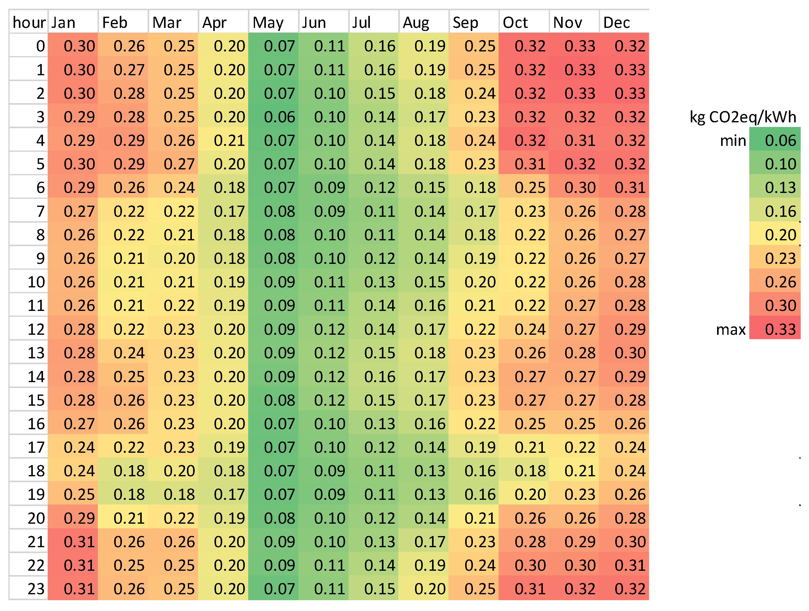
2.2.4. CO_2eq Emissions

Renewable energy but also nuclear power plants cause low CO_2eq emissions. Since nuclear power plants are inflexible and are used for base load coverage, one can assume a continuous base load of CO_2eq emissions from these plants. The CO_2eq emissions on top depend on the amount of renewable energy in the grid. Therefore, the CO_2eq emissions can be used as an indicator of the renewable energy amount in the electricity mix of the grid. Low CO_2eq emissions are considered to correlate with a high amount of renewable energy. CO_2eq emissions are related to the CO_2eq coefficients. Low CO_2eq coefficients lead to low CO_2eq emissions and vice versa. Figure 3 shows the monthly mean values for each hour of the day for the CO_2eq coefficients of the Swiss electricity mix in 2015/2016 [41]. The green color indicates low and the red color high CO_2eq coefficients. The lowest CO_2eq coefficients can be seen for the whole month Mai. In general, the CO_2eq coefficients are lower during the summer months May through August than in winter from September to April. The CO_2eq coefficients fluctuate during each day. Both low and high coefficients can appear during nighttime and daytime. However, low coefficients are increasingly found during daytime. The mean monthly daily course shows the lowest CO_2eq coefficients during 6 am–8 pm. Attempting to draw from the grid during times with low CO_2eq coefficients favors energy consumption during daytime.

2.2.5. Self-Consumption

In the case of self-consumption optimization, the heat pump is operated in such a way that as much of the solar yield of the local photovoltaic system is used as possible. The heat pump operates during the day only. This reduces the grid feed-in of the excess yield and lowers grid draw during the high energy price period.

2.3. Flexibility Factors

2.3.1. Introduction

The buildings’ flexibility can be expressed by various flexibility factors. In this study, seven flexibility factors are considered. Some of the flexibility factors need a base case and a penalty-controlled case. All factors illustrate the ability to shift the energy from high to low prices or CO_2eq emissions. Almost all factors use rated electricity energy. The rating parameters are high/low tariff, spot market price or CO_2eq emission. For transparency reasons, in this paper the flexibility factors are described for energy costs only but remain the same for CO_2eq emissions. The factors are all computed for each day of the year and afterwards aggregated to a yearly value.

Table 3. Summary off all used flexibility factors.

Flexibility Characteristics	Valid Range	Grid Supportiv, if…	Which Values are Needed?
GSC	>0	<1	Values of electricity/penalty (time step), daily sum of electricity, daily mean value of penalty
RIB	0–1	Low value	Values of electricity (time step), lowest/highest daily penalty signal
FF	−1–1	High value	Values of electricity (time step), first/forth quartile of daily penalty
FI	≤1	High pos. value, neg. value = worsening	Values of electricity/penalty (time step), base and penalty-controlled case
Sflex	0–1	High value	Values of electricity (time step), base and penalty-controlled case
SCR	0–1	High value	Values of electricity and PV yield (time step), daily sum of PV yield
AR	0–1	High value	Values of electricity and PV yield (time step), daily sum of electricity

summarizes the main parameters of the flexibility factors.

2.3.2. Grid Support Coefficient (GSC)

The Grid Support coefficient (GSC) [18] compares the electricity consumption rated with the real-time energy price compared with the daily sum of electricity consumption rated with the daily mean energy prices as given in Equation (1). GSC is accepted for values equal to or greater than zero. If the electricity consumption is always in low price periods, e.g., lower than the daily mean price, GSC is smaller than 1. GSC = 1 means that the daily electricity consumption is done within the daily mean price. If GSC is greater than 1 the daily consumption takes place at high electricity prices. In [18] two GSC types are presented: GSC_abs and GSC_rel. The GSC used in this paper corresponds to GSC_abs.

$$GSC=\frac{{\sum }_{i=1}^n(E_{el}^i·p^i)}{\left({\sum }_{i=1}^n{E}_{el}^i\right)·\overline{p}}(-)$$

(1)

where $E_{el}^i$ is the electricity consumption in time step i, (kWh), and pⁱ the price in time step i, (Rp/kWh). $\overline{p}=\frac{1}{n}\sum _{i=1}^n p^i$ is the mean value of the price, (Rp/kWh, 100 Rp = 1 CHF Swiss currency) and n the total number of time steps.

2.3.3. Relative Import Bill

The Relative Import Bill (RIB) [28] compares the achieved reduction of the electricity bill/costs to the maximum reduction possible as given by Equation (2). The maximum reduction is computed with the lowest and highest electricity price of the day. RIB is accepted from [0;1]. The smaller the value, the more electricity is consumed at times of low electricity prices.

$$RIB=\frac{{\sum }_{i=1}^n(E_{el}^i·p^i)-{\sum }_{i=1}^n(E_{el}^i·p_{min})}{{\sum }_{i=1}^n(E_{el}^i·p_{max})-{\sum }_{i=1}^n(E_{el}^i·p_{min})}(-)$$

(2)

where p_min/p_max: highest and lowest electricity price of the day, (Rp/kWh).

2.3.4. Flexibility Factor (FF)

The Flexibility factor (FF) [10] uses the price classification in daily price quartiles given in Equation (3). The electricity price is divided in three categories: low, mid and high price. A low price corresponds to a price in the first quartile (price ≤ 25% of all prices during one day). A high price is defined to be higher than the third quartile (price > 75% of all prices during one day). In [10] the quartiles are evaluated over two weeks. In this paper the quartiles are computed daily to control the heat pump according the real pricing. The range of FF is from [−1;1]. If the heat pump operates equally in times with high and low prices FF = 0. FF = 1 when consumption occurs only during times with low prices. Electricity consumption with high prices leads to FF < 0.

$$FF=\frac{{\sum }_{i=1}^n{(E_{el}^i·p^i)}_{q1}-{\sum }_{i=1}^n{(E_{el}^i·p^i)}_{>q3}}{{\sum }_{i=1}^n{(E_{el}^i·p^i)}_{q1}+{\sum }_{i=1}^n{(E_{el}^i·p^i)}_{>q3}}(-)$$

(3)

where q1/q3 are the first and third quartile.

2.3.5. Flexibility Index (FI)

The Flexibility Index (FI) [42] compares a base case with a penalty controlled case (Equation (4)). FI is defined for values less than or equal to one. Values < 0 mean that the penalty-controlled case operated by higher energy cost than the base case. These cases are not preferable. The target is a high positive value whenever possible closed to one. The higher the value the more energy is shifted compared to the base case.

$$FI=1-\frac{{\sum }_{i=1}^n{(E_{el}^i·p^i)}_{flex}}{{\sum }_{i=1}^n{(E_{el}^i·p^i)}_{ref}}(-)$$

(4)

where flex/ref: case with/without penalty control.

2.3.6. Shifted Flexible Load (S_flex)

The Shifted Flexible Load (S_flex) shows the amount of shifted energy of a penalty controlled case compare to a base case [43]. S_flex is defined in the range [0;1] (Equation (5)). A value of 1 means that all electricity is shifted compared to the reference case, a value of 0 indicates that no electricity is shifted.

$$S_{flex}=\frac{{\sum }_{i=1}^{n}max{(E_{el,ref}^i-E_{el,flex}^i,0)}_{}}{{\sum }_{i=1}^n{E}_{el,ref}^i}(-)$$

(5)

2.3.7. Self-Consumption Rate (SCR) and Autarky Rate (AR)

The Self-Consumption Rate (SCR) shows the amount of directly used PV yield in the building (Equation (6)). The Autarky Rate (AR) describes the amount of electricity consumption that is directly covered by PV yield (Equation (7)). Both parameters have the range from [0;1] (Equations (6) and (7)). The higher the value the more PV yield can be used directly.

$$SCR={\displaystyle \sum }_{i=1}^n\frac{S{C}_{}^i}{P{V}_{yield}^i}(-)$$

(6)

$$AR={\displaystyle \sum }_{i=1}^n\frac{S{C}_{}^i}{E_{el}^i}(-)$$

(7)

where SCⁱ = min ($E_{el}^i$; $P{V}_{yield}^i$) is the self-consumption in time step i, (kWh) and $P{V}_{yield}^i$ is the PV yield in time step i, (kWh).

2.4. Control Strategies and Evaluation Criteria

The merit of the heat pump control is investigated for five different penalty signals (

Table 4. Investigated penalty signals for heat pump control [44].

Penalty Signal	Allowed Operation Times for Heat Pump (without Block Times for Domestic Hot Water)	Block Times for Domestic Hot Water
DEMAND	On demand (base case)	5–6 a.m., 1–3 p.m.
LT	Low tariff only, this excludes Monday to Friday 6 a.m.–8 p.m.	4–6 a.m., 8–9 p.m.
SPOT_05	When spot market price ≤ daily mean price	2–4 a.m, 2–3 p.m.
CO2_05	When CO2eq emission coefficient ≤ daily mean coefficient	8–9 a.m., 6–8 p.m.
DAY	Block time during daytime: 7 a.m.–6 p.m.	5–6 a.m., 1–3 p.m.

). Each result is computed with the three ratings: high/low tariff (HTLT), spot market price (SPOT) and CO_2eq emissions (CO_2eq) and analyzed for each flexibility factor. Only the electricity consumption for the heat pump is analyzed.

Regarding the photovoltaic system three scenarios are considered:

• no photovoltaic system
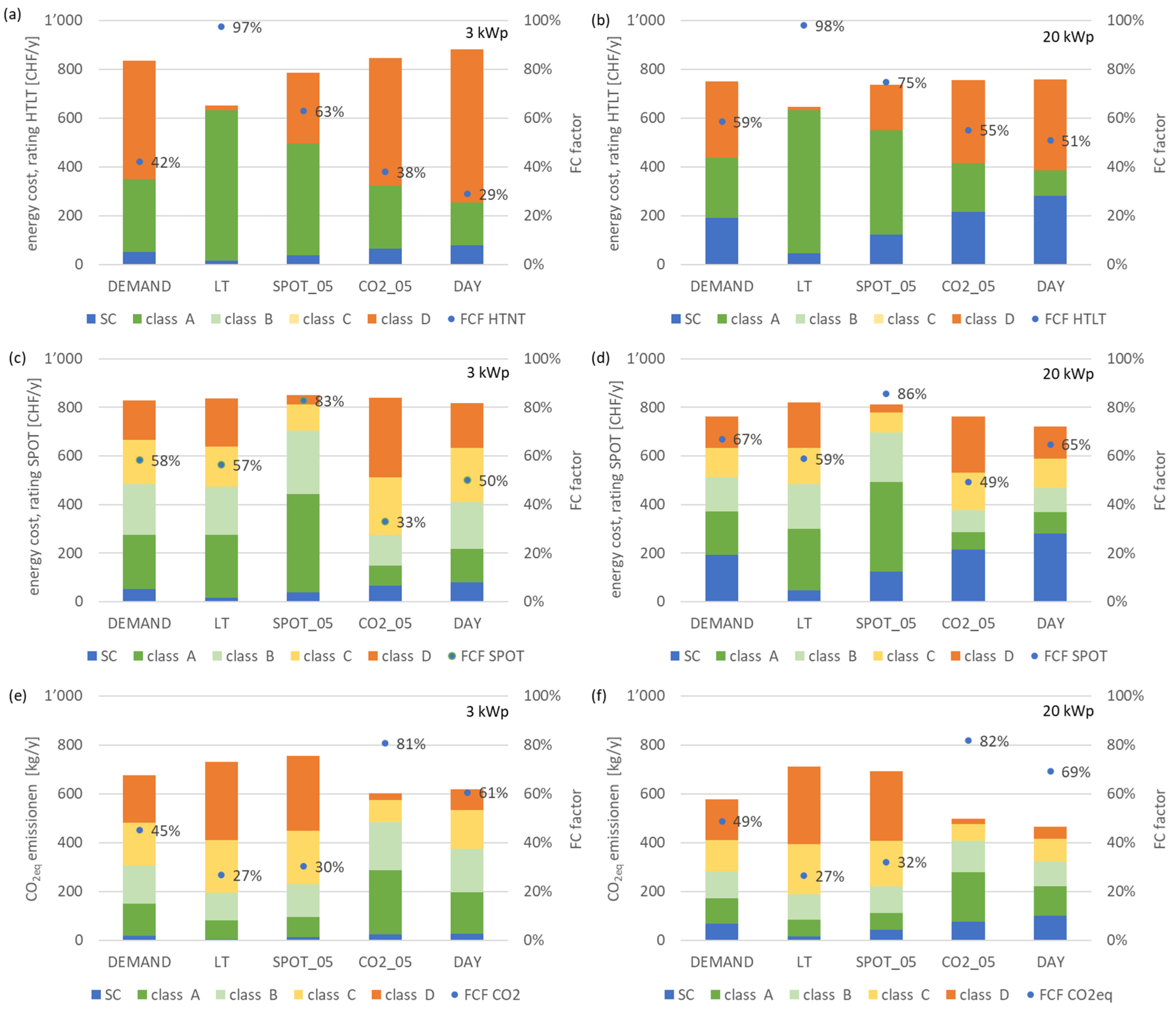
• small photovoltaic system: PV yield can cover the annual electricity demand of the heat pump (3 kWp: yield 2950 kWh/y, demand: 2700 kWh/y)
• large photovoltaic system: system of the real building (20 kWp: 18590 kWh/y)

It is assumed that the PV yield can be completely used for the heat pump when needed. It is also assumed that the heat pump has a base load/standby of 10 W when it is “off”.

2.5. Numerical Setup

The simulations are carried out using the dynamic thermal simulation program ESP-r [45]. The model consists of 15 thermal zones. Explicit models of the modulating heat pump and the domestic hot water storage are used. The heat pump run time control according to Table 4 was set up in the plant domain using pre-defined temporal data profiles for high-low tariff, spot-market prices and CO_2eq emissions coefficients. The flexibility factors are calculated in the post processing.

Figure 4 shows a control example of one simulated winter day with the penalty signal SPOT_05. The orange line represents the daily mean spot market price, and the heat pump is allowed to run for heating if the current spot market price (blue line) is below this line. The yellow line shows when the heat pump is on/off for heating. If needed, longer on-periods would have been possible during the early morning hours. Also, three short periods were not used during the day. The DHW generation is during the allowed times (green line). The same methodology also applies to the other penalty signals. The controls presume that the penalty signal values are known in advance. Additionally, it is verified that the operative temperatures of all zones are always above 20 °C.

The time resolution is 5 min for the building behavior and 1 min for the heat pump and thermal behavior of the domestic hot water storage. For the analysis a full year is considered. A pre-simulation period of 30 days is used to initialize the thermal conditions of the building model.

3. Results and Analysis

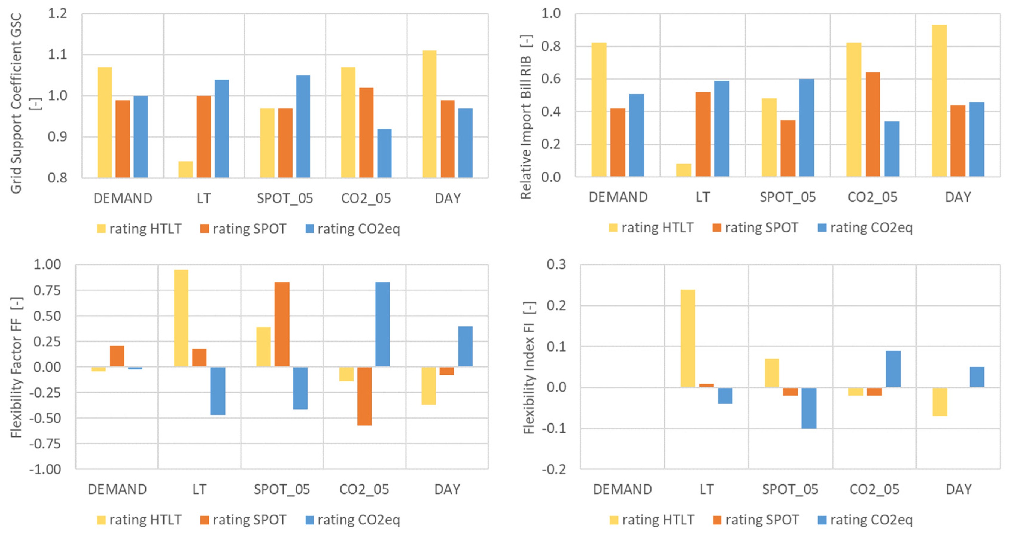
3.1. Without a Photovoltaic System

The performance of controls based on the proposed penalty signals analyzed for the flexibility factors is shown in Figure 5 and Figure 6. Figure 5 shows the absolute shifted energy costs/CO_2eq emissions and relative shifted amount of load for all penalty signals and ratings compare to the base control. The left figure shows that the penalty signal LT leads to a large saving when rated with HTLT. This behavior is expected because this penalty signal corresponds to the rating. When the control LT is rated with SPOT only a very small amount can be saved. LT means that the heat pump runs during the night only. Although the spot market prices are mainly low during the night too, the impact isn’t nearly as large as for HTLT. Therefore, only a small amount can be saved. The nocturnal operation also means that the heat pump operates in times with high CO_2eq emissions. The LT optimized heat pump control increases the CO_2eq emissions compared to the base case.

The SPOT_05 optimization shows marginal savings when rated with HTLT and a small additional expense when rated with SPOT. This leads to the conclusion that the heat pump demand is partly shifted into the night and partly shifted to different hours during the day compared to the base case. The SPOT_05 optimization significantly increases CO_2eq emissions.

The CO_2eq control favors heat pump operation during the day, which means during low CO_2eq emissions periods but more operation during high tariff and high spot market prices. Optimizing the penalty signal DAY means operating the heat pump during the day only. Without a photovoltaic system this means that the energy consumption during high tariff increases. The SPOT rating barely changes between the controls DEMAND and DAY.

The controls LT, Spot_05 and CO2_05 shift approximately 80% of the energy compared to DEMAND (Figure 5, right). In the case of DAY, only 40% can be shifted. That means that in the base case the heat pump operates already with a large share during the day.

The general behavior described for Figure 5 can also be found in Figure 6 for the other flexibility factors. GSC, RIB and FF show the flexibility potential used. If these values are close to the lower limit for cost or CO_2eq emissions, the flexibility potential is exhausted. Otherwise, there is some potential left:

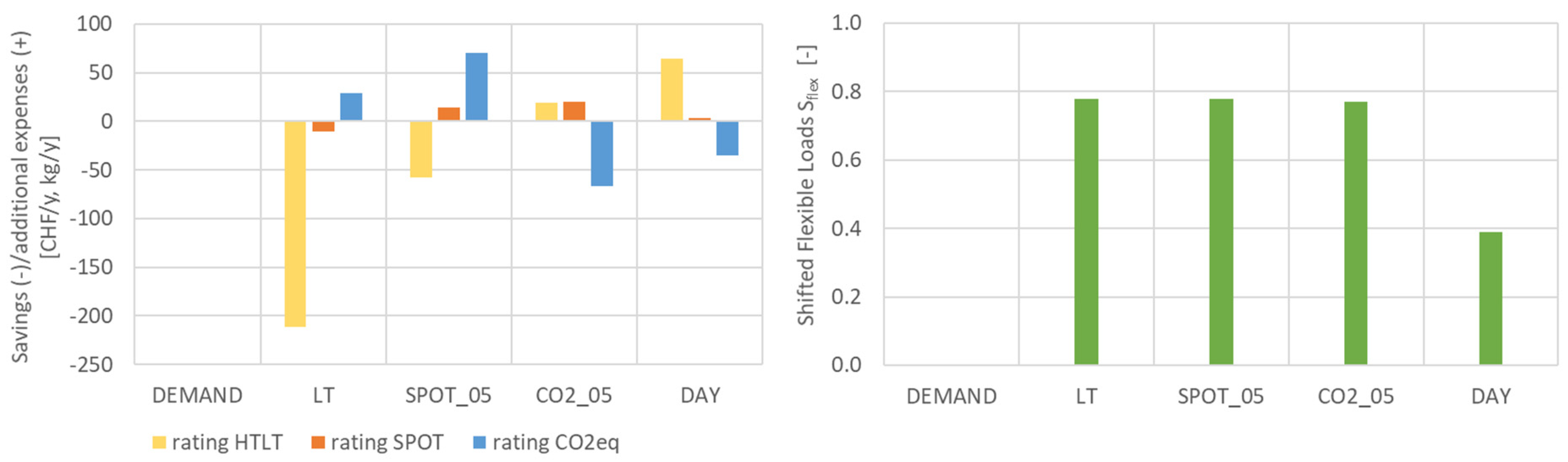
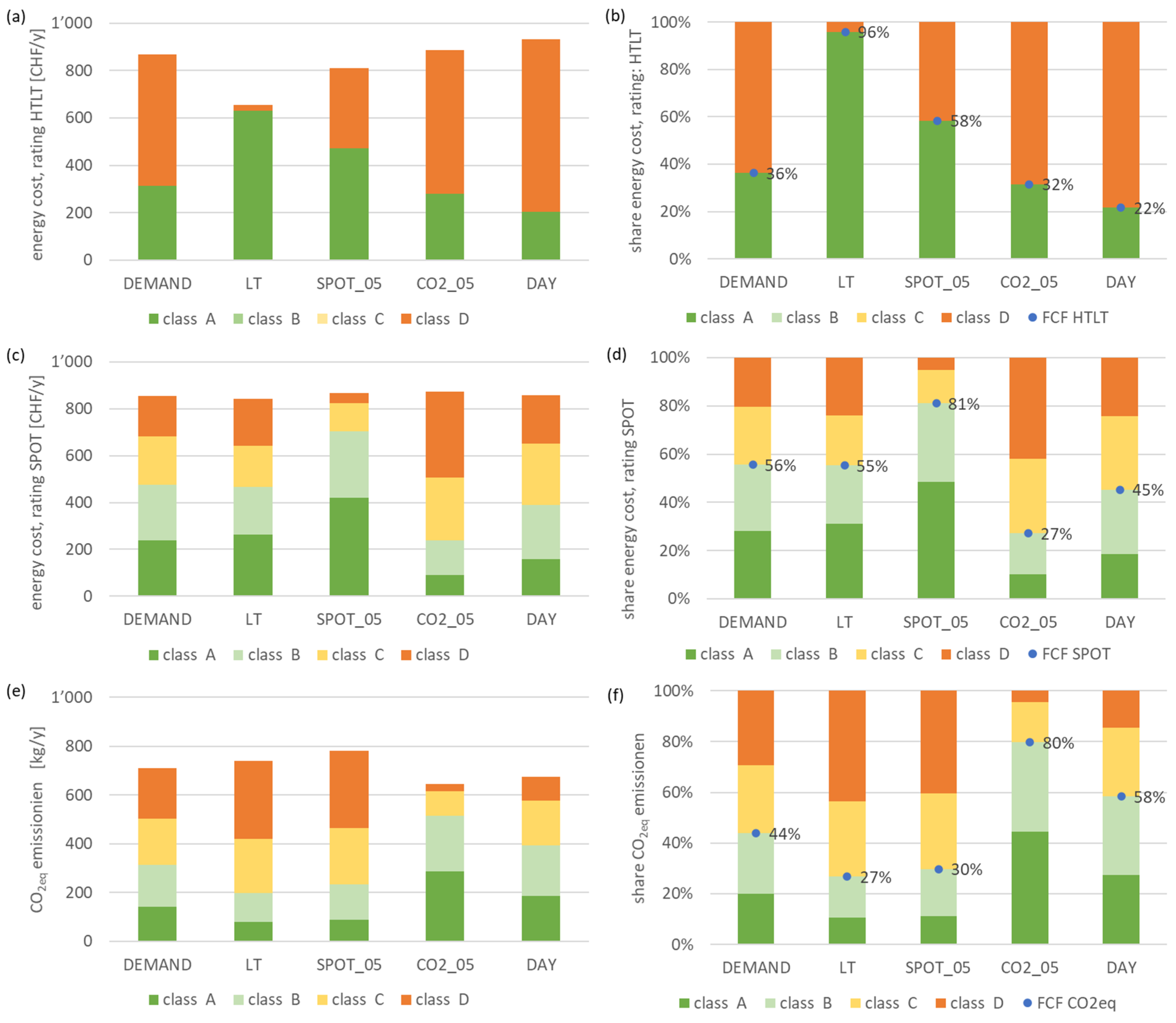
• DEMAND: GSC and RIB show that the energy consumption is more often in times with hight than in low tariff (yellow, GSC > 1, RIB > 0.5). High and low tariffs are counterbalanced in FF (FF ≈ 0). The SPOT and CO_2eq rating is nearly counterbalanced with a slight tendency towards low tariffs (orange/blue, GSC ≈ 1, RIB ≈ 0.5 and FF ≈ 0).
• LT and SPOT_05: rated with HTLT and SPOT the consumption shifts mainly to lower prices but this increases the CO_2eq emissions compared to DEMAND.
• CO2_05 and DAY: the consumption increases with rating HTLT and SPOT but decreases with rating CO_2eq.

FI includes the comparison of a penalty and base control. Controls and corresponding ratings show energy shifting to lower energy costs or CO_2eq emissions compared to the base case. One exception is the control SPOT_05 and the SPOT rating. It shows a slight increase in energy costs and CO_2eq emissions. The SPOT control and rating barely has an impact on FI. FI mirrors the course of savings and additional expenses in Figure 5 (left side) compared to a base case.

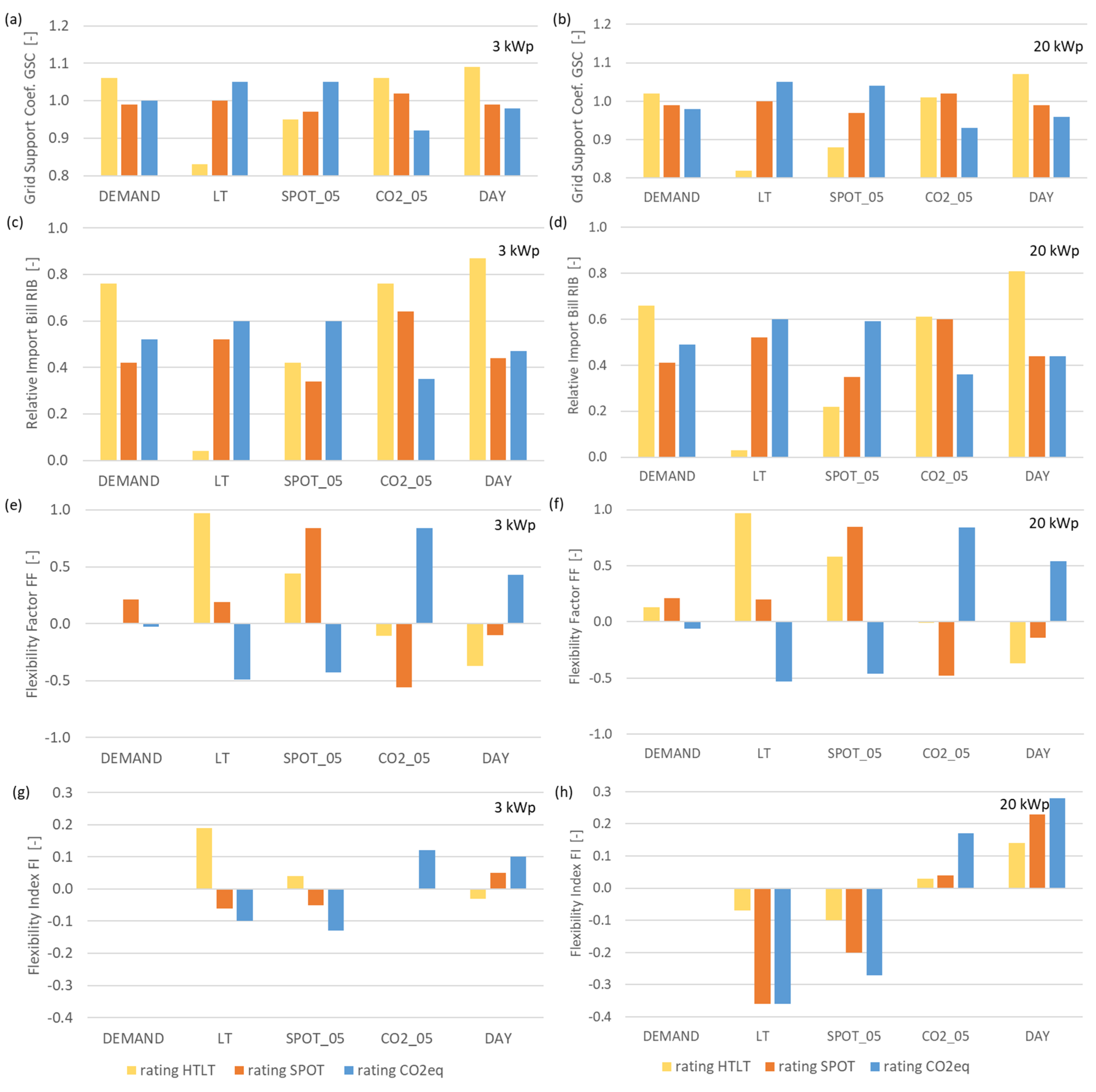
3.2. With a Photovoltaic System

Results for the flexibility factors GSC, RIB, FF and FI taking a 3 kWp (left column) and 20 kWp (right column) photovoltaic system into account are shown in Figure 7. The production cost for self-consumption is set to 20 Rp/kWh [46] and CO_2eq emissions are set to 0.072 kg/kWh [47].

The results with the 3 kWp PV system are very similar to the results without a PV system. Such a small PV system has a very low winter yield which results in a quite low self-consumption. The large PV system with 20 kWp results in a higher winter yield which has a large impact on GSC, RIB and FF rated with HTLT. Due to the higher self-consumption, which usually takes place at high tariff times, energy costs are reduced, which has a positive effect on the flexibility parameters. In general, the penalty signals LT and SPOT_05 shift a large part of energy consumption compared to the base case. The penalty signals CO2_05 and DAY only shift a small part of the energy consumption. The results are mirrored in self-consumption rate and autarky rate (Figure 8). SCR and AR increase with an increase in daytime operation of the heat pump:

• The 3 kWp system shows a low SCR and AR because of a low yield, particularly in winter.
• The high yield of a 20 kWp system results in a low SCR but clearly in a high AR.

In general, it is found that the price-focused controls shift the heat pump operation mainly into the night. The CO_2eq emissions and self-consumption focused controls shift the operation mainly into the day. The most extreme shifts are caused by high/low tariff and optimization of the self-consumption. Spot market prices and CO_2eq emissions vary during the day, however not to the extent of strictly grouped high and low values in the night or day. Nevertheless, the price controls lead to lower energy costs but higher CO_2eq emissions and low self-consumption and vice versa.

4. Discussion and Further Development

4.1. Flexibility Factors

Even though the methodology of the various flexibility factors is very different, the results are very similar. GSC, RIB and FF give information about the cost or CO_2eq allocation even if there is only one case available. This is an advantage compared to FI and S_flex that always need two cases to be derived. The advantage of RIB and FF compared to the other factors is that they have ranges of validity which are easy to understand. Minimum and maximum values are defined. The mean of the minimum and maximum values shows the counterbalance in costs or CO_2eq emissions. It can be viewed as slightly confusing that a high value of RIB means high energy costs while a high value of FF means low energy costs.

Above mentioned factors give different information. GSC, RIB, FF and S_flex show the flexibility for a given situation depending on the validity range. If this value is closed to the lower limit for cost or CO_2eq emissions (GSC, RIB, FF) or maximum shifted loads (S_flex) the flexibility potential is exhausted. FI however addresses the savings and additional expenses compared to a base case. It does not provide information about the flexibility potential.

SCR and AR are only possible when a PV system is available. High values of SCR and AR indicate that the heat pump operating times correspond with times of PV yield. In order to be able to interpret SCR and AR, the heat pump demand and PV size must be taken into account.

The flexibility factors considered so far are based on the fact that a certain value is exceeded or undercut or has to be increased or decreased. Because of the fixed range of validity, the factors RIB and FF are basically suitable to describe the flexibility of a building—but for experts only. For acceptance and widespread use in practice, a more comprehensible presentation is required. A parameter which provides information both on available flexibility and savings potentials compared to a base case at the same time would be preferable. In the following, such a parameter is introduced.

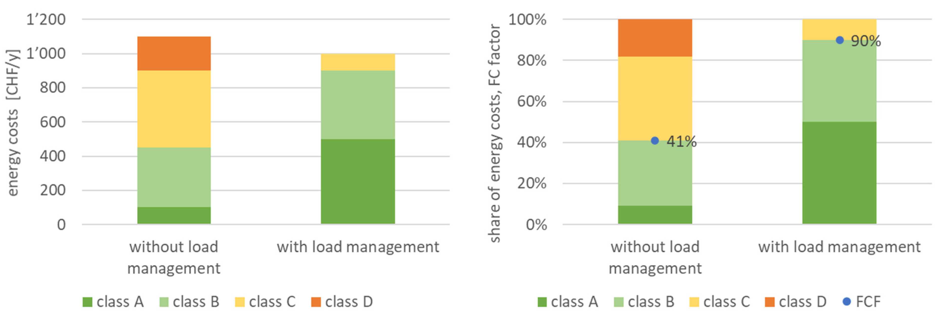
4.2. Flexibility Classification (FC)

4.2.1. Introduction

To describe flexibility in a way that is more useful for practitioners, a flexibility classification is proposed. This classification immediately shows the total annual energy costs and whether the energy is mainly purchased at high or low prices. If all energy is purchased at low prices, the shifting goal is reached. In general, the flexibility classification includes four classes, A–D, and is based on the daily price quartiles (

Table 5. Flexibility classification based on daily price quartiles.

Class	Energy Consumption When	Quartile
A	price lower ≤ 25% of all prices during one day	q1
B	price between 25% and ≤50% of all prices during one day	q2
C	price between 50% and ≤75% of all prices during one day	q3
D	price > 75% of all prices during one day	>q3

). The energy costs of each class are computed on a daily basis and are then aggregated to an annual value.

An example of the flexibility classification without and with load management is shown in Figure 9. The classification colors make it easy to understand. Green signals indicate low prices (class A/B) and yellow/red indicate high prices (class C/D). The reader can directly see the distribution of the energy costs. An all-green result signifies that all energy consumption is during hours with energy costs less than the daily median value. This clearly signals that the building in question is flexible. In the best possible case of an all-dark-green result (class A), the energy consumption is in times during the lowest 25% of the daily prices. This means the building is very flexible. The lower the red area fraction is, the lower the energy costs and the higher the flexibility of the building.

The classification can be used for one case only or for comparison of different cases. Therefore, savings and additional expenses compared to a bases case can be derived.

On the right side, Figure 9 also shows the Flexibility Classification Factor (FCF) as defined in Equation (8), below. The basis for FCF is the assumption that it is desirable to consume energy only during times with energy costs lower than the daily mean value. In other words, the flexibility classification must be in the green classes A and B. Thus, FCF is 100% (=1) when all energy costs are in classes A and B. This corresponds with a high use of flexibility and a depleted flexibility potential. FC is 0% (=0) when all energy costs are in classes C and D. In this case, unused flexibility potential is available. The higher the flexibility of a building, the higher the FCF value. The flexibility classification and the corresponding FC factor allow to address the flexibility potential and the savings and additional expenses compared to a bases case. Both parameters can also be used for CO_2eq emissions or other penalty signals.

$$FCF=\frac{{\sum }_{i=1}^n{(E_{el}^i·p^i)}_{q1}+{\sum }_{i=1}^n{(E_{el}^i·p^i)}_{q2}+{\sum }_{i=1}^n{(S{C}_{}^i·p_{SC}^i)}_{}}{{\sum }_{i=1}^n{(E_{el}^i·p^i)}_{}+{\sum }_{i=1}^n{(S{C}_{}^i·p_{SC}^i)}_{}}(-)$$

(8)

where $p_{SC}^i$: price for self-consumption in time step i (Rp/kWh), q1/q2 are the first/second quartile.

4.2.2. Application without Photovoltaic System

The flexibility classifications and FCF values are shown in Figure 10 for cases without a PV system. The rating HTLT only shows classes A and D because of the tariff profile (Figure 10, top). With the rating HTLT and penalty signal LT, the energy cost compared to the base case can be reduced by −24% (Figure 10, top). The FC factor increases to 96%, because almost the entire energy demand takes place during low tariff periods. The remaining 4% high price class D includes the standby during periods with the heat pump switched off. The flexibility potential is used up. Rating with SPOT and penalty signal SPOT_05 (Figure 10, middle) increases the annual costs by about 2% compared with the base case but at the same time increases the use of low prices (FCF = 81%). There is some flexibility potential still available. Looking at rating and penalty signal CO_2eq emissions, savings of about −9% compared to the base case can be achieved (Figure 10, bottom). FCF increases to 80%. The flexibility potential is not completely used up.

The different class colors show the cost compositions. The user can directly see if the heat pump often operates in high price times (orange color) or not. The goal is to operate the heat pump in low price times (green colors) as much as possible. Cost-controlled cases have higher FCF values when rated with costs than when rated with CO_2eq emission and vice versa. Or, generally spoken, if the rating corresponds with the penalty signal, high FCF values occur.

4.2.3. Application with Photovoltaic System

With a PV system, the flexibility classes A to D are extended with the “class” self-consumption. FCF includes self-consumption, anyway, as given in Equation (8). The values obtained with the small 3 kWp PV system are almost the same as without a PV system (Figure 10 and Figure 11, left). As already mentioned above, the reason for this is the low winter yield. Considering a 20 kWp PV system the self-consumption increases strongly. This can be seen in the increased share of self-consumption (SC, blue color) and the decrease of energy costs and CO_2eq emissions (Figure 11, right). The self-consumption increases FCF, also. One exception is the penalty control LT. When the heat pump mainly runs during the night, the PV yield cannot be used much.

4.3. Generalization of Flexibility Factors and Classification

All discussed flexibility factors are based on values which can be derive from any building. Each building has an electricity demand and at least electricity prices will be available. The factors can also be used for buildings without a heat pump. The increasing use of smart meters makes load profiles more and more available. This data can be combined with the electricity price, CO_2eq emissions or any other available metric. Smart home systems can easily show daily, weekly, monthly and annual flexibility factors. The advantage of the newly introduced flexibility classification and corresponding factor over the other flexibility factors is that it makes it very easy for the user to classify the building performance. The aim is to reach a classification factor as close to one as possible, readily identifiable by the user due to a high ratio of green coloured classes A and B in the evaluation. For any building which features a PV system, the self-consumption (blue coloured class) can be evaluated. The added value of the classification is that not only that the flexibility potential can be described, but also savings and additional expenses compared to a base case can be derived.

The flexibility factors and classification discussed in this study can not only be used for single buildings but also to describe or classify the flexibility of a cluster of buildings. They are not limited to residential buildings.

Basically, it is entirely possible to adapt the factors and classification to parameters other than electricity consumption, e.g., heat consumption or power. The flexibility factors and classification can be widely used.

5. Conclusions and Future Work

To quantify the flexibility potential a number of flexibility factors are analyzed and a new flexibility classification and corresponding factor is proposed. For the analysis, load management of a heat pump in a small multi-family dwelling is used. In general, it is found that the price-focused controls shift the heat pump operation mainly into the night. The CO_2eq emissions and the self-consumption focused controls shift the operation mainly into the day.

All flexibility factors considered give the same general flexibility results, despite different calculation methodologies. But the practicability of these factors varies due to different limit values. Only RIB and FF have defined minimum and maximum values which makes them easier to understand compared to the other factors. However, for acceptance and widespread use in practice, a more comprehensible presentation is required and a new flexibility classification and corresponding factor is proposed. The flexibility classification divides the energy costs or CO_2eq emissions into four classes, A to D, from low to high values. These well-defined flexibility classes together with the FCF and the possibility of a label-like illustration of the classes lead to an added value compared to the raw flexibility factors. Information about flexibility potential and annual costs or CO_2eq emissions are made available. This makes the flexibility of a building more tangible for designers and building users and thus leads to more understanding and acceptance.

The flexibility factors and classification discussed here can be used both for single buildings and for building clusters, as they are solely based on electricity demand and a rating value. Moreover, a heat pump is not necessary, but of course offers flexibility for load management in regard to a given penalty signal in an electricity-based evaluation.

Further investigation is needed concerning the impact of higher heat demands (lower insulation standards) on the newly introduced flexibility classification and factor. A high heat demand necessitates longer heat pump operation times which will be mirrored in higher electricity costs and lower flexibility. Other aspects such as electrical equipment and artificial lighting, cooling load or a combination with other energy carries could be addressed.

Also, the new flexibility classification should be introduced to and discussed with architects, designers and policy makers. If it is accepted, the flexibility classification can be used in the design and operation phase. For the future, it is conceivable that a requirement for flexibility will be imposed as part of a building label, e.g., either by requiring a specific class (e.g., A or B) or defining a level of FCF to be achieved e.g., FCF ≥ 0.75. Also, ratings for flexibility, e.g., one star: FCF ≥ 0.50, two stars: FCF ≥ 0.75, three stars: FCF ≥ 0.90 are conceivable.

References and Notes

1. Masson-Delmotte, V.; Zhai, P.; Pörtner, H.-O.; Roberts, D.; Skea, J.; Shukla, P.R.; Pirani, A.; Moufouma-Okia, W.; Péan, C.; Pidcock, R.; et al. “Summary for Policymakers”, in Global Warming of 1.5 °C; An IPCC Special Report on the Impacts of Global Warming of 1.5 °C above Pre-Industrial Levels and Related Global Greenhouse Gas Emission Pathways, in the Context of Strengthening the Global Response to the Threat of Climate Change; World Meteorological Organization: Geneva, Switzerland, 2018. [Google Scholar]
2. European Commission. EU Climate Action and the European Green Deal. Available online: https://ec.europa.eu/clima/policies/eu-climate-action_en (accessed on 22 December 2020).
3. Denholm, P.; Hand, M. Grid flexibility and storage required to achieve very high penetration of variable renewable electricity. Energy Policy 2011, 39, 1817–1830. [Google Scholar] [CrossRef]
4. EHPA. European Heat Pump Market Overview. Available online: https://www.ehpa.org (accessed on 22 December 2020).
5. IEA. Renewables 2019—Market Analysis and Forecast from 2019 to 2024. Available online: https://www.iea.org/reports/renewables-2019 (accessed on 22 December 2020).
6. D’hulst, R.; Labeeuw, W.; Beusen, B.; Claessens, S.; Deconinck, G.; Vanthournout, K. Demand response flexibility and flexibility potential of residential smart appliances: Experiences from large pilot test in Belgium. Appl. Energy 2015, 155, 79–90. [Google Scholar] [CrossRef]
7. Arteconi, A.; Hewitt, N.J.; Polonara, F. State of the art of thermal storage for demand-side management. Appl. Energy 2012, 93, 371–389. [Google Scholar] [CrossRef]
8. Hall, M.; Dorusch, F.; Geissler, A. Optimierung des Eigenverbrauchs, der Eigendeckungsrate und der Netzbelastung von einem Mehrfamiliengebäude mit Elektromobilität. Bauphysik 2014, 36, 117–129. [Google Scholar] [CrossRef]
9. Schuetz, P.; Gwerder, D.; Gasser, L.; Fischer, L.; Wellig, B.; Worlitschek, J. Thermal storage improves flexibility of residential heating systems for smart grids. In Proceedings of the 12th IEA Heat Pump Conference, Rotterdam, The Netherlands, 15–18 May 2017; pp. 1–9. [Google Scholar]
10. Le Dréau, J.; Heiselberg, P. Energy flexibility of residential buildings using short term heat storage in the thermal mass. Energy 2016, 111, 991–1002. [Google Scholar] [CrossRef]
11. Six, D.; Desmedt, J.; Vanhoudt, D.; van Bael, J. Exploring the flexibility potential of residential heat pumps combined with thermal energy storage for smart grids. In Proceedings of the 21th International Conference on Electricity Distribution, Frankfurt, Germany, 6–9 June 2011; pp. 1–4. [Google Scholar]
12. Finck, C.; Li, R.; Kramer, R.; Zeiler, W. Quantifying demand flexibility of power-to-heat and thermal energy storage in the control of building heating systems. Appl. Energy 2017, 209, 409–425. [Google Scholar] [CrossRef]
13. Johra, H.; Heiselberg, P. Influence of internal thermal mass on the indoor thermal dynamics and integration of phase change materials in furniture for building energy storage: A review. Renew. Sustain. Energy Rev. 2017, 69, 19–32. [Google Scholar] [CrossRef]
14. Johra, H.; Heiselberg, P.; Le Dréau, J. Influence of envelope, structural thermal mass and indoor content on the building heating energy flexibility. Energy Build. 2019, 183, 325–339. [Google Scholar] [CrossRef]
15. Weiss, T. Energy Flexible Buildings—The impact of building design on energy flexibility. IOP Conf. Ser. Earth Environ. Sci. 2019, 323, 012009. [Google Scholar] [CrossRef]
16. Koskela, J.; Rautiainen, A.; Järventausta, P. Using electrical energy storage in residential buildings—Sizing of battery and photovoltaic panels based on electricity cost optimization. Appl. Energy 2019, 239, 1175–1189. [Google Scholar] [CrossRef]
17. Turner, W.J.N.; Walker, I.S.; Roux, J. Peak load reductions: Electric load shifting with mechanical pre-cooling of residential buildings with low thermal mass. Energy 2015, 82, 1057–1067. [Google Scholar] [CrossRef]
18. Klein, K.; Herkel, S.; Henning, H.M.; Felsmann, C. Load shifting using the heating and cooling system of an office building: Quantitative potential evaluation for different flexibility and storage options. Appl. Energy 2017, 203, 917–937. [Google Scholar] [CrossRef]
19. Lopes, R.A.; Chambel, A.; Neves, J.; Aelenei, D.; Martins, J. A literature review of methodologies used to assess the energy flexibility of buildings. Energy Procedia 2016, 91, 1053–1058. [Google Scholar] [CrossRef] [Green Version]
20. International Energy Agency (IEA). EBC Annex 67. In Examples of Energy Flexibility in Buildings; International Energy Agency: Paris, France, 2019. [Google Scholar]
21. International Energy Agency (IEA). EBC Annex 67. In Control Strategies and Algorithms for Obtaining Energy Flexibility in Buildings; International Energy Agency: Paris, France, 2019. [Google Scholar]
22. Li, H.; Wang, Z.; Hong, T.; Piette, M.A. Energy flexibility of residential buildings: A systematic review of characterization and quantification methods and applications. Adv. Appl. Energy 2021, 3, 100054. [Google Scholar] [CrossRef]
23. International Energy Agency (IEA). EBC Annex 67. In Energy Flexible Buildings; International Energy Agency: Paris, France, 2019; Available online: http://annex67.org/ (accessed on 4 January 2020).
24. Reynders, G.; Amaral Lopes, R.; Marszal-Pomianowska, A.; Aelenei, D.; Martins, J.; Saelens, D. Energy flexible buildings: An evaluation of definitions and quantification methodologies applied to thermal storage. Energy Build. 2018, 166, 372–390. [Google Scholar] [CrossRef]
25. Johra, H.; Marszal-Pomianowska, A.; Ellingsgaard, J.R.; Liu, M. Building energy flexibility: A sensitivity analysis and key performance indicator comparison. J. Phys. Conf. Ser. 2019, 1343, 012064. [Google Scholar] [CrossRef]
26. Vigna, I.; Pernetti, R.; Pasut, W.; Lollini, R. New domain for promoting energy efficiency: Energy flexible building cluster. Sustain. Cities Soc. 2018, 38, 526–533. [Google Scholar] [CrossRef]
27. Wang, A.; Li, R.; You, S. Development of a data driven approach to explore the energy flexibility potential of building clusters. Appl. Energy 2018, 232, 89–100. [Google Scholar] [CrossRef]
28. Dar, U.I.; Sartori, I.; Georges, L.; Novakovic, V. Advanced control of heat pumps for improved flexibility of Net-ZEB towards the grid. Energy Build. 2014, 69, 74–84. [Google Scholar] [CrossRef]
29. Hall, M.; Geissler, A. Netzbelastung durch Nullenergiegebäude; Schlussbericht BFE SI/500217; Bundesamt für Energie: Bern, Switzerland, 2014. [Google Scholar]
30. Hall, M.; Geissler, A. Optimization of concurrency of PV-generation and energy demand by a heat pump—Comparison of a monitored building and simulation data. In Proceedings of the CISBAT 2015 International Conference Future Buildings and Districts—Sustainability from Nano to Urban Scale, Lausanne, Switzerland, 9–11 September 2015; pp. 573–578. [Google Scholar]
31. Hall, M.; Geissler, A. Einfluss der Wärmespeicherfähigkeit auf die energetische Flexibilität von Gebäuden. Bauphysik 2015, 37, 115–123. [Google Scholar] [CrossRef]
32. SIA 2024. In Raumnutzungsdaten für die Energie- und Gebäudetechnik; Schweizerischer Ingenieur- und Architektenverein: Zürich, Switzerland, 2015.
33. CTA AG. Technical Data for Optiheat Inverta Energy Compact, OH 9ec; 2018.
34. Kelly, N.J.; Cockroft, J. Analysis of retrofit air source heat pump performance: Results from detailed simulations and comparison to field trial data. Energy Build. 2011, 43, 239–245. [Google Scholar] [CrossRef] [Green Version]
35. Hoffmann, C.; Hall, M.; Geissler, A. Quantifying thermal flexibility of multi-family and office buildings. In Proceedings of the 4th BPSA-England Conference on Building Simulation and Optimization, Cambridge, UK, 11–12 September 2018; pp. 230–236. [Google Scholar]
36. SN EN ISO 13786:2007. In Wärmetechnisches Verhalten von Bauteilen. Dynamisch—Thermische Kenngrössen—Berechnungsverfahren (ISO 13786:2007); Schweizerischer Ingenieur- und Architektenverein: Zürich, Switzerland, 2007.
37. SIA 2028. In Klimadaten für Bauphysik, Energie- und Gebäudetechnik; Schweizerischer Ingenieur- und Architektenverein: Zürich, Switzerland, 2010.
38. Kelly, N.; Samuel, A.; Tuohly, P. The Effect of Hot Water Use Patterns on Heating Load and Demand Shifting Opportunities; Building Performance Simulation Association: Bruges, Belgium, 2015; pp. 1298–1305. [Google Scholar]
39. Industrielle Werke Basel. Stromtarife 2020 Inkl. MwSt. Available online: https://www.iwb.ch/Fuer-Zuhause/Strom/Stromtarife.html (accessed on 30 April 2020).
40. EPEX SPOT Market DATA. Intraday Auctions Data De 2015.
41. Vuarnoz, D.; Jusselme, T. Data in Brief Dataset concerning the hourly conversion factors for the cumulative energy demand and its non-renewable part, and hourly GHG emission factors of the Swiss mix during a one year period (2015–2016). Data Brief 2018, 21, 1026–1028. [Google Scholar] [CrossRef] [PubMed]
42. Junker, R.G.; Azar, A.G.; Lopes, R.A.; Lindberg, K.B.; Reynders, G.; Relan, R.; Madsen, H. Characterizing the energy flexibility of buildings and districts. Appl. Energy 2018, 225, 175–182. [Google Scholar] [CrossRef]
43. Weiss, T.; Rüdisser, D.; Reynders, G. Tool to Evaluate the Energy Flexibility in Builings—A Short Manual; International Energy Agency: Paris, France, 2019. [Google Scholar]
44. Hall, M.; Geissler, A. Comparison of flexibility factors for a residential building. J. Phys. Conf. Ser. 2021, 2042, 012036. [Google Scholar] [CrossRef]
45. Clarke, J. Energy Systems Research Unit—ESP-r. Available online: https://www.strath.ac.uk/research/energysystemsresearchunit/applications/esp-r/ (accessed on 10 December 2021).
46. Statistika. Haushaltsstrompreis in der Schweiz. 2019. Available online: https://de.statista.com/statistik/daten/studie/329740/umfrage/haushaltstrompreis-in-der-schweiz/ (accessed on 24 October 2019).
47. SIA 380. Grundlagen für energetische Berechnungen von Gebäuden; Schweizerischer Ingenieur- und Architektenverein: Zürich, Switzerland, 2015. [Google Scholar]
Figure 1. Monthly and annual mean source temperatures for ground-source heat pump and freshwater.
Energies 14 08391 g001
Figure 2. Monthly mean values of spot market prices for each hour of the day based on 15 min values per year (green/red color: low/high spot market prices).
Energies 14 08391 g002
Figure 3. Monthly mean values of CO2eq coefficients for each hour of the day based on hourly values per year, February–December 2015, January 2016 (green/red color: low/high CO2eq coefficients).
Energies 14 08391 g003
Figure 4. Example for the penalty signal SPOT_05.
Energies 14 08391 g004
Figure 5. Savings or additional expenses (left) and relative shifted loads (Sflex, right) depending on penalty signal considered and compared to the base case DEMAND.
Energies 14 08391 g005
Figure 6. Flexibility factors GSC (top left), RIB (top right), FF (bottom left), FI (bottom right) depending on penalty signals [44].
Energies 14 08391 g006
Figure 7. Flexibility factor GSC (a,b), RIB (c,d), FF (e,f) and FI (g,h) with self-consumption taken into account obtained with two photovoltaic systems (left: 3 kWp, right: 20 kWp [44]).
Energies 14 08391 g007
Figure 8. Self-consumption rate (SCR) and autarky rate (AR) for all penalty signals taking into account the self-consumption based on the yield of a 3 and 20 kWp photovoltaic systems.
Energies 14 08391 g008
Figure 9. Example for flexibility classification of energy costs (left: absolute values, right relative values). The right side includes the FC factors.
Energies 14 08391 g009
Figure 10. Flexibility classification of energy costs (rating HTLT (a,b), rating SPOT (c,d) and CO2eq emissions (e,f) without photovoltaic system (left: absolute values, right relative values). The right side includes the FC factors too.
Energies 14 08391 g010
Figure 11. Flexibility classification and FC factors of energy costs (rating HTLT (a,b), rating SPOT (c,d) and CO2eq emissions (e,f) with photovoltaic system (left: 3 kWp, right 20 kWp).
Energies 14 08391 g011