Author Contributions
Conceptualisation, I.P., P.O., J.A.H., M.A.H. and P.M.; Methodology, P.O., J.A.H. and M.A.H.; Software, U.R. and P.M.; Validation, P.O., J.A.H. and M.A.H.; Formal analysis, P.O., J.A.H., P.M., M.A.H. and M.H.; Investigation, P.O., J.A.H., M.A.H., P.M., S.S., J.-R.N., R.C., I.P. and A.G.; Resources, I.P.; Data curation, P.M., M.A.H. and D.G.; Writing—Original Draft Preparation, P.O.; Writing—Review and Editing, P.O., I.P., J.A.H., M.A.H., D.G. and A.G.; Visualisation, P.O.; Supervision, I.P.; Project administration, I.P., J.-R.N.; Funding acquisition. I.P. All authors have read and agreed to the published version of the manuscript.
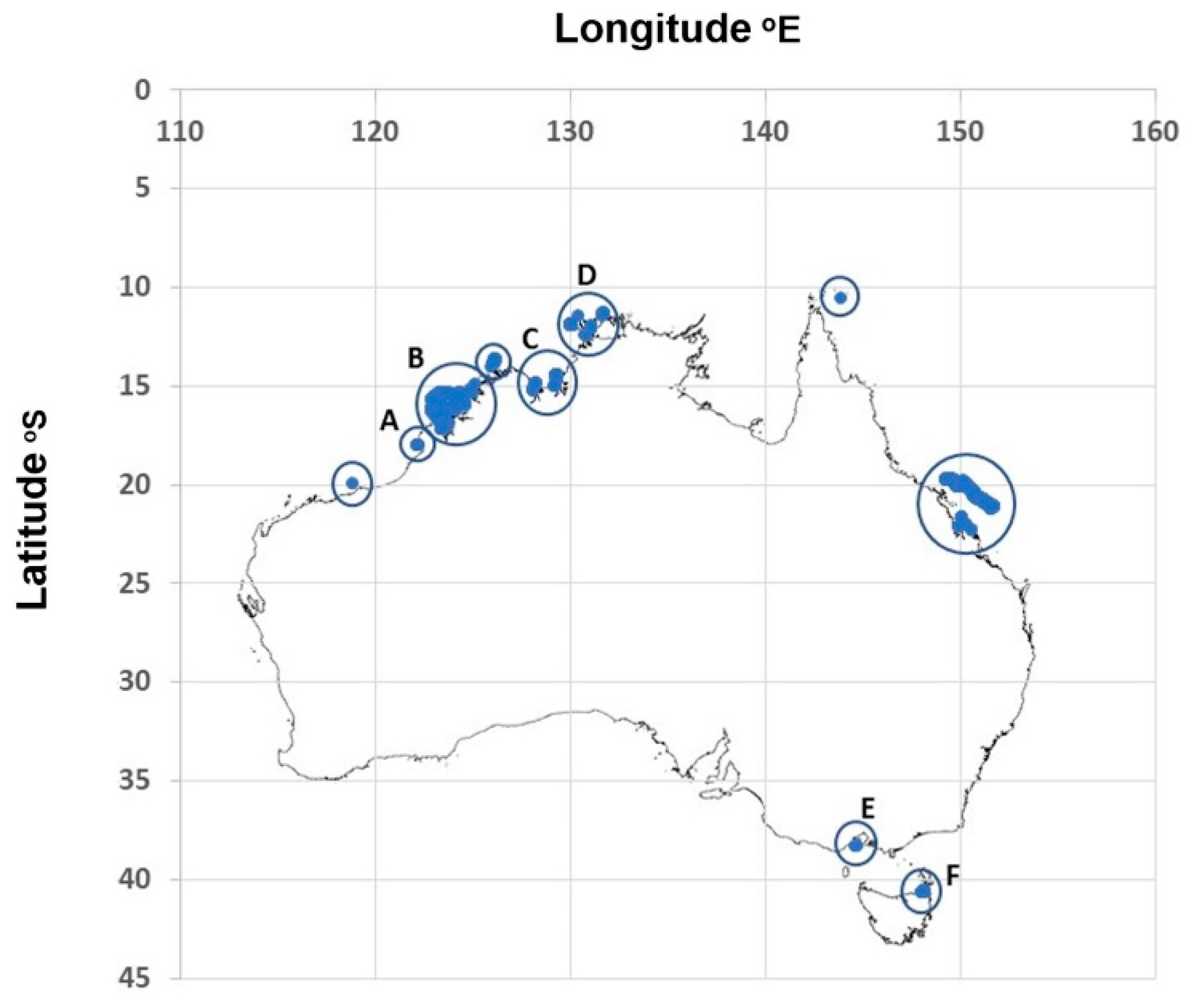
Figure 1.
Distribution, in Australia, of tidal flow rates greater than 1.5 m/s. Adapted from Tidal Energy in Australia, by Penesis et al. 2020. Copyright UTAS 2020. Adapted with permission.
Figure 1.
Distribution, in Australia, of tidal flow rates greater than 1.5 m/s. Adapted from Tidal Energy in Australia, by Penesis et al. 2020. Copyright UTAS 2020. Adapted with permission.
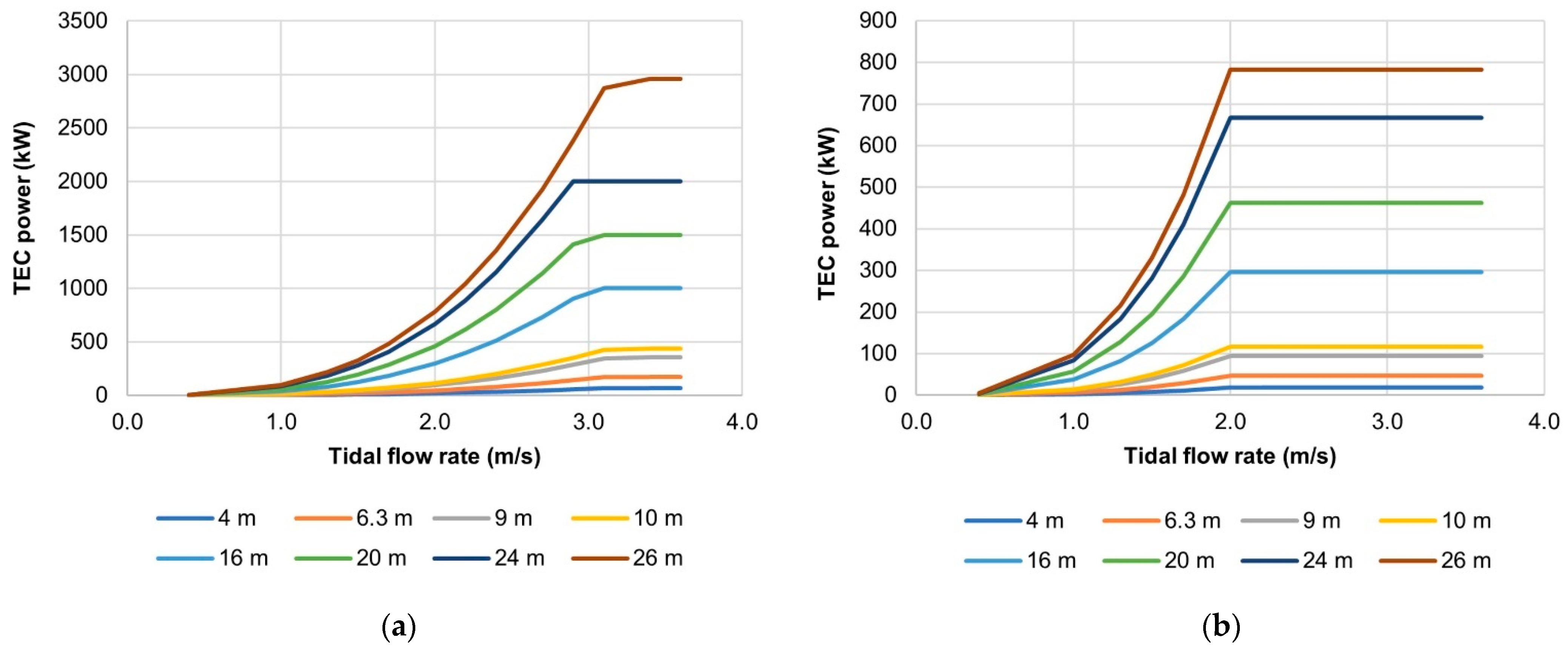
Figure 2.
Generic power curves for TEC rotor diameters ranging from 4 m to 26 m: (
a) based on commercially available TECs; (
b) matched with the Australian tidal energy resource [
6]. Copyright UTAS 2020. Adapted with permission.
Figure 2.
Generic power curves for TEC rotor diameters ranging from 4 m to 26 m: (
a) based on commercially available TECs; (
b) matched with the Australian tidal energy resource [
6]. Copyright UTAS 2020. Adapted with permission.
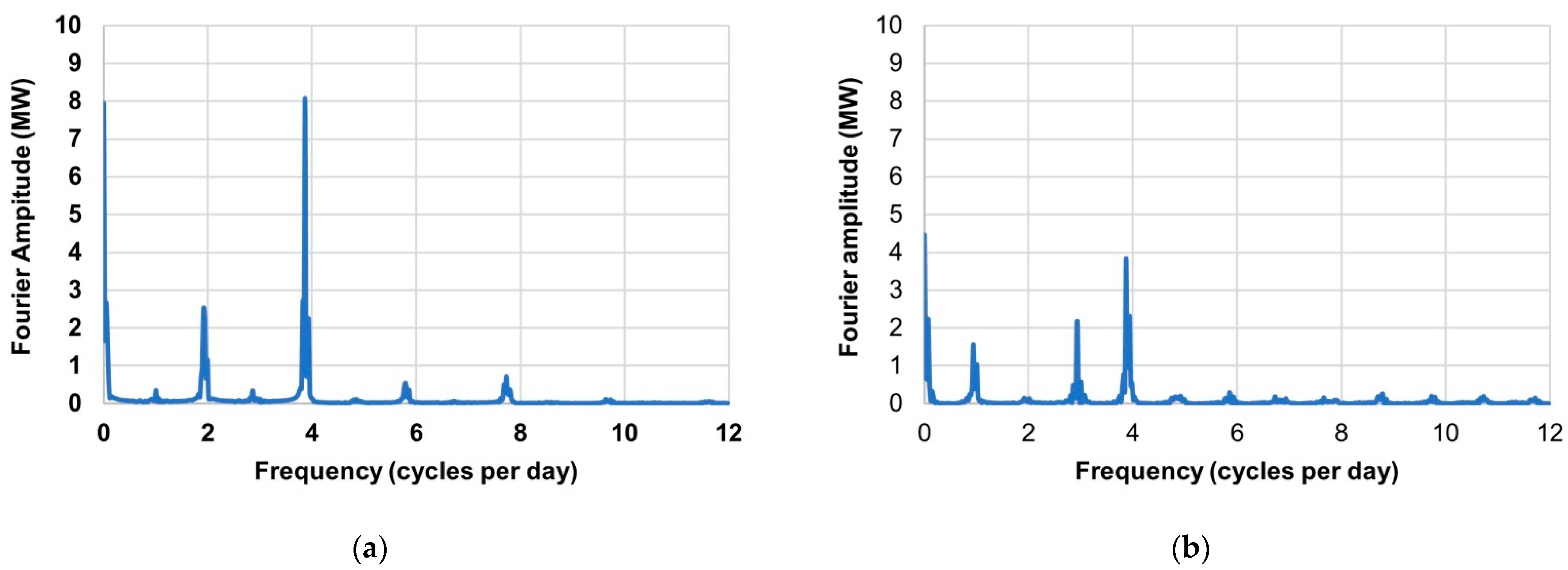
Figure 3.
FFT spectra for tidal farm hourly average electrical power samples from: (a) Banks Strait; (b) Clarence Strait. The half cycle of the period corresponding to the line at 3.9 cpd determines the low tidal power period (3.1 h) requiring battery support. The folding frequency was 12 cycles per day and the sample size was 1024 including three zero pads.
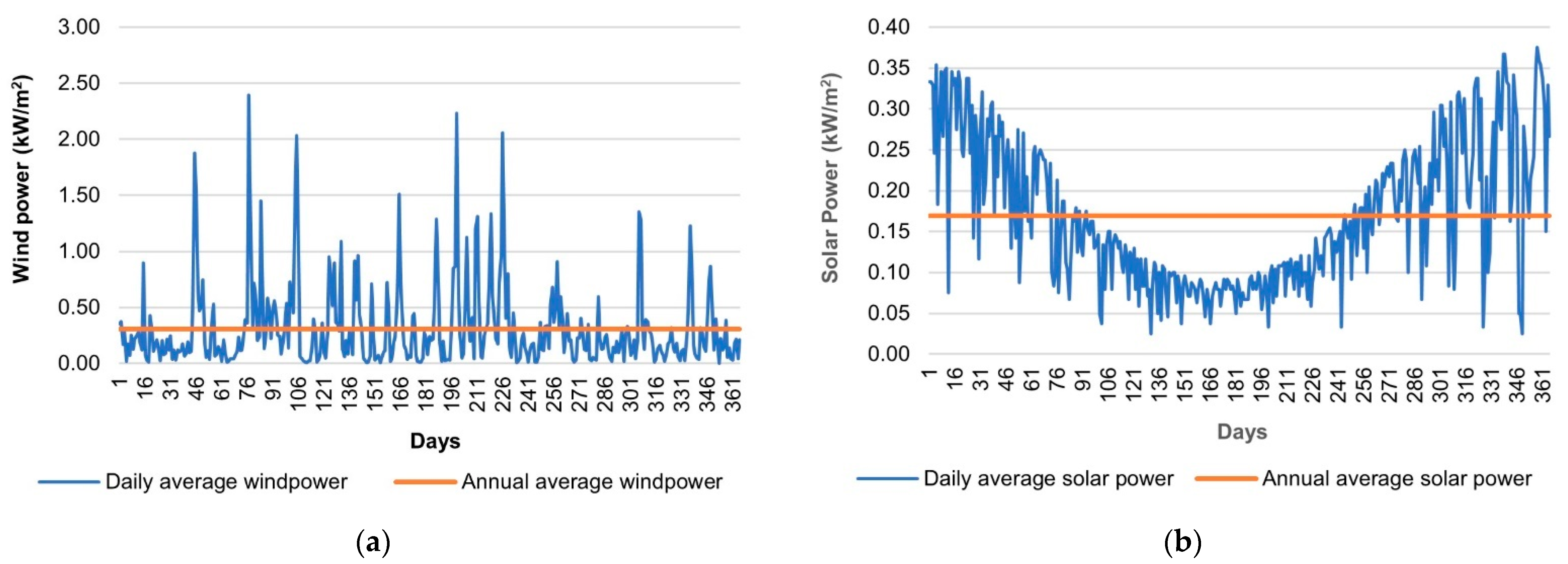
Figure 4.
Swan Island Banks Strait: (a) Wind power intermittency; (b) Solar power intermittency and variability.
Figure 4.
Swan Island Banks Strait: (a) Wind power intermittency; (b) Solar power intermittency and variability.
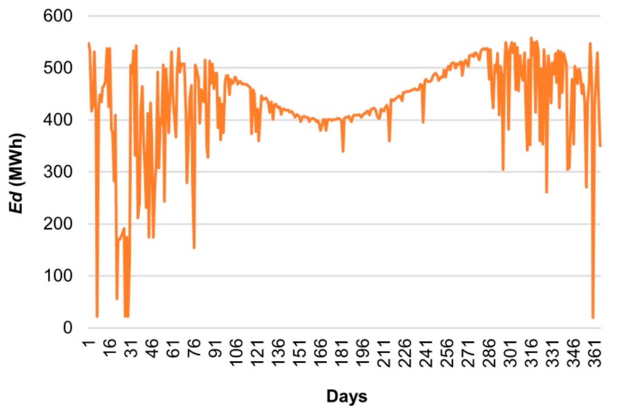
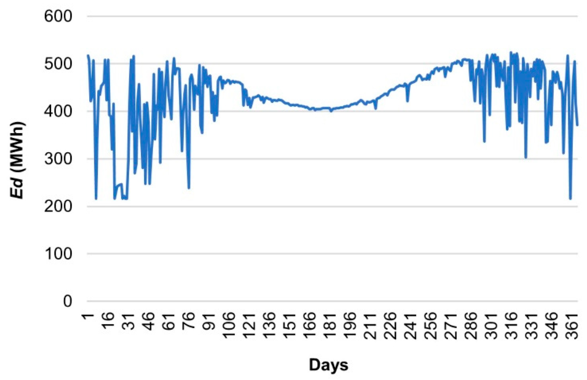
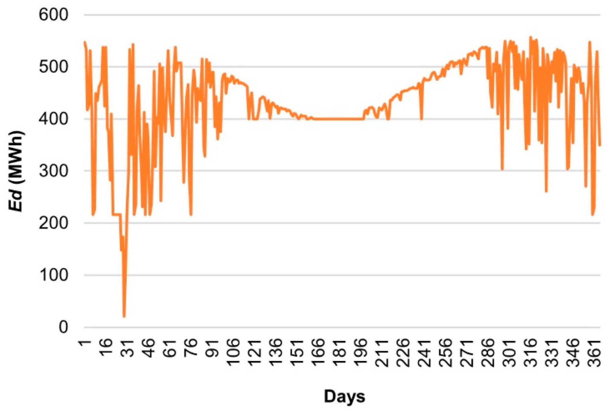
Figure 5.
Daily dispatched energy, Ed, from a solar PV farm with no energy storage and no tidal energy component. The minimum value of Ed is 21 MWh.
Figure 5.
Daily dispatched energy, Ed, from a solar PV farm with no energy storage and no tidal energy component. The minimum value of Ed is 21 MWh.
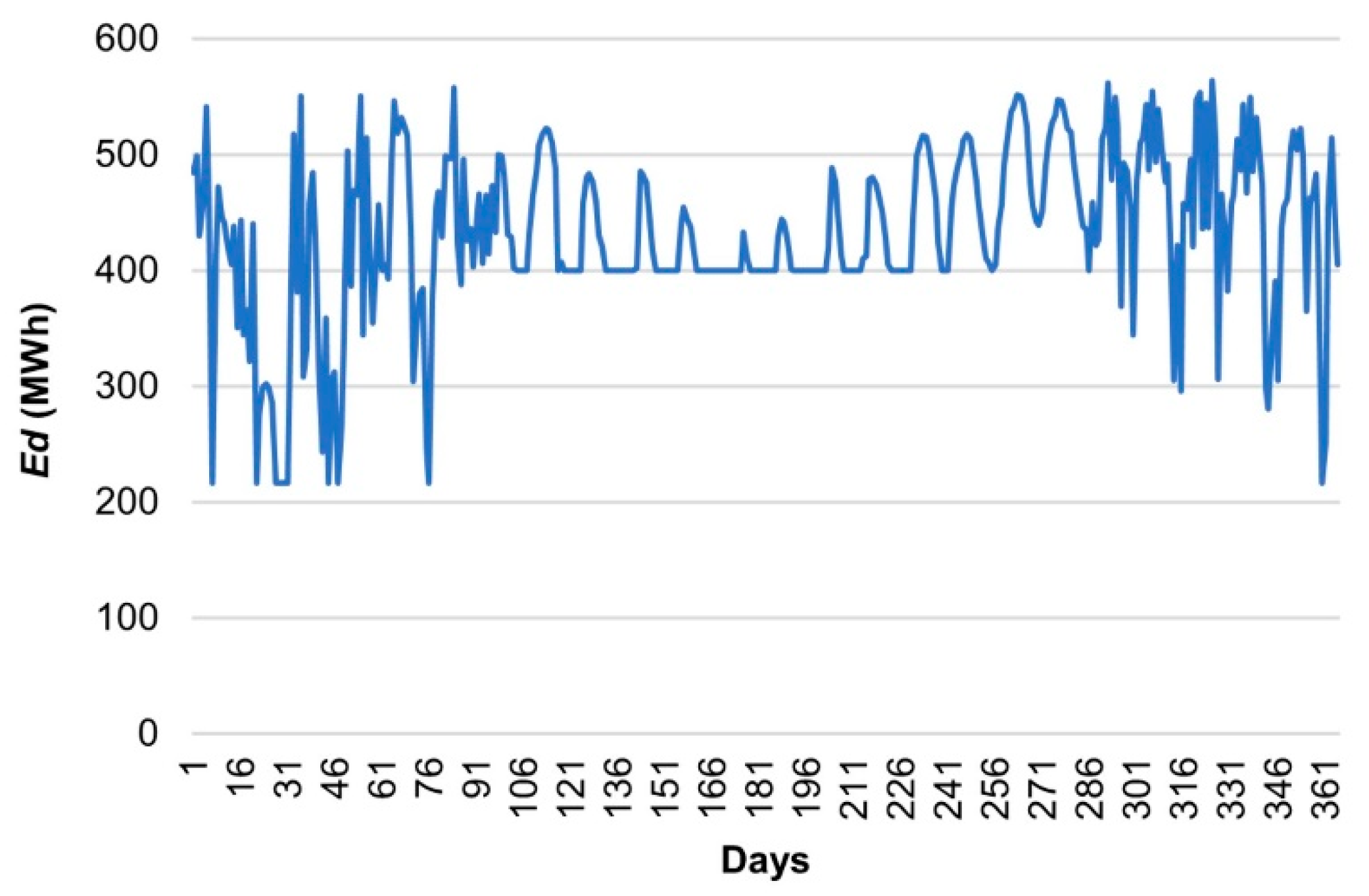
Figure 6.
Daily dispatched energy, Ed, from a tidal-solar PV farm with 624 MWh shared energy storage. The minimum value of Ed is 216 MWh, equal to Eth.
Figure 6.
Daily dispatched energy, Ed, from a tidal-solar PV farm with 624 MWh shared energy storage. The minimum value of Ed is 216 MWh, equal to Eth.
Figure 7.
Daily dispatched energy, Ed, from a tidal-solar PV farm with a 624 MWh shared battery energy capacity. The chart averages 30 tests with phase differences between the solar and tidal energy minima ranging from 0 to 29 days. The improvement in Ed exceeds or equals Eth.
Figure 7.
Daily dispatched energy, Ed, from a tidal-solar PV farm with a 624 MWh shared battery energy capacity. The chart averages 30 tests with phase differences between the solar and tidal energy minima ranging from 0 to 29 days. The improvement in Ed exceeds or equals Eth.
Figure 8.
Daily dispatched energy, Ed, from a solar PV farm with 624 MWh battery energy capacity and no tidal energy component. The minimum value of Ed is 21 MWh.
Figure 8.
Daily dispatched energy, Ed, from a solar PV farm with 624 MWh battery energy capacity and no tidal energy component. The minimum value of Ed is 21 MWh.
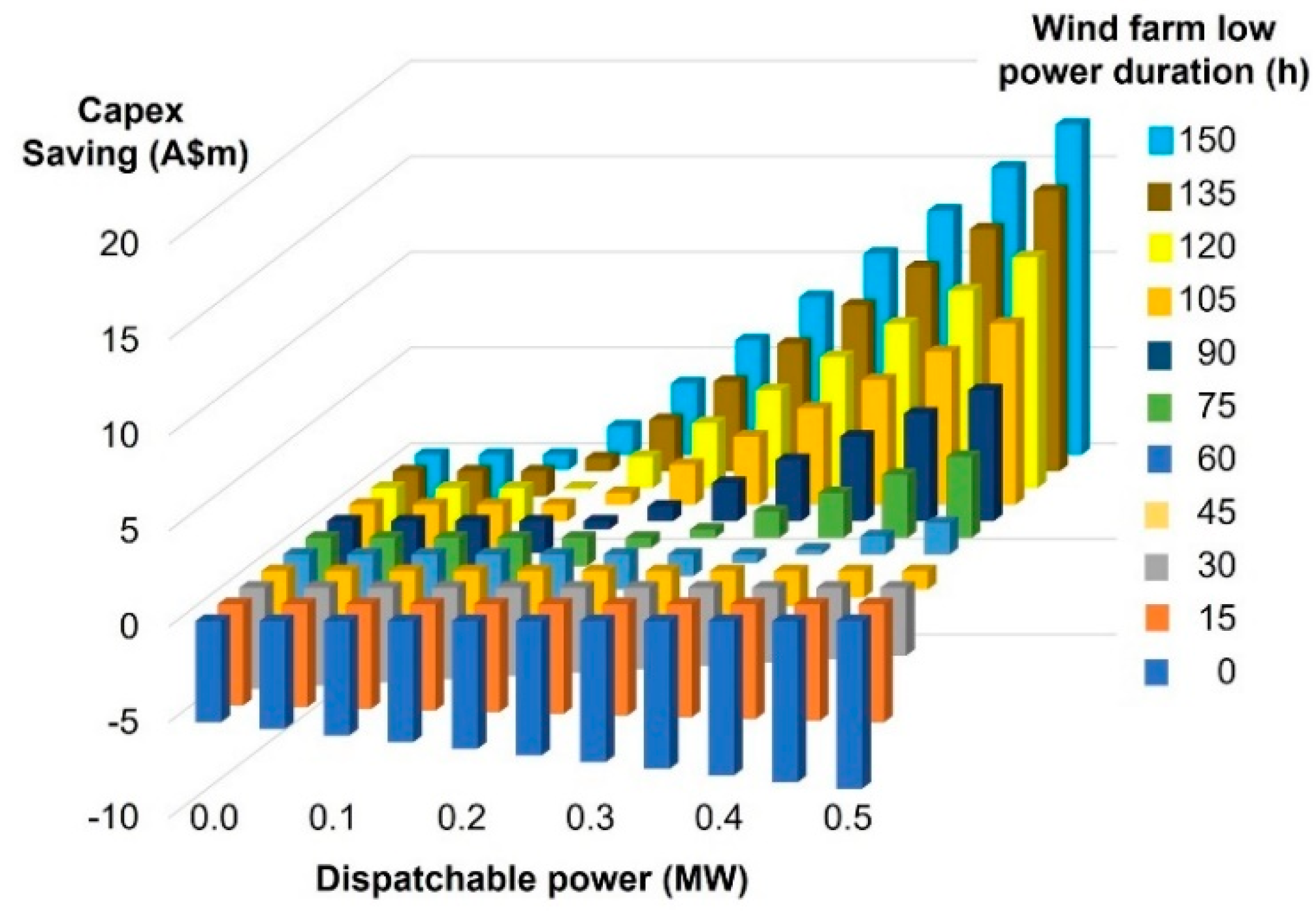
Figure 9.
The CAPEX saving dependence on the dispatchable power threshold and low power duration in a standalone offshore wind farm, (Equation (5) with: P = 1 MW, Ptidal = 0.5 × P, τtidal = 20 h, CFtidal = 0.18, CFwind = 0.45).
Figure 9.
The CAPEX saving dependence on the dispatchable power threshold and low power duration in a standalone offshore wind farm, (Equation (5) with: P = 1 MW, Ptidal = 0.5 × P, τtidal = 20 h, CFtidal = 0.18, CFwind = 0.45).
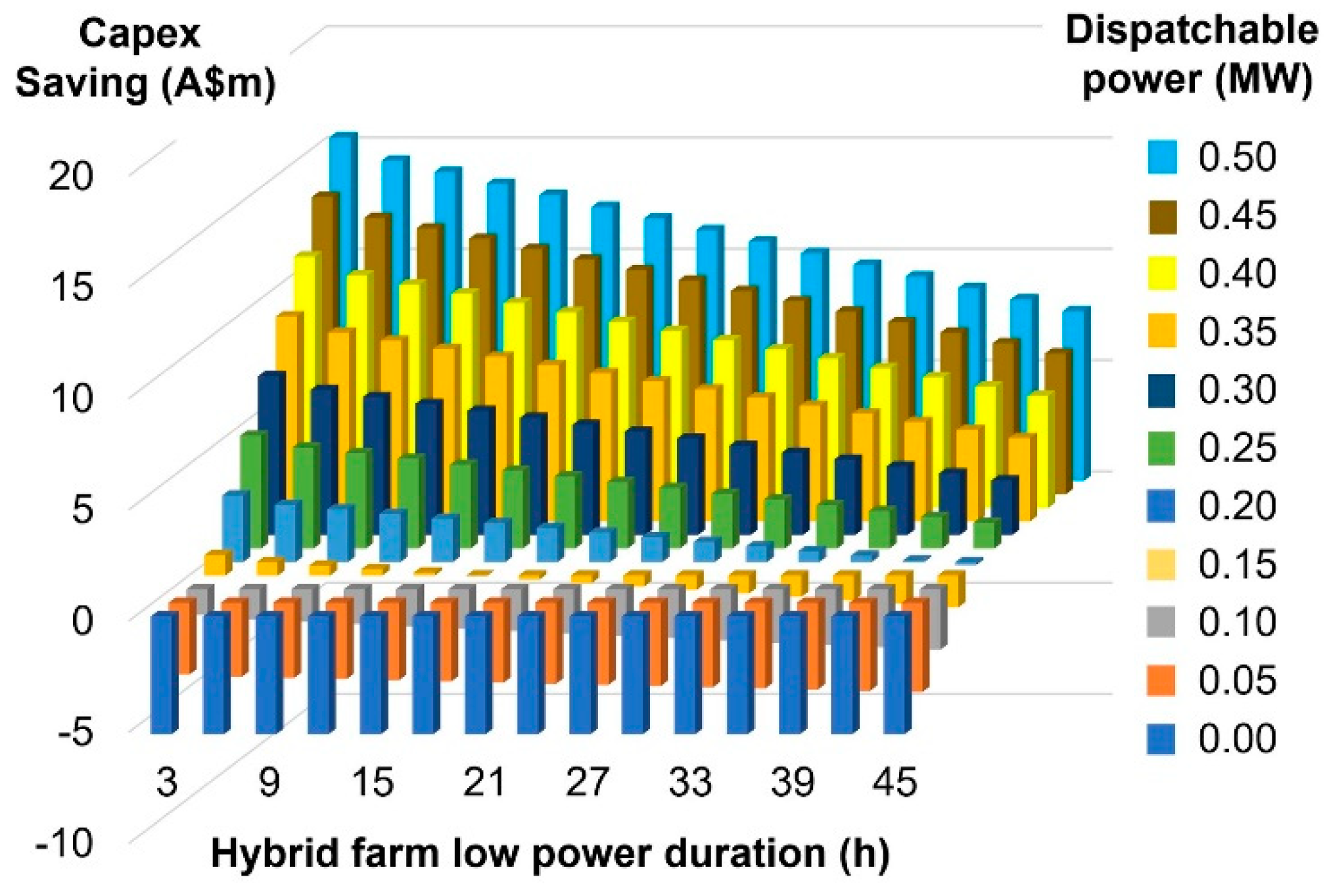
Figure 10.
The CAPEX saving dependence on dispatchable power and low power duration in a tidal-offshore wind farm. (Equation (5) with: P = 1 MW, Ptidal = 0.5 × P, τwind = 119 h, CFtidal = 0.18, CFwind = 0.45).
Figure 10.
The CAPEX saving dependence on dispatchable power and low power duration in a tidal-offshore wind farm. (Equation (5) with: P = 1 MW, Ptidal = 0.5 × P, τwind = 119 h, CFtidal = 0.18, CFwind = 0.45).
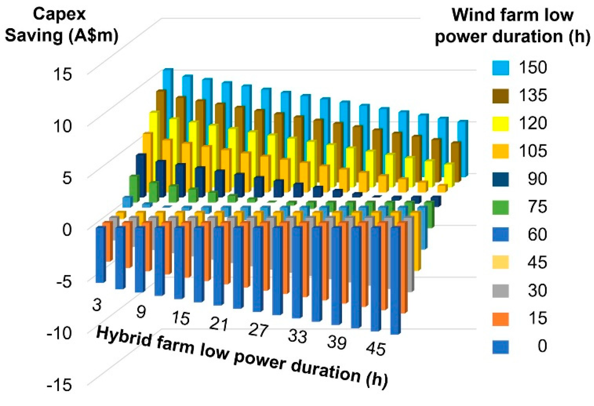
Figure 11.
The CAPEX saving dependence on low power duration in a tidal-offshore wind farm and in a stand-alone offshore wind farm. (Equation (5) with: P = 1 MW, Ptidal = 0.5 × P, Pth = 0.3 MW, CFtidal = 0.18, CFwind = 0.45).
Figure 11.
The CAPEX saving dependence on low power duration in a tidal-offshore wind farm and in a stand-alone offshore wind farm. (Equation (5) with: P = 1 MW, Ptidal = 0.5 × P, Pth = 0.3 MW, CFtidal = 0.18, CFwind = 0.45).
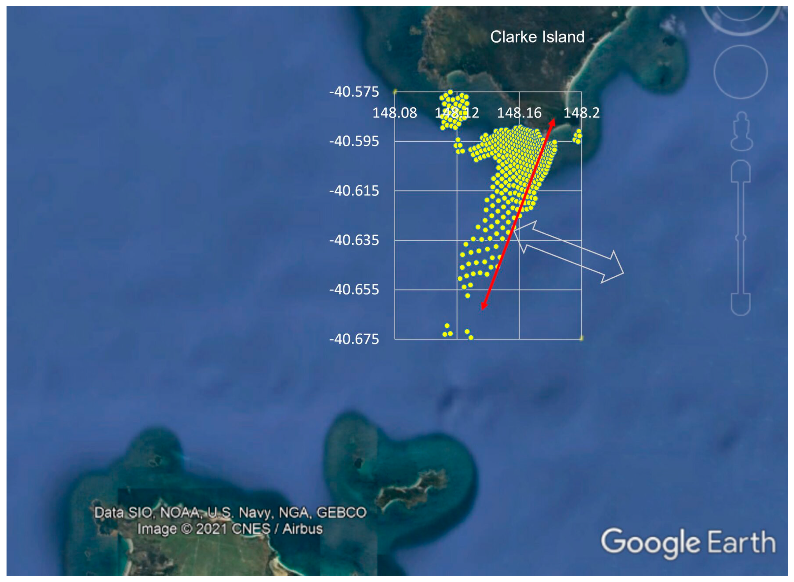
Figure 12.
Regions with a moderate to high flow rate in Northeast Banks Strait. Average tidal flow rates: 0.81 m/s, bearing 294°; 0.96 m/s, bearing 110°. The red line indicates an energy flux transect, and the grey arrow indicates an average flow direction [
20]. Data SIO, NOAA, U.S. Navy, NGA, GEBCO, Image © 2021 CNES/Airbus.
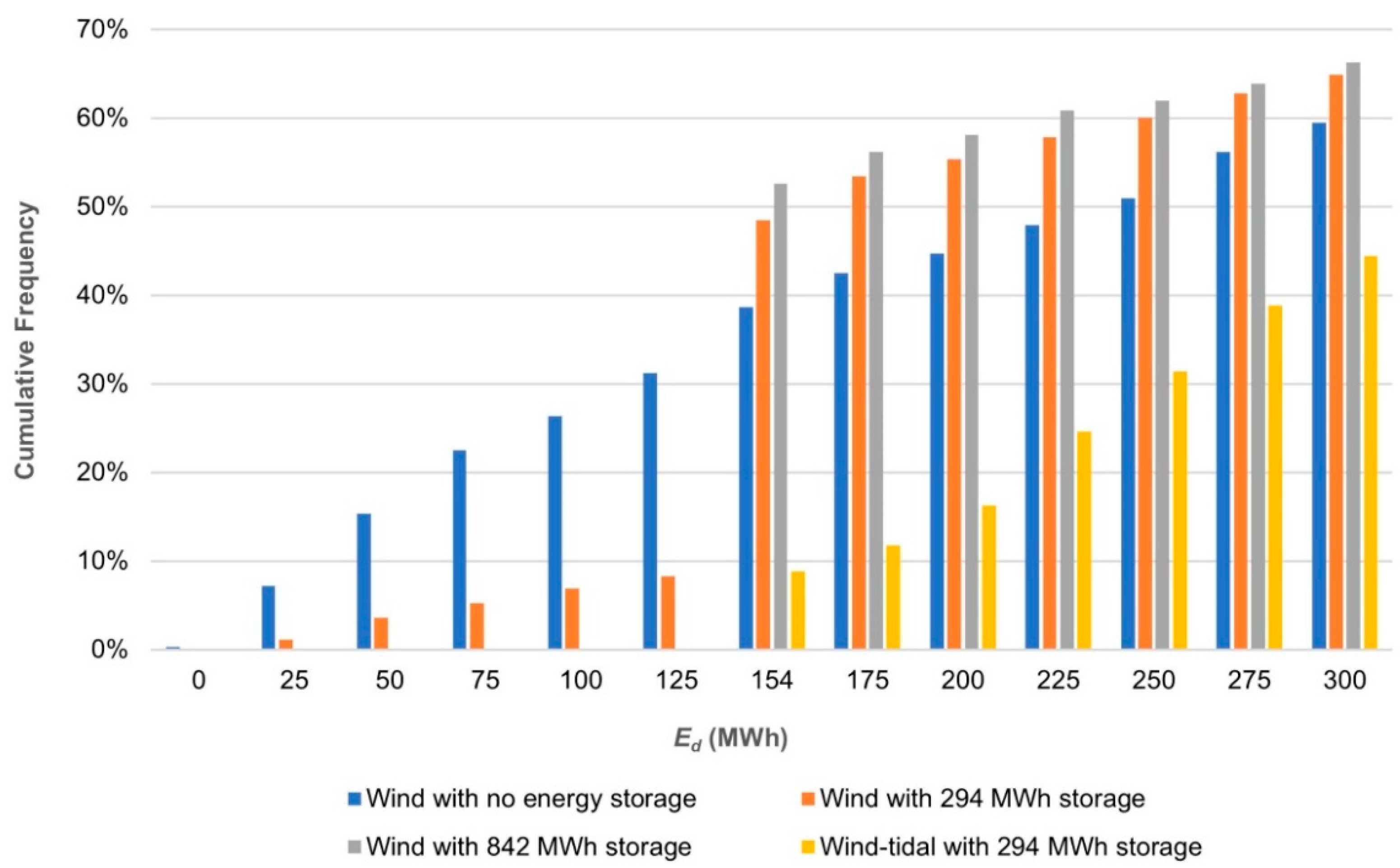
Figure 13.
Performance comparison of four configurations for a Banks Strait wind farm: (1) wind only, (2) wind with 294 MWh storage, (3) wind with 842 MWh storage, and (4) tidal and wind with 294 MWh storage. Eth is 154 MWh. In configurations 3 and 4, Ed equals or exceeds Eth (the cumulative frequency of Ed is zero below Eth). In configurations 1 and 2, Ed fails to equal or exceed Eth for 31% and 8% of the time, respectively.
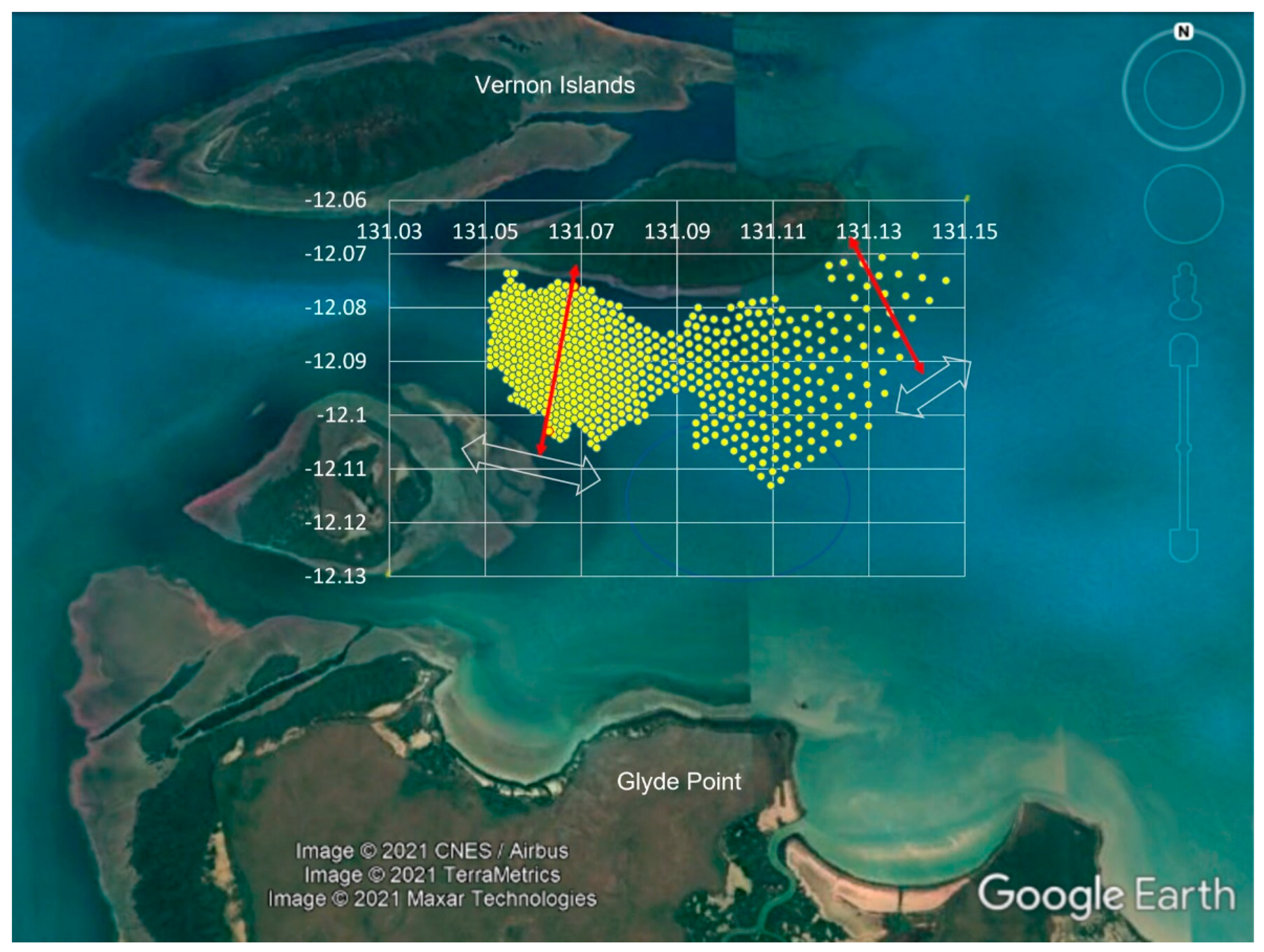
Figure 14.
Regions of moderate to high flow rate in Howard Channel. Average tidal flow rates: 1.1 m/s, bearing 286°; 0.99 m/s, bearing 102°. The red line indicates an energy flux transect, and the grey arrow indicates an average flow direction [
21]. Image © 2021 CNES/Airbus. Image © 2021 TerraMetrics. Image © 2021 Maxar Technologies.
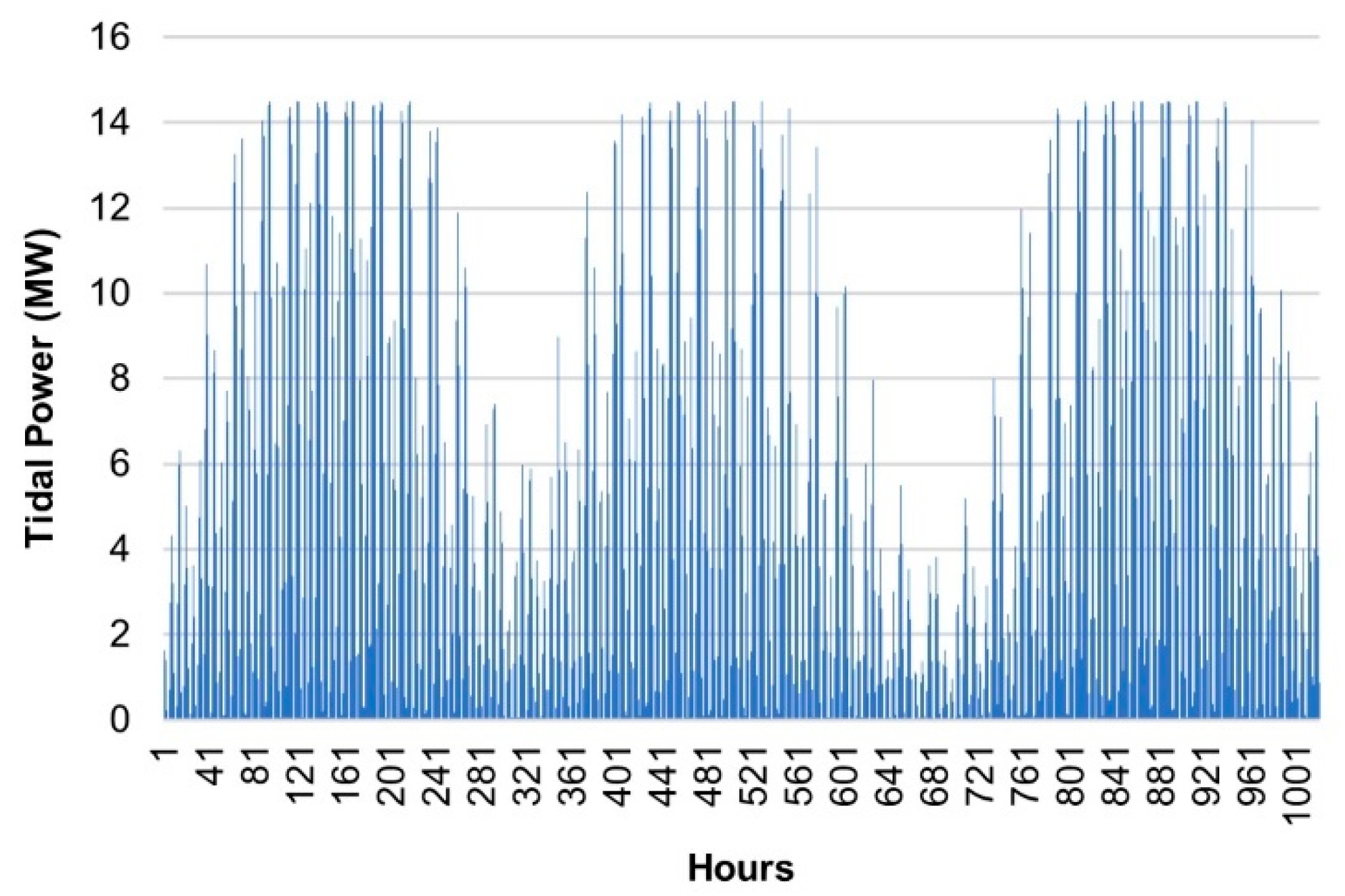
Figure 15.
Hourly average tidal power generation in Howard Channel using TECs with reduced rated power (uncropped).
Figure 15.
Hourly average tidal power generation in Howard Channel using TECs with reduced rated power (uncropped).
Figure 16.
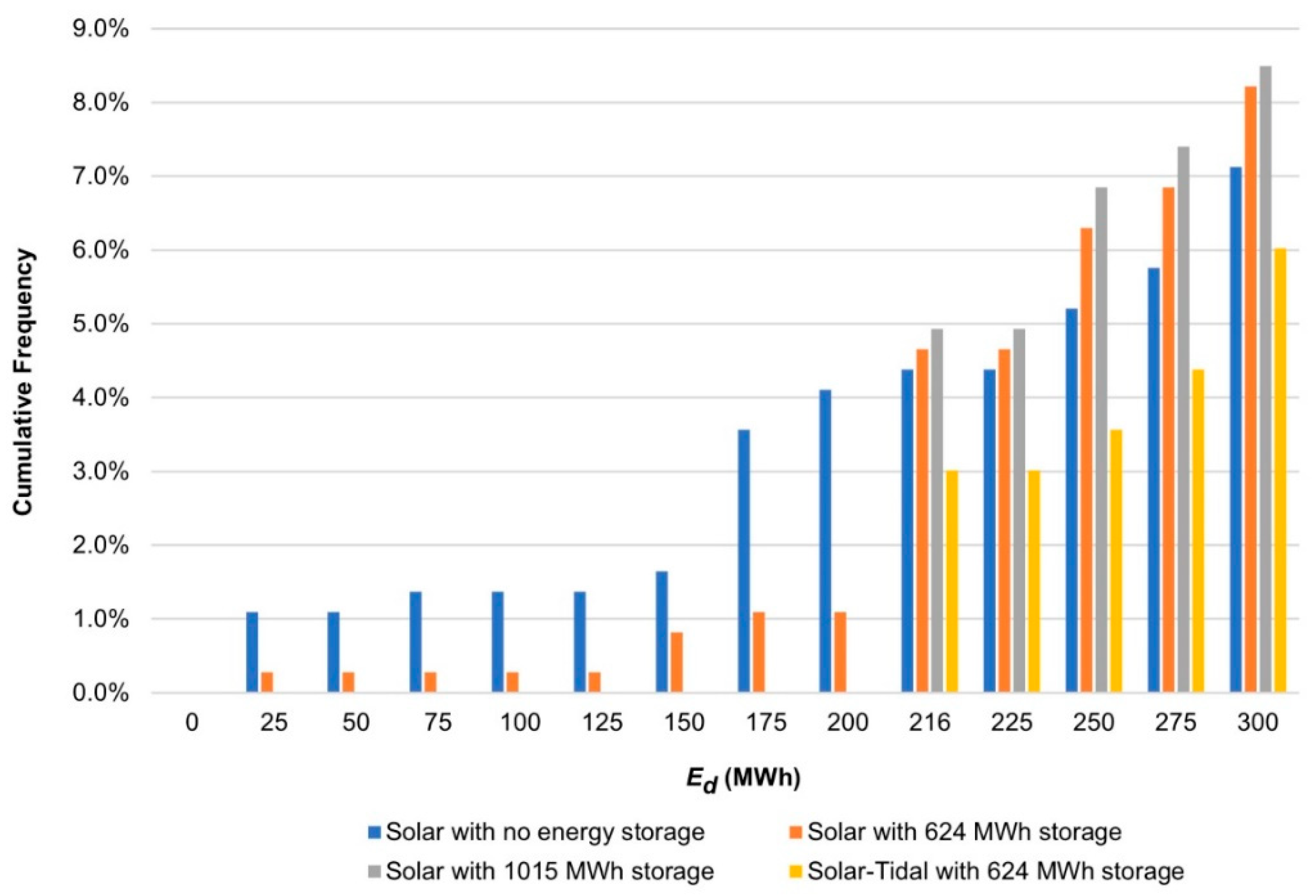
Performance comparison of four configurations for a Clarence Strait solar PV farm: (1) Solar PV only, (2) Solar PV with 624 MWh storage, (3) Solar PV with 1015 MWh storage, and (4) Solar PV and tidal hybrid with 624 MWh storage. Eth is 216 MWh. In configurations 3 and 4, Ed equals or exceeds Eth (the cumulative frequency of Ed is zero below Eth). In configurations 1 and 2, Ed fails to equal or exceed Eth for 4.1% and 1.1% of the time, respectively.
Figure 16.
Performance comparison of four configurations for a Clarence Strait solar PV farm: (1) Solar PV only, (2) Solar PV with 624 MWh storage, (3) Solar PV with 1015 MWh storage, and (4) Solar PV and tidal hybrid with 624 MWh storage. Eth is 216 MWh. In configurations 3 and 4, Ed equals or exceeds Eth (the cumulative frequency of Ed is zero below Eth). In configurations 1 and 2, Ed fails to equal or exceed Eth for 4.1% and 1.1% of the time, respectively.
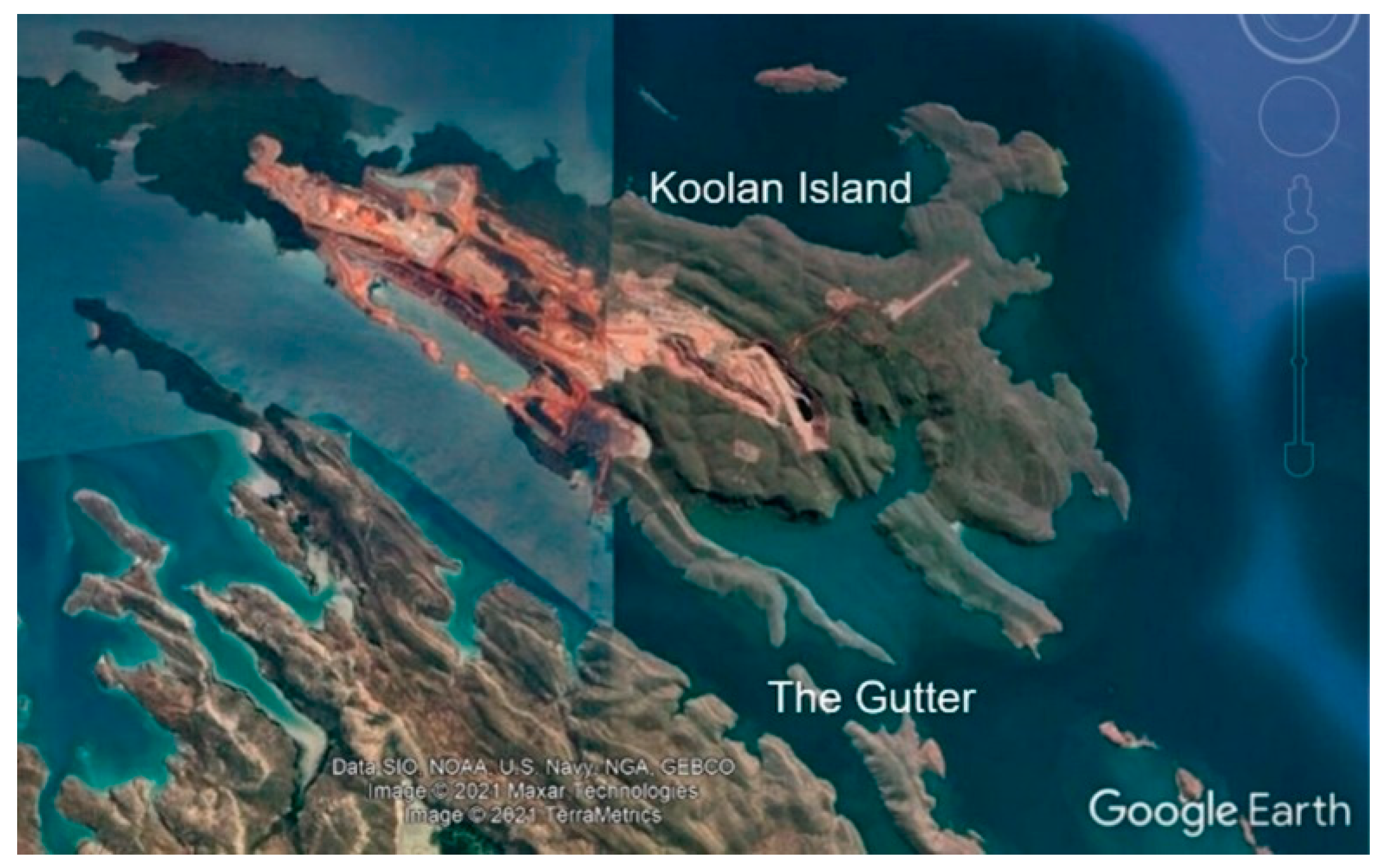
Figure 17.
Koolan Island mine site. Data SIO, NOAA, U.S. Navy, NGA, GEBCO, Image © 2021 Maxar Technologies, Image © 2021 TerraMetrics.
Figure 17.
Koolan Island mine site. Data SIO, NOAA, U.S. Navy, NGA, GEBCO, Image © 2021 Maxar Technologies, Image © 2021 TerraMetrics.
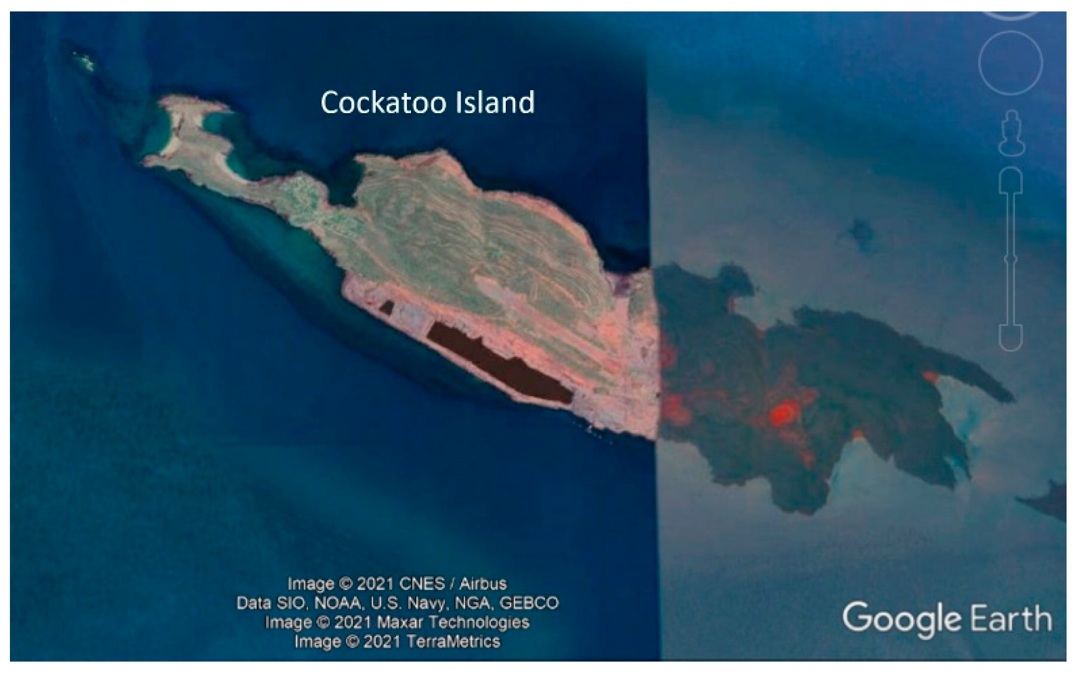
Figure 18.
Cockatoo Island mine site. Image ©2020 CNES/Airbus, Data SIO, NOAA, U.S. Navy, NGA, GEBCO, Image © 2021 Maxar Technologies, Image © 2021 TerraMetrics.
Figure 18.
Cockatoo Island mine site. Image ©2020 CNES/Airbus, Data SIO, NOAA, U.S. Navy, NGA, GEBCO, Image © 2021 Maxar Technologies, Image © 2021 TerraMetrics.
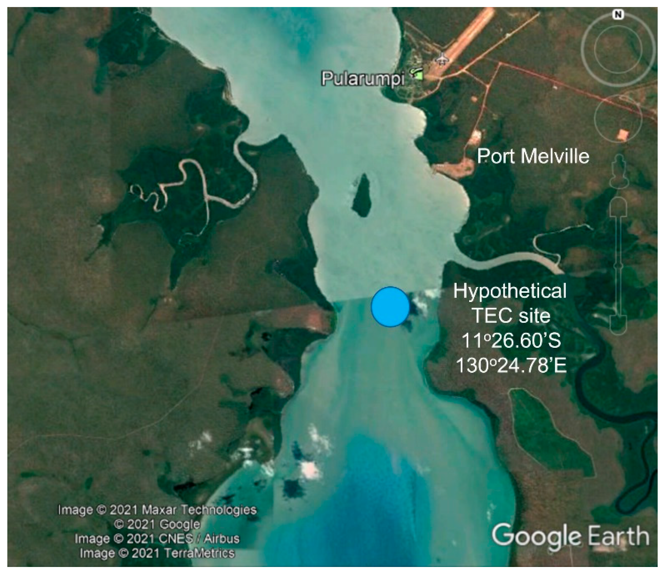
Figure 19.
Potential TEC site southwest of Port Melville, Apsley Strait. Image © 2021 Maxar Technologies, © 2021 Google, Image © 2021, CNES/Airbus, Image © 2021 TerraMetrics.
Figure 19.
Potential TEC site southwest of Port Melville, Apsley Strait. Image © 2021 Maxar Technologies, © 2021 Google, Image © 2021, CNES/Airbus, Image © 2021 TerraMetrics.
Table 1.
Renewable energy generator CAPEX values (Australia).
Table 1.
Renewable energy generator CAPEX values (Australia).
| Generator Type | 2019 (A$/kW) | 2025 (A$/kW) |
|---|
| Solar PV | 1463 | 874 |
| Offshore based, seabed attached, wind turbine | 6070 | 5424 |
| Land-based wind turbine | 1908 | 1908 |
| Tidal (modified) | 4697 | 4076 |
Table 2.
Australian sites with significant extractable tidal stream energy.
Table 2.
Australian sites with significant extractable tidal stream energy.
| Site | Capacity Factor (%) | Annual Energy
Generation (GWh) | Rated Peak Power (MW) |
|---|
| Low-resolution site assessments | | | |
| Broome [A] | 10 to 30 | 5 to 16 | 6 |
| Ardyaloon [B] | 38 | 662 | 199 |
| Derby (south beach) [B] | 17 | 40 | 27 |
| Wadeye and Tharramurr [C] | 18 | 68 | 43 |
| Port Phillip Bay [E] | 17 | 3 | 2 |
| High-resolution site assessments | | | |
| Dundas Strait [D] | 20 | 329 | 188 |
| Clarence Strait [D] | 28 | 76 | 31 |
| Banks Strait [F] | 17 | 165 | 111 |
Table 3.
Energy storage option costs CAPEX (2025).
Table 3.
Energy storage option costs CAPEX (2025).
| Energy Storage Mode | $Ebattery (A$/kWh) | $Pbattery (A$/kW) |
|---|
| Lithium batteries (2 × 10 year life) | 792 | 425 |
| Vanadium redox flow battery (20 year life) | 347 | 2810 |
| Pumped hydro (100 MW, 6 h, 100 m head) | - | 5108 |
Table 4.
Specifications for an offshore wind farm in Banks Strait with and without tidal energy.
Table 4.
Specifications for an offshore wind farm in Banks Strait with and without tidal energy.
| Specification Parameter | Wind Farm with No Tidal Energy | Wind and Tidal Hybrid Farm | Hybrid Farm
Tidal Component | Hybrid Farm
wind Component |
|---|
| Number of turbines | ~5 | ~60 | 57 | ~3 |
| Rated power (MW) | 36 | 62 | 44 | 18 |
| Capacity Factor (%) | 45 | 26 | 18 | 45 |
| Average power (MW) | 16 | 16 | 8 | 8 |
| Energy per annum (GWh) | 140 | 140 | 70 | 70 |
| Dispatchable power (MW) | 6.4 | 6.4 | 4 | 2.4 |
| Daily dispatched energy (MWh) | 154 | 154 | 96 | 58 |
| Dispatchability (%) | 40 | 40 | 50 | 30 |
| Battery energy capacity (MWh) | 842 | 294 | 24 | 270 |
Table 5.
Comparison of CAPEX (2025) for an offshore wind farm in Banks Strait with and without tidal energy.
Table 5.
Comparison of CAPEX (2025) for an offshore wind farm in Banks Strait with and without tidal energy.
| Capital Cost without Tidal Energy | A$m | Capital Cost with Tidal Energy | A$m |
|---|
| Wind turbines (36 MW) | 193 | Wind turbines (18 MW) | 97 |
| Battery (842 MWh) | 310 | Tidal turbines (44 MW) | 181 |
| Subsea cables (33 km) | 33 | Battery (294 MWh) | 120 |
| | | Subsea cables (33 km) | 33 |
| Total | 536 | Total | 431 |
Table 6.
Specification for a land-based wind farm in Banks Strait with and without tidal energy.
Table 6.
Specification for a land-based wind farm in Banks Strait with and without tidal energy.
| Specification Parameter | Wind Farm with No Tidal Energy | Wind and Tidal Hybrid Farm | Hybrid Farm
Tidal Component | Hybrid Farm
wind Component |
|---|
| Number of turbines | ~15 | ~65 | 57 | ~8 |
| Rated power (MW) | 46 | 67 | 44 | 23 |
| Capacity Factor (%) | 35 | 24 | 18 | 35 |
| Average power (MW) | 16 | 16 | 8 | 8 |
Table 7.
Comparison of CAPEX (2025) for a land-based wind farm in Banks Strait with and without tidal energy.
Table 7.
Comparison of CAPEX (2025) for a land-based wind farm in Banks Strait with and without tidal energy.
| Capital Cost without Tidal Energy | A$m | Capital Cost with Tidal Energy | A$m |
|---|
| Wind turbines (46 MW) | 87 | Wind turbines (23 MW) | 44 |
| Battery (842 MWh) | 311 | Tidal turbines (44 MW) | 181 |
| | | Battery (294 MWh) | 120 |
| | | Subsea power cables (10 km) | 10 |
| Total | 398 | Total | 355 |
Table 8.
Specifications for a solar PV farm in Clarence Strait with and without tidal energy.
Table 8.
Specifications for a solar PV farm in Clarence Strait with and without tidal energy.
| Specification Parameter | Solar PV Farm
No Tidal Energy | Solar PV and Tidal Hybrid Farm | Hybrid Farm
Tidal Component | Hybrid Farm
Solar PV Component |
|---|
| RE farm area (km2) | 0.8 | 1.1 | 0.5 | 0.6 |
| Rated power (MW) | 82 | 76 | 15 | 61 |
| Capacity Factor (%) | 22 | 24 | 30 | 22 |
| Average power (MW) | 18 | 18 | 4.5 | 13.5 |
| Energy per annum (GWh) | 158 | 158 | 39 | 118 |
| Dispatchable power (MW) | 9.0 | 9.0 | shared | shared |
| Daily dispatched energy (MWh) | 216 | 216 | shared | shared |
| Dispatchability (%) | 50 | 50 | shared | shared |
| Battery energy capacity (MWh) | 1015 | 624 | shared | shared |
Table 9.
Comparison of CAPEX (2025) for a solar PV farm in Clarence Strait with and without tidal energy.
Table 9.
Comparison of CAPEX (2025) for a solar PV farm in Clarence Strait with and without tidal energy.
| Capital Cost without Tidal Energy | A$m | Capital Cost with Tidal Energy | A$m |
|---|
| Solar PV farm (82 MW) | 71 | Solar PV farm (61 MW) | 54 |
| Battery (1015 MWh) | 378 | Tidal farm (19 × 0.8, 15 MW) | 61 |
| | | Battery (624 MWh) | 242 |
| | | Subsea power cable (10 km) | 10 |
| Total | 449 | Total | 367 |
Table 10.
Alternative products from the Clarence Strait tidal-solar PV farm.
Table 10.
Alternative products from the Clarence Strait tidal-solar PV farm.
| Product Quantities | Quantity | Value |
|---|
| Generated electricity per year [12] | 158 GWh | 8.01 A$m/year |
| Equivalent hydrogen [41,42] | 3667 t/year | 7.33 A$m/year |
| Avoided CO2-e (e-fuel from waste CO2) [36,43,44] | 20,751 t/year | 1.24 A$m/year |
| Liquid e-diesel [36,45] | 8830 t/year | 11.56 A$m/year |
Table 11.
Koolan Island and Cockatoo Island tidal farm specification options.
Table 11.
Koolan Island and Cockatoo Island tidal farm specification options.
| Location Options | Option 1 | Option 2 | Option 3 | Option 4 |
|---|
| Rotor diameter (m) | 26 | 10 | 4 | 26 |
| Number of TECs | 1 | 4 | 8 | 6 |
| Power per TEC (MW) (2 m/s tidal flow) | 0.78 | 0.12 | 0.07 | 0.78 |
| Tidal farm rated power (MW) | 0.78 | 0.46 | 0.56 | 4.69 |
| Capacity factor (%) | 20 | 20 | 10 | 20 |
| Average power (MW) | 0.16 | 0.09 | 0.06 | 0.94 |
| Annual electricity production (GWh) | 1.37 | 0.81 | 0.49 | 8.22 |
| Dispatchable power (Pth) (MW) | 0.08 | 0.05 | 0.03 | 0.31 |
| Dispatchability (%) | 50 | 50 | 50 | 33 |
| Battery energy capacity (MWh) | 2.35 | 1.39 | 0.84 | 9.38 |
Table 12.
CAPEX (2025) for Koolan Island and Cockatoo Island tidal farm options.
Table 12.
CAPEX (2025) for Koolan Island and Cockatoo Island tidal farm options.
| Configuration | Cost (A$m) |
|---|
| Option 1. Koolan Island north of Mullet Bay | |
| Tidal turbine (0.8 MW, 1 × 26 m rotor) | 3.4 |
| Subsea power cable (1.5 km to 5 km) | 1.5 to 5 |
| Energy storage (2.4 MWh) | 1.0 |
| Total | 5.9 to 9.4 |
| Option 2. Koolan Island south of Arbitration Cove | |
| Tidal turbines (4 × 116 kW, 10 m rotor) | 10.7 |
| Subsea power cable (1.5 km to 5 km) | 1.5 to 5 |
| Energy storage (1.4 MWh) | 0.6 |
| Total | 12.8 to 16.3 |
| Option 3. Koolan Island southeast (The Gutter) | |
| Tidal Turbine Reef (8 × 70 kW, 4 m rotor) | 8.8 |
| Power cable (4 km) | 4.0 |
| Energy storage (0.8 MWh) | 0.4 |
| Total | 13.2 |
| Option 4. Cockatoo Island northeast of North Bay | |
| Rated power (4.7 MW, 6 × 26 m rotor) | 20.6 |
| Power cable (1.5 km to 5 km) | 1.5 to 5 |
| Energy storage (9.4 MWh) | 4.1 |
| Total | 26.2 to 29.7 |
Table 13.
Port Melville, Apsley Strait tidal farm specification options.
Table 13.
Port Melville, Apsley Strait tidal farm specification options.
| Configuration | Option 1 | Option 2 | Option 3 |
|---|
| Rotor size (m) | 26 | 10 | 4 |
| Number of TECs | 1 | 4 | 8 |
| Rated power per TEC (kw, 2 m/s tidal flow) | 782 | 116 | 70 |
| Tidal farm rated power (MW) | 0.78 | 0.46 | 0.56 |
| Capacity factor (%) | 10 | 10 | 10 |
| Average power (MW) | 0.08 | 0.05 | 0.06 |
| Annual electricity production (GWh) | 0.69 | 0.41 | 0.49 |
| Dispatchable power (Pth) (MW) | 0.04 | 0.02 | 0.03 |
| Dispatchability (%) | 50 | 50 | 50 |
| Battery energy capacity (MWh) | 1.11 | 0.66 | 0.80 |
Table 14.
CAPEX (2025) for Port Melville, Apsley Strait tidal farm options.
Table 14.
CAPEX (2025) for Port Melville, Apsley Strait tidal farm options.
| Configuration | Cost (A$m) |
|---|
| Option 1 | |
| Tidal turbines (1 × 782 kW, 26 m rotor) | 3.4 |
| Power cable (5 km) | 5.0 |
| Energy storage (1.1 MWh) | 0.5 |
| Total | 8.9 |
| Option 2 | |
| Tidal turbines (4 × 0.116 MW, 10 m rotor) | 10.7 |
| Power cable (5 km) | 5.0 |
| Energy storage (0.66 MWh) | 0.3 |
| Total | 16.0 |
| Option 3 | |
| Tidal Turbine Reef (8 × 70 kW, 4 m rotor) | 8.8 |
| Power cable (1.5 km to 5 km) | 1.5 to 5.0 |
| Energy storage (0.8 MWh) | 0.36 |
| Total | 10.7 to 14.2 |
Table 15.
Comparison of tidal-wind and tidal-solar farms.
Table 15.
Comparison of tidal-wind and tidal-solar farms.
| RE Farm Type | Annual Energy Production | Dispatchability | Energy
Storage Mode | Battery Capacity | CAPEX Saving |
|---|
Offshore
Tidal-Wind | 140 GWh | 40% | Independent | 294 MWh | A$105m |
| Tidal-Solar | 158 GWH | 50% | Shared | 624 MWh | A$83m |


 ,
, 


