A Simplified Modeling Approach of Floating Offshore Wind Turbines for Dynamic Simulations

Abstract

Currently, floating offshore wind is experiencing rapid development towards a commercial scale. However, the research to design new control strategies requires numerical models of low computational cost accounting for the most relevant dynamics. In this paper, a reduced linear time-domain model is presented and validated. The model represents the main floating offshore wind turbine dynamics with four planar degrees of freedom: surge, heave, pitch, first tower fore-aft deflection, and rotor speed to account for rotor dynamics. The model relies on multibody and modal theories to develop the equation of motion. Aerodynamic loads are calculated using the wind turbine power performance curves obtained in a preprocessing step. Hydrodynamic loads are precomputed using a panel code solver and the mooring forces are obtained using a look-up table for different system displacements. Without any adjustment, the model accurately predicts the system motions for coupled stochastic wind–wave conditions when it is compared against OpenFAST, with errors below 10% for all the considered load cases. The largest errors occur due to the transient effects during the simulation runtime. The model aims to be used in the early design stages as a dynamic simulation tool in time and frequency domains to validate preliminary designs. Moreover, it could also be used as a control design model due to its simplicity and low modeling order.

1. Introduction

In recent decades, wind energy production growth has pushed renewable energies to directly compete with fuel-based energies [1]. In order to continue rising, the wind energy market leverages the advantages of offshore locations where the wind resource is preferable, with higher and steadier winds. In 2019, offshore wind energy capacity installation reached a peak [2], which is expected to be surpassed shortly, supported by floating wind energy development. Different commercial projects have been deployed in this direction such as Hywind Atlantic and Kincardine projects [3]. Despite the increasing amount of investment in floating solutions, the capital costs of installing a floating offshore wind turbine (FOWT) make the production costs per unit generated still high [1]. However, a viable levelized cost of energy (LCOE) reduction path could be through the implementation and testing of appropriate control strategies.

A FOWT is a highly complex nonlinear system whose representation requires considering hydrodynamics, aerodynamics, structural dynamics, mooring dynamics, controller dynamics, and their couplings. The FOWT system modeling requirements are conditioned by the design stage. The detail and accuracy needed for the model will differ from the conceptual design stage to the pre-industrial stage.

Detailed mathematical models of FOWT, including complex aerodynamics, hydrodynamics, mooring dynamics, and system structural dynamics, have been developed, allowing complex aero-hydrodynamic load representation and its influence on the system through high-fidelity time-domain simulations [4,5]. There are different software packages available to represent in detail these complex systems [6] that serve as analysis tools for system dynamics, turbine loads, fatigue damage, and cost assessment in the final design stages. In [7], a recent review of the FOWT dynamics and modeling approaches is presented. However, the most extended simulation tool for wind turbine design, both onshore and offshore, is the software named OpenFAST [8].

Although reliable FOWT modeling tools are available, which are generally based on very detailed and complex mathematical descriptions, it is of interest to develop simpler models that accurately represent the main FOWT dynamics. These simplified models can be used to: provide a clear understanding of the main system dynamics, easily modify the model parameters to check different system configurations, design controllers, and quickly test both system designs and controllers in early design stages. In the same way, these models can be helpful for scale prototype test activities. In [9,10], reduced-order models are presented for time-domain simulations. A similar model is described in [11] for dynamic performance evaluation, but simulated in the frequency domain. This low-order modeling approach is also being developed for scale prototype activities such as in [12], where the model is used for a hybrid hardware-in-the-loop test. A similar model derivation is proposed in [13], where the authors validate the model against a scaled prototype.

In general, the FOWT control research field trends towards designing controllers able to lead with more than one objective at the same time, which is basic for these systems where platform stabilization and power production are competing for wind turbine operation above rated wind [14]. A review of the current control strategies applied to different FOWT concepts can be found in [15]. The model typology for multivariable control design requires representing the system dynamics with the minimum number of variables. The control design is usually performed in a final stage through a sequential design approach [16]. However, the complexity level needed to assess control influence on global loads and motions is low, allowing modeling of the system with the dominant system dynamics considering only a few degrees of freedom [17], enabling the use of simplified models. In [18], a simplified dynamic model for control development is presented and then utilized for its purpose in, for example, [19]. A similar control-oriented model is proposed in [20] which is used to design a robust controller after being validated with OpenFAST.

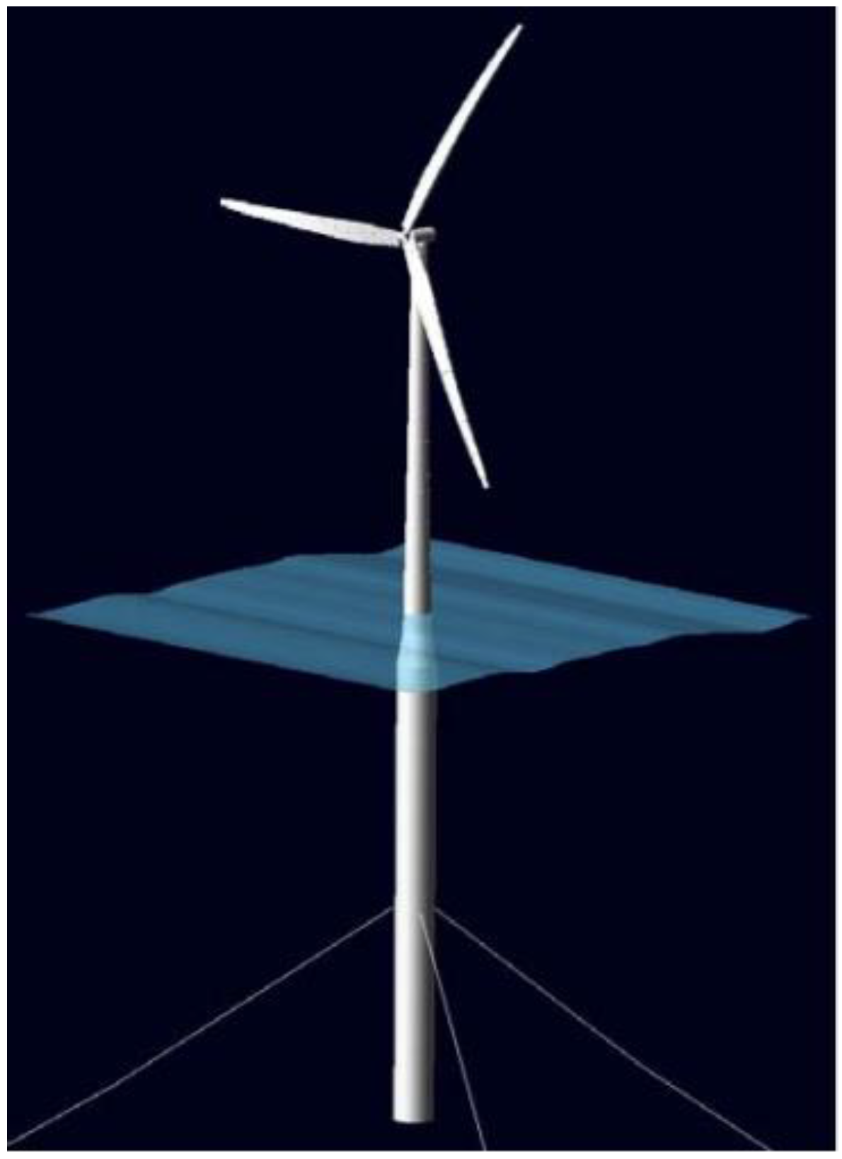
In this paper, a simplified mathematical model is proposed. The developed model is simple and represents the system dynamics well enough to be used for advanced controller design. The model’s architecture is thought to allow changing between FOWT concepts by changing the inputs to the system. The mathematical expression of the model is obtained considering the FOWT system as two rigid solids: rotor–nacelle assembly (RNA) and substructure linked by a flexible beam representing the tower. Using a 5 MW wind turbine atop a spar substructure, aerodynamic and hydrodynamic loads acting on the system are explained. A comparison of the presented model against OpenFAST is performed to validate the system dynamic response both in time and frequency domains.

The paper is structured as follows. In Section 2, the FOWT case study definition is given, defining those properties needed to build the model. Through Section 3, the modeling approach is introduced, explaining the aerodynamic, hydrodynamic, and structural dynamic representation used in the model. Section 4 summarizes the load cases and the comparison of the proposed model performance against the state-of-the-art model OpenFAST. Finally, in Section 5, some conclusions are drawn considering the results from the previous section, and possible future research directions are also mentioned in this last section.

2. Case Study

The presented model is validated using the OC3 Hywind Spar buoy shown in Figure 1 as a case study. The floating system’s main properties including the platform, the wind turbine, and the mooring system are summarized based on the description provided in [21].

The platform hull reaches 10 m above sea water level (SWL) and has a draft of 120 m. The stability of this floating platform concept is achieved by a restoring moment generated by the difference in height between the mass and buoyancy centers. In

Table 1. OC3 Hywind platform properties [21].

Parameter	Value	Units
Depth to platform base below SWL (Draft)	120	m
Elevation to platform top above SWL	10	m
Taper top depth below SWL	4	m
Taper bottom depth below SWL	12	m
Platform diameter above the taper	6.5	m
Platform diameter below the taper	9.4	m
Platform mass	7,466,330.0	kg
Platform center mass (CM) below SWL	89.9155	m
Platform pitch inertia about CM	4,229,230,000	kg m2
Additional linear damping ($B_{11}^{linear}$)	100,000	N s m−1
Additional linear damping ($B_{33}^{linear}$)	130,000	N s m−1

, the main properties used for the development of the reduced model are summarized.

The wind turbine modelled is the NREL5MW [22], which is a variable-speed variable-pitch (VSVP) controlled turbine often used as a reference turbine for research purposes. The hub height of the onshore turbine is 90 m above ground, so the tower height of the model is shortened to match the same hub height of the onshore turbine due to the platform hull height above water level. Tower top and bottom diameters are unchanged. The wind turbine properties are shown in

Table 2. OC3 Hywind wind turbine properties [22].

Parameter	Value	Units
Rated power	5	MW
Rotor diameter	126	m
Hub height	90	m
Rotor mass	110,000	kg
Rotor inertia	35,444,067	kg m2
Generator inertia	534.116	kg m2
Generator friction	16.5489	N s/m
Gearbox ratio (high-speed to low-speed)	97	-
Nacelle mass	240,000	kg
Nacelle CM above tower top	1.96	m
Tower mass	347,460	kg

.

The mooring system properties are described in [21] and summarized in

Table 3. OC3 Hywind mooring system properties [21].

Parameter	Value	Units
Unstretched mooring line length	902.2	m
Mooring line diameter	0.09	m
Equivalent mooring line mass density	77.7066	kg/m
Equivalent mooring line weight in water	698.094	N/m
Equivalent mooring line extensional stiffness (EA)	384,243,000	N

. It consists of three catenary lines attached to the platform via delta connection. In the model, this configuration is simplified to reduce the system complexity as was done in the OC3 project. The fairleads are located at 70 m below SWL and symmetrically spread at a 5.2 m radius from the platform centerline, mounting a mooring system configuration where lines are 120° separated. Anchors are fixed at a radius of 853.87 m from the platform centerline and at a depth of 320 m.

3. Modeling Approach

As it is explained in [23], a control-oriented wind turbine model is usually derived using the Multibody System approach (MBS). With this technique, reduced low-order models can be obtained allowing the consideration of only those degrees of freedom that are directly coupled to the controller actions. In a variable-speed variable-pitch (VSVP) wind turbine operation, the speed control interacts with the modes in the rotation frame such as drivetrain torsion mode and blade edgewise bending modes. However, these modes’ natural frequencies fall beyond the controller bandwidth frequency [23], allowing the simplification. The pitch control not only affects the power production through the aerodynamic torque but also changes the thrust excitation force. In consequence, tower bending mode and floating system rigid solid modes, affected by the thrust excitation force, should also be considered.

In the present work, a planar MBS is derived, presenting the FOWT as two lumped masses, platform, and rotor nacelle assembly (RNA), connected by a flexible tower. The model describes the FOWT dynamics attending to the interaction between the rotor and the along-wind modes. Surge, heave, and pitch rigid-body modes are considered in the model since they are identified as the most critical modes for FOWT control design [24], with the pitch mode a limitation for traditional control strategies [25,26]. The first fore–aft tower modal deflection is also included because it is significantly excited by aerodynamic forces due to its low natural frequency. These loads can be reduced using the blade pitch control for wind speeds above the rated value [27] and, consequently, a lighter tower and foundation could be designed. Finally, the rotor dynamics are also represented by a single degree of freedom equation of motion.

The time-domain equation of motion is based on Newton’s second law:

$$\left[M\right]\left\{\ddot{x}\left(t\right)\right\}+\left[C\right]\left\{\dot{x}\left(t\right)\right\}+\left[K\right]\left\{x\left(t\right)\right\}=\left\{F_{Ext}\left(t\right)\right\}$$

(1)

where the motion vector $\left\{x\left(t\right)\right\}$ comprises the motions in each of the considered degrees of freedom (DOF). $\left[M\right]$, $\left[C\right]$, and $\left[K\right]$ are, respectively, the mass, damping, and stiffness matrices of the system. All the previously introduced matrices are 5 × 5 according to the represented system motions. The system total mass sums the contribution of the structural mass and the hydrodynamic added mass from the inertial component of the radiation force. The damping matrix is mounted from the contribution of three damping terms. First, the linear hydrodynamic damping is presented before in the case study section. The second is the structural damping of the system. Thirdly, the damping contribution from the radiation force is added to the model through direct integration of the convolution of the product between radiation impulse response and the state velocity. Finally, the contribution from the hydrostatic restoring and structural stiffness are included in the system stiffness matrix. The last term, $\left\{F_{Ext}\left(t\right)\right\}$, represents the external forces acting on each of the system DOFs. In the present model, this load vector encompasses wind $\left\{F_a\right\}$, wave $\left\{F_h\right\}$, excitation forces, and mooring loads $\left\{F_{moor}\right\}$. In Figure 2, a block diagram of the proposed FOWT model is presented:

In the following subsections, the different terms of the previously presented dynamic equation are obtained for the case study model.

3.1. Aerodynamics

The interaction between the wind and the turbine is defined by the aerodynamic model. Commonly, the Blade Element Momentum (BEM) theory is applied to define the wind turbine aerodynamic loads [28]. This theory is a complex computational method that requires iterations to obtain the axial and tangential induction factors needed to calculate the lift and drag forces in each of the blade sections. The use of this theory is avoided during simulation runtime due to the numerical effort required for induction coefficient determination. However, it is applied in a pre-processing stage where the wind turbine aerodynamic properties are obtained using Aerodyn [29] for different rotor speeds and pitch angles assuming nacelle motions are small so the aerodynamic properties remain constant. These properties, power coefficient, $C_P\left(\lambda , \beta \right)$, and thrust coefficient, $C_T\left(\lambda , \beta \right)$, shown in Figure 3, are computed as functions of the blade pitch angle and the tip speed ratio (TSR or $\lambda$), which is the relation between the blade tip linear speed and the incident wind:

$$\lambda =\frac{\Omega R}{v_w}$$

(2)

In the present model, the wind turbine aerodynamics are written based on the non-dimensional power and thrust coefficients represented as:

$$F_a=\frac{1}{2}· {\rho }_{air}·A_{Rotor}·C_T\left(\lambda , \beta \right)·v_{Rel}^2$$

(3)

$$M_a=\frac{1}{2}· {\rho }_{air}·A_{Rotor}·\frac{C_P\left(\lambda , \beta \right)}{\Omega }·v_{Rel}^3$$

(4)

where ${\rho }_{air}$ is the air density, $A_{Rotor}$ is the rotor area, $\Omega$ is the rotor speed, and $v_{Rel}$ is the relative wind speed at hub height, calculated as the wind speed ($v_w$) reduced by the hub velocity ($v_{hub}$):

$$v_{Rel}=v_w-v_{hub}$$

(5)

3.2. Structural Dynamics

Floating wind turbine motions and structural responses are consequence of rigid-body motions rather than elastic deformations [30]. Hence, rigid-body theory is accurate enough to represent the FOWT dynamics for control design. However, the proposed model is augmented to a multi-body elastic deformation model to consider the tower as a flexible element due to the influence of the wind excitation force into the tower dynamics and controller design. The tower is a continuous structure that can be discretized in various ways. If shear deformation and lateral inertia effects are neglected, the tower deformation can be modelled with a generalized displacement in combination with the principle of virtual displacements, as is proposed in [31] and later used to model a FOWT in [11,32]. In the proposed model, this theory is followed to describe the tower response. The mode is described by a shape function; thus, the accuracy of the modelled response depends on how well the deformation is captured by the shape function. These shape functions are commonly chosen to be the most relevant eigenmodes of the system. In this case, it is the tower’s first fore-aft bending mode. In the proposed model, the tower bending mode shape function is obtained using BModes [33].

Three rigid-body modes of motion and one flexible mode are considered in the model, namely, surge, heave, pitch, and the first tower fore-aft bending mode, respectively. Motions are referenced to the center of gravity of the whole system. The tower mode introduces off-diagonal terms in the system matrixes to couple the bending mode with surge and pitch modes. The actual bending mode shape needed to represent the tower fore-aft mode is not known and is, therefore, obtained from an eigenvalue solution. Consequently, it is assumed that the shape of the fore-aft mode is kept in the coupled model.

An additional variable is added to represent the rotor dynamics. Assuming a rigid drivetrain, a first-order dynamic equation is applied to consider the rotational speed of the rotor in the proposed model:

$$\left(I_R-r_T·I_g\right)·\dot{\Omega }=\left(M_a-r_T·M_g\right)$$

(6)

where the overall drivetrain inertia is computed by the rotor inertia ($I_R$) and the generator inertia ($I_g$) expressed in the low-speed shaft by the gearbox relation ($r_T$). The inertia is balanced by the aerodynamic torque ($M_a$) and the generator torque ($M_g$), which is kept constant to obtain the required rotor speed ($\Omega$).

3.3. Hydrodynamics

In a spar-type foundation, one of the most widely used methods is related to the Morison equation and strip theory [34]. The theory is applied for a certain environmental condition where waves are large, and the floating structure is considered slender. Since the presented model aims to be used for control strategy design, which is assessed within the wind turbine operational range, the environmental sea conditions are smoother, enabling solution of the radiation–diffraction problem with the linear potential flow theory [35,36]. The frequency-dependent added mass and radiation damping are precomputed in panel code software, such as the programs AQWA [37] or WAMIT [38], for the specific OC3 platform shape. The hydrostatic restoring matrix including the contribution from the buoyancy center (CB) and waterplane area together with the wave excitation force are obtained from the panel code solver based on the previously mentioned linear potential flow theory.

To compute the time-domain hydrodynamic radiation force, the sum of added mass and radiation damping, the so-called free-surface memory effect, is considered by the convolution integral of the retardation function. In [39,40], the approach based on the potential theory results is developed and validated. The time-domain values for the added mass and radiation damping are computed as follows:

$$A_{\infty }=a\left(\omega \right)+{{\displaystyle \int }}_0^{\infty }B\left(\tau \right)·\sin \left(\omega \tau \right)\mathrm{dt}$$

(7)

$$B\left(\tau \right)=\frac{2}{\pi }·{{\displaystyle \int }}_0^{\infty }b\left(\omega \right)·\cos \left(\omega \tau \right)\mathrm{d}\mathsf{\omega }$$

(8)

where $a\left(\omega \right)$ is the added mass and $b\left(\omega \right)$ is the radiation damping, both function of frequency. $B\left(\tau \right)$ is the retardation function obtained from the cosine transformation of the impulse radiation function. Additionally, the hydrodynamic damping model is augmented with additional linear damping, which is added to match the free-decay test, as is detailed in [21] and summarized in Table 1. Second-order effects would be of significant influence in surge motions and need to be accounted for to conclude the benefits of specific control strategies. However, this aspect falls beyond the scope of this paper and has not been introduced. Slowly varying second-order drift forces will be considered in subsequent versions of the presented model, enabling its applicability to assess wind turbine control strategies.

3.4. Mooring Dynamics

The floating system is anchored to the seabed by three catenary mooring lines, with a delta connection to increase the stiffness in yaw. However, the simplifications assumed in [21] are also considered. Each of the mooring lines is supposed as a continuous cable with homogeneous properties. If the forces from inertia, viscous drag, internal damping, and bending and torsion modes are neglected, a quasi-static analysis approach can be applied to obtain the non-linear catenary stiffness as a function of the platform movement, as is justified in [41]. In a preprocessing step, the mooring stiffness forces are obtained for different platform displacements that are then used as a look-up table to compute the forces in each simulation time step.

3.5. Modeling of Wind and Wave Resource

Wind and wave modeling is simulated following the guidelines provided in [42]. The Kaimal spectrum model is selected to include the turbulent component of the wind and the JONSWAP spectrum is used to represent different sea states. The wind speed Kaimal spectrum is defined by the following expression:

$$S_k\left(f\right)={\sigma }_U^2\frac{6.868\frac{L_U}{U_{10}}}{{\left(1+10.32\frac{f L_U}{U_{10}}\right)}^{5/3}}$$

(9)

In this expression, $f$ denotes the frequency, ${\sigma }_U$ is the wind standard deviation, $U_{10}$ is the 10 min mean wind speed at 10 m height above the still water level, and $L_U$ is the integral length scale of the wind speed process. This last parameter can be obtained as:

$$L_U=300 {\left(\frac{z}{300}\right)}^{0.46+0.074\ln z_0}$$

(10)

where $z$ is the height above sea water level and $z_0$ is the terrain roughness calculated by:

$$z_0=\frac{A_c}{g} {\left(\frac{k_{a}U\left(z\right)}{\ln \left(\frac{z}{z_0}\right)}\right)}^2$$

(11)

where $k_a$ is the von Karman’s constant ($k_a=0.4$), $g$ is the gravity acceleration, and $A_c$ is the Charnock’s constant, which is dependent on the wave velocity and the available water fetch. The definition of the implemented method for $A_c$ is given in [43]. The simulations carried out in Section 4 are computed using the turbulent wind speed time series developed with the proposed model; see Figure 4.

The waves are modelled following the Airy wave theory, which considers that the fluid layer has a uniform depth and its flow is inviscid, incompressible, and irrotational [39]. The JONSWAP wave spectrum is utilized due to its validity to represent a sea state in a fetch limited situation, and it is formulated by:

$$S_j\left(\omega \right)=A_{\gamma }{S}_{PM}\left(\omega \right) {\gamma }^{\exp \left(-0.5\left(\frac{\omega -{\omega }_p}{\sigma {\omega }_p}\right)\right)}$$

(12)

where the Pierson–Moskowitz spectrum ($S_{PM}$) is defined as:

$$S_{PM}\left(\omega \right)=\frac{5}{16} H_S^2 {\omega }_p^4 {\omega }^{-5}\exp \left(-\frac{5}{4}{\left(\frac{\omega }{{\omega }_p}\right)}^{-4}\right)$$

(13)

The parameter $H_S$ is the significant wave height, ${\omega }_p$ is the angular spectral peak frequency obtained from the peak period value ($T_p$), and $\omega$ is the angular frequency. $A_{\gamma }$ is a normalizing factor function of the non-dimensional peak shape parameter, $\gamma$, and $\sigma$ is a spectral width parameter. The values used for the parameters are those proposed in [42]. The wave elevation used in Section 4 simulations is obtained using this spectrum. In Figure 4, the irregular wave elevation time series can be seen.

4. Model Validation

The model is implemented in Python and its accuracy is tested against OpenFAST [8]. OpenFAST is a multi-physics, multi-fidelity tool for simulating the coupled dynamic response of wind turbines, both fixed and floating. The OC3 project [44] collects results from different modeling tools including OpenFAST. To validate the proposed low-order model, some of the load cases simulated in that project are used. In

Table 4. Load cases for model comparison.

Load Case	Models	Wind	Waves	Analysis
1	OpenFAST Reduced Model	None	None	Eigenanalysis Decay Tests
2	OpenFAST Reduced Model	None	Regular	RAOs
3	OpenFAST Reduced Model	None	Irregular JONSWAP spectrum $\begin{array}{c}{H}_s=6 \mathrm{m} \\ T_p=10 \mathrm{s}\end{array}$	Time series PSDs
4	OpenFAST Reduced Model	Turbulent: Kaimal spectrum $V_w=8 \mathrm{m}/\mathrm{s}$	None	Time series Statistics
5	OpenFAST Reduced Model	Turbulent: Kaimal spectrum $V_w=18 \mathrm{m}/\mathrm{s}$	Irregular: JONSWAP spectrum $\begin{array}{c}{H}_s=6 \mathrm{m} \\ T_p=10 \mathrm{s}\end{array}$	Time series PSDs Statistics

, a summary of the different load cases is shown:

In the following, the comparison of the results between the proposed model and OpenFAST is presented. All the simulations have a simulation length time of 1800 s, and to avoid initial transient effects the first 800 s are neglected. The controller dynamics are simulated for a specific operation point, which means a constant rotor speed and a constant blade pitch angle for the complete simulation. The values for the wind turbine steady operation are obtained from [22]. This is done to reduce the number of variables acting on the system’s dynamic response.

4.1. Load Case 1

The system natural frequencies are calculated with the proposed model by solving the eigenvalue problem mathematically described as:

$$\left(-\left\{{\omega }_n^2\right\}\left[M\right]+\left[K\right]\right)\left\{\widehat{x}\left(\omega \right)\right\}=\left\{0\right\}$$

(14)

To obtain the natural frequencies in OpenFAST, a PSD of the decay test revealed the system’s damped natural frequency. A comparison of natural frequencies is given in

Table 5. System natural frequency and periods comparison.

Degree of Freedom	Frequencies (Hz)		Periods (s)
	Reduced Model	OpenFAST	Reduced Model	OpenFAST
Surge	0.008	0.008	125.53	125.00
Heave	0.032	0.032	31.10	31.25
Pitch	0.034	0.034	29.63	29.41
1st tower fore–aft mode	0.498	0.472	2.01	2.12

, where it is shown that all system natural frequencies agree well with the OpenFAST identification.

To represent the system response in absence of forces, free-decay tests are carried out. To compare the results from both the proposed model and OpenFAST, the same initial conditions are given as inputs on both model simulations. In Figure 5, time-domain simulation outputs are shown for each of the DOFs. The same natural frequency error is appreciated in the decay period and a slightly lower system damping.

4.2. Load Case 2

This load case considers the solution to regular waves excitation ($F_w$) in absence of wind. To perform a comparison of the proposed model against OpenFAST, the frequency-domain solution of Equation (1) is obtained with the reduced model:

$$\left(-{\omega }^2\left[M\right]+i\omega \left[C\right]+\left[K\right]\right)\left\{x\left(\omega \right)\right\}=\left\{F_w\left(\omega \right)\right\}$$

(15)

Both OpenFAST and reduced model time-domain simulation are carried out for different regular wave periods of unit wave amplitude. Then, the simulation output maximum amplitude is plotted into the frequency-domain solution as can be seen in Figure 6.

Generally, the response to regular waves agrees well when it is compared against OpenFAST simulations. Slight differences are observed in the tower fore–aft mode frequency peak due to the limitations of the followed modeling structural approach. In the same way, a lower system damping is appreciated in low frequencies for the distinct hydrodynamic and structural properties.

4.3. Load Case 3

To compare the results, the same wave elevation series is given as input in OpenFAST and the proposed model. The solutions to the FOWT system motion are shown in Figure 7, where both time-domain series and power spectral density functions (PSDs) are illustrated.

The motion response agrees quite well for each of the DOFs considering the hydrodynamic properties difference. The time-domain series present differences due to transient effects; however, the frequency components validate the proposed model response when it is compared against OpenFAST.

4.4. Load Case 4

This load case is proposed to validate the aerodynamics of the system through an evaluation of the mean displacement,

Table 6. Mean displacement LC4.

DOF	Reduced Model	OpenFAST	Error (%)
Surge (m)	12.70	12.40	−2.41
Pitch (deg)	2.63	2.51	−4.78
Fore–aft (m)	0.23	0.22	−4.54

, and standard deviation,

Table 7. Standard deviation LC4.

DOF	Reduced Model	OpenFAST	Error (%)
Surge (m)	1.571	1.613	2.48
Pitch (deg)	0.358	0.336	−5.88
Fore–aft (m)	0.023	0.024	−3.10

. The statistics show that the proposed model response is congruent with the OpenFAST model in steady-state conditions.

As is shown in Figure 8, the motions of the proposed model and OpenFAST are similar for windspeed below rated value.

4.5. Load Case 5

The last load case tries to represent the environment where the wind turbine will operate. In Figure 4, the turbulent wind speed and the wave elevation used in this load case are shown. In

Table 8. Mean displacement LC5.

DOF	Reduced Model	OpenFAST	Error (%)
Surge (m)	10.648	10.516	−1.255
Pitch (deg)	2.185	2.149	−1.675
Fore–aft (m)	0.201	0.191	−5.235

and

Table 9. Standard deviation LC5.

DOF	Reduced Model	OpenFAST	Error (%)
Surge (m)	1.638	1.762	7.037
Pitch (deg)	0.837	0.830	−0.843
Fore–aft (m)	0.124	0.131	5.343

, the mean displacement and the standard deviation are presented, respectively.

The time series and PSDs of the coupling wind and waves simulations are presented in Figure 9.

Both obtained statistics and system motion responses present comparable results for the proposed model and OpenFAST. However, the same transient error effects are appreciated in this load case due to the differences in wave excitation force application.

4.6. Discussion

The proposed model validation against OpenFAST considering five different load cases shows a good agreement between models. The main reason to select the simulation cases is due to an increasing complexity of the selected simulation case, from simulations in absence of loads with a prescribed initial displacement to a fully coupled aero-hydro-elastic simulation with turbulent wind and irregular waves. This increasing complexity level allows to easily detect the differences between models and quantify them.

The proposed model and OpenFAST results agree well for the Decay Test and Eigenvalue problem solutions. However, slight differences can be appreciated in time-domain responses. The different periods shown in the results are a consequence of the different modeling approaches followed to model the structural dynamics of the model, namely, in the method applied to model the fore–aft DOF and the couplings between motions. Similarly, a higher damping value can be appreciated for the fore–aft displacement due to differences in the structural damping. The reason is due to the restriction applied by the modal shape function utilized to represent the tower fore–aft flexible mode.

The results from load cases 2 and 3 are used to validate and quantify the differences between the hydrodynamics. The frequency components of the responses in both load cases agree well with OpenFAST results. However, differences are detected in the response to regular waves of the fore–aft mode consequence again of the different modeling approaches followed to mathematically represent the system. The RAOs for solid rigid motions—surge, heave, and pitch—are well captured, although lower damping can be appreciated for low frequencies in pitch and tower top fore–aft displacements. These differences in low frequencies are due to the couplings between the different DOFs.

Load case 4 is used to validate the aerodynamic model used in the proposed model. The heave response is not added because the thrust aerodynamic load is horizontally applied within the model. The responses from the proposed model and OpenFAST coincide well both in time and frequency for the turbulent wind in absence of waves. However, slight differences can be observed due to the different system configuration regarding the position of the different subsystems in the global coordinate system affecting the mass distribution and stiffness of the system. Similarly, lower damping is noted due to the differences commented above. Moreover, the simplified moorings dynamics applied to the proposed model can influence the differences in the mean displacement of the whole system.

Finally, Load case 5 is considered as a final validation test where the system is simulated close to the real operation conditions applying irregular waves and turbulent wind. The results obtained from the proposed model are like those from OpenFAST. However, some transient effects can be highlighted due to the progressive application of loads in the proposed model. Regarding the system damping, it appears to be lower at the wind excitation frequency, around 0.05 rad/s, but higher around wave excitation frequency. This variation in damping, which is a consequence of the above-mentioned hydrodynamic damping difference together with the aerodynamic damping which is related to the relative wind speed seen by the rotor and with the aerodynamic properties of the reduced aerodynamic model.

5. Conclusions

In this paper, a simplified two-dimensional model for floating offshore wind turbine dynamic simulation is presented. The system is reduced to two bodies linked by a flexible beam. The mathematical expression is formed by a set of stiffness, damping, and mass matrices, which are solved together considering the FOWT as a single mechanical multi-degree-of-freedom system which is solved in time and frequency domains.

The validation of the proposed numerical FOWT model is performed for different load conditions to assess the quality of the response. In general, the differences related to the structural dynamic model and hydrodynamic properties are few and their influence in the global system response is low, with errors below 10% for all load cases. The quality in the motion response encourages use of the model as a control design tool or for control co-design methodology. Additionally, the results obtained for the spar buoy foundations motivate extending the modeling approach to other floating substructure concepts.

Future research will include new versions of the current model, including the calculation of the structural loads at the tower base and extension of the hydrodynamic model to consider the application of slow varying drift forces which influence the surge motion. These improvements will also be contrasted and validated using the OpenFAST model. Additional research will be focused on the development of new control design strategies for FOWT systems. The utilization of the proposed model will enable the design advanced control methods such as Model Predictive Control (MPC) and Linear Quadratic Regulators (LQR) which are based on the represented model states. Additionally, the consideration of the tower bending mode can enable the inclusion of new sensors into the controller to develop a control strategy that considers the tower base fatigue information to increase the system life.