Study of the Influence of Nonlinear Dynamic Loads on Elastic Modulus of Carbonate Reservoir Rocks

Abstract

The paper presents the results of the experimental investigation of carbonate reservoir rocks subjected to quasistatic and nonlinear dynamic loads. During the quasistatic loading the zones of linear elasticity were determined. Dynamic loading of samples was performed at several frequencies and load amplitudes using a testing system. There were two zones found in which the elastic modulus changes nonlinearly in terms of dynamic load frequency. While the frequency of the dynamic load increases from 0 to 10 Hz the dynamic elastic modulus rises according to logarithmic law; while the frequency increases from 10 to 60 Hz elastic modulus rises according to a power law for each load amplitude. The amplitude of the longitudinal strain and phase shift decreases with increasing frequency of the dynamic load. Under the higher strain rates the rock gets stiffer in comparison with rock subjected to smaller strain rate dynamic loading. Saturation of rock samples with distilled water flattening the dependencies of dynamic Young’s modulus on frequency.

1. Introduction

Dynamic loads are taken into account while designing concrete [1] and aerospace [2] structures, tunnels [3], deeply buried constructions [4], propulsion system of ships [5], reinforced polymer structures in civil engineering [6] and many other fields. In those fields engineers deal with mechanical characteristics of different materials such as for example metals or composites. During mining and development of hydrocarbon reservoirs the engineers are aware of the behavior of mechanical characteristics of rocks subjected to dynamic loads. In particular, during the drilling of an oil production well the engineers face the nonlinear dynamic phenomena [7] (downhole vibration) caused, for example, by bit bounce [8,9]. Such the oscillatory influence of a bit on a bottom hole rock forces its mechanical properties (e.g., stiffness) to apparently vary in dynamics, which change the bit-rock interaction and consequently the effectiveness of a drilling process [10]. On the one hand, mechanical characteristics of rocks can be decreased and rate of bit penetration into the rock can be increased using high frequency axial [11] or circular [12] bit oscillations, but on the other hand the rock can be strengthened with increasing strain rate and its dynamic mechanical characteristics can be higher that static ones [4,13]. At the same time the energy of longitudinal vibrations of a drill string can be used to increase the rock breaking efficiency [14,15]. In order to ensure a proper regime of rock fracture the change in mechanical characteristics of rocks while dynamic influence on it should be evaluated. To take into account the dynamic components of mechanical characteristics in the calculations, the engineers require to know the laws according to which those characteristics change when dynamic loads are applied. One of the most widely used characteristics of the mechanical properties of rocks used in engineering calculations are the elastic moduli, and Young’s modulus in particular. Dynamic mechanical characteristics of rocks are studied under one-way [13], multistage [16,17], cyclic [18,19] and high-frequency loading [20]. To study the dynamic mechanical characteristics using traditional testing systems or loading stands additional sensors are required. Studying of the nature of the change in the modulus of longitudinal elasticity of rocks under the influence of dynamic loads (elastic vibrations with frequency and amplitude) is limited by the complexity of research in dynamics, as well as the subsequent interpretation of the data [21]. The behavior (change) of the mechanical characteristics of rocks in dynamics is revealed during experiments using installations of the Split Hopkinson (Kolsky) Bar type [22,23], or on stands for uniaxial compression with an additionally installed oscillator. For instance, the dispersion of elastic characteristics of such sedimentary rocks as Fontainebleau sandstone and Opalinus Clay shale was revealed in experimental works [24,25] while dynamic loading using stands with an oscillator. The authors of [26] also revealed the dispersion of the elastic modulus when studying the Pierre shale at a dynamic loading stand. In a more recent work [27] the authors used an experimental setup also reviled the dispersion of the elastic moduli of sandstone and gypsum with increasing frequency. According to studies carried out in [28] on an experimental setup, Young’s modulus of a clastic rock (New red sandstone) increases from 10 to 40 Hz in accordance with a power law. However, some earlier works (see, for example, [29]) reported that Young’s moduli of Navajo sandstone, Spergen limestone and Oklahoma granite do not depend on the frequency of dynamic loading at a frequency ranging from 4 to 400 Hz. The nature of the behavior of elastic characteristics still remains not fully understood. In this regard, the purpose of the present work is to study the behavior of a longitudinal elastic modulus of a sedimentary rock subjected to dynamic loading.

Existing experimental papers on determining the behaviour of the dynamic Young’s modulus of rocks are mostly dedicated to the field of seismic survey and therefore deal with seismic frequencies at strain rates from 10⁻⁸ to 10⁻⁵ (see for example [24,25,30,31]). However, in the field of an oil well drilling at the bottom of a well the bit can bounce together with an entire heavy drill string at much higher rates. Thus, the rocks at a well bottom are subjected to much higher impact loads (vibrations) which has a negative effect on the drilling effectiveness. In order to model the conditions in our experimental work we performed dynamic loading when rock experiences dynamic strain at the strain rates of up to 10⁻³ (at the frequency equal to 60 Hz). A number of experimental paper deals with similar strain rates or even higher but those studied are one-way (not cyclic). Studies of cyclic loading of rocks is also common in this area, but those studies usually deal with low frequency range. However, we performed the nonlinear dynamic loading of a carbonate rock with a higher strain rate approaching the field conditions. Besides, another scientific contribution is that we noticed a small region of low frequencies where the dynamic Young’s modulus behaves according to a law different to commonly known.

An investigation on dynamic loading is performed on prepared rock samples in a zone of uniaxial compressive strength test diagram where stress and strain are related linearly. To determine the limits of the zone of linear elasticity on the stress-strain diagram of rock samples, quasi-static loading tests were carried out first. Then, in the zone of linear elasticity, dynamic loading tests were performed on samples with a dynamic load frequency varying from 0.1 Hz to 60 Hz.

The dynamic modulus of longitudinal elasticity E in a dynamic uniaxial stress-strain state in the region of linear elasticity is determined by the formula $E=\Delta \sigma /\Delta \epsilon$, in which $\Delta \sigma$ is a change in stress and $\Delta \epsilon$ is a change in strain.

In the case of uniaxial loading of the rock sample by harmonic deformation, the stress turns out to be shifted by a certain phase shift angle ${\phi }_E$. In this case, the complex ratio of stress σ to a stain ε can be described through a complex module $E^{*}$. The real part of the complex module E′ is the modulus of elasticity. The real part is proportional to the maximum energy stored in the cycle and represents the stiffness of the material (i.e., how elastic the material is). Imaginary part of a complex module E″ is the viscosity modulus. The imaginary part is proportional to the energy losses during one loading cycle. Phase angle between stress and strain ${\phi }_E$ in a uniaxial stress-strain state can be determined, for example, using the energy method.

Quasi-static and dynamic studies of the mechanical properties of carbonate rocks were carried out in the Center for Experimental Mechanics of the Perm National Research Polytechnic University. The paper is organized as follows. Section 2 describes the process of sample preparation and rock structure and composition. In Section 3 the procedure for quasi-static loading is given. Section 4 provides a procedure for studying the mechanical characteristics of rocks under the influence of dynamic loads. Section 5 presents the results of experiments on dynamic loading followed by the conclusion.

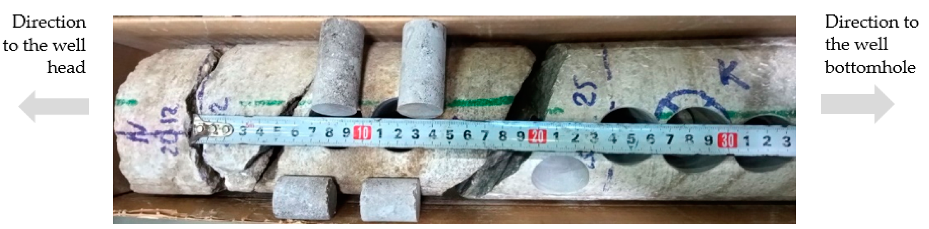
2. Preparation and Description of Carbonate Reservoir Rock Samples

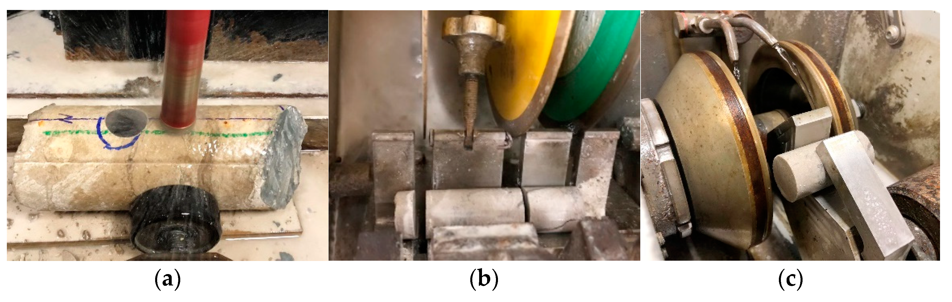
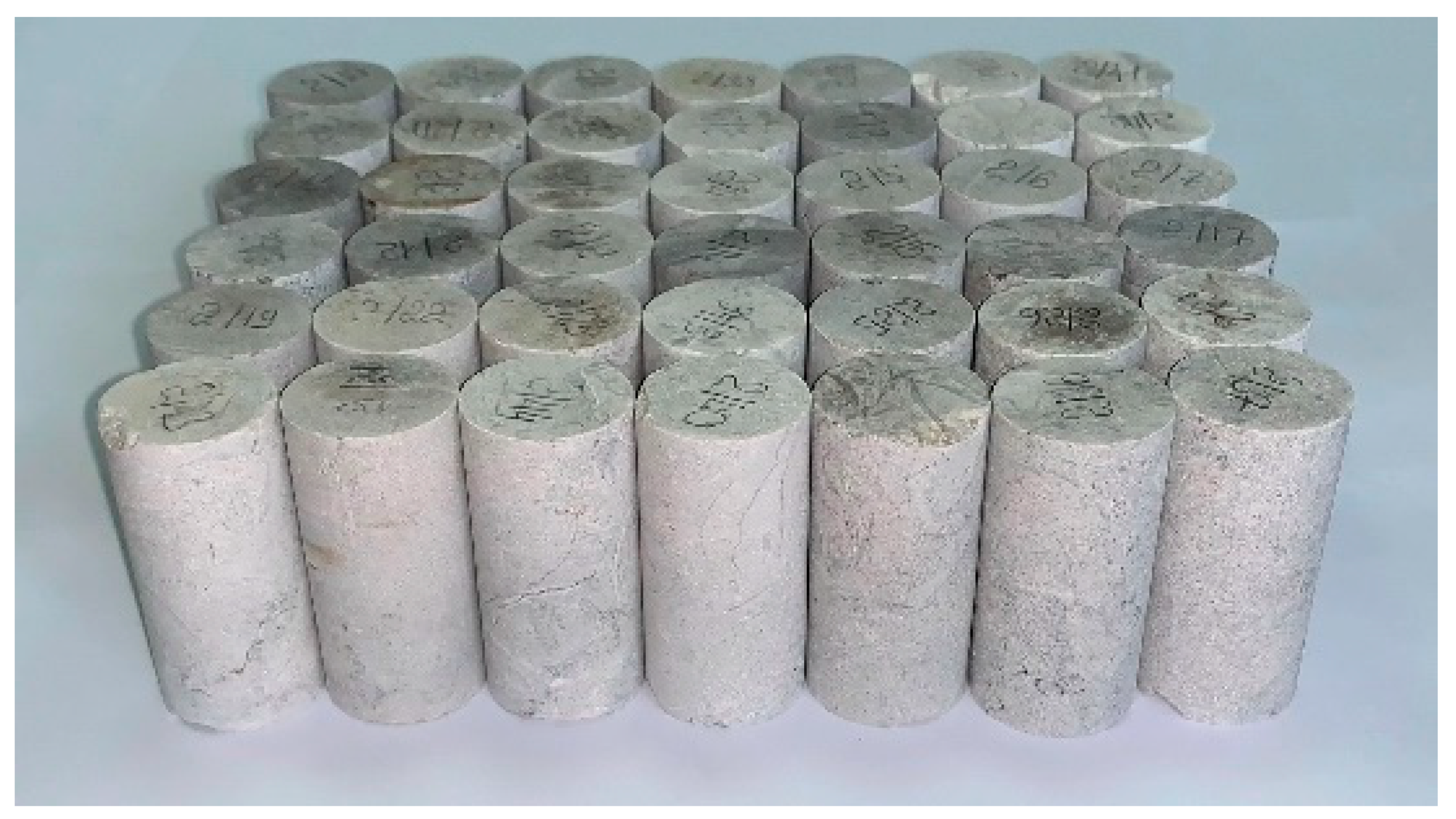
2.1. Preparation of Samples

Carbonate rocks are one of the most common oil-bearing reservoir rocks in the Perm region, Russia. Limestone from one of the oil reservoirs located in the north of the Perm region was selected for the study. The rock is confined to the Bashkir (C₂b) stage of the Middle Carboniferous deposits.

The source material for the preparation of the samples was a core with a diameter of 100 mm, extracted from a depth of 2012–2027 m to the surface while drilling one of the oil producing wells at the oil field. There were three common stages to prepare rock samples for mechanical studies such as drilling, cutting and grinding. At the first stage, rock samples were drilled from the core parallel to the bedding of rocks in such a way that the axis of the samples was perpendicular to the axis of the well (Figure 1). Drilling was performed on the machine using diamond bits with a diameter of d = 25.4 mm, while the core was fixed on the machine using a pusher (Figure 2a). Flushing was performed at all stages of sample preparation for cooling the rock and removing cuttings.

At the second stage, the drilled samples were cut on a disk machine (Figure 2b). The length of the samples was chosen according to the ASTM-4543 standard [32] for mechanical tests as a twice the diameter of the sample l = 50.8 mm. After cutting, the end surfaces of the specimens were ground so that they were parallel to each other (Figure 2c). After manufacturing, the samples were measured and either accepted or rejected if their geometric characteristics did not meet the requirements of the standard.

After preparation, the samples were processed on a Soxhlet apparatus (extractor), on which, according to the standard of the American Petroleum Institute (see Section 4.3 [33]), using an alcohol-benzene mixture, the hydrocarbons contained in the rock were removed within 120 h by hot continuous extraction (Figure 3). One of the possible reasons for the long-term extraction could be the relatively low filtration-capacity properties of the rock. The porosity and permeability measured on the UltraPoroPerm-500 apparatus were 2% and 0.015 μm², respectively.

After extraction, the samples were dried in an oven according to the American Petroleum Institute standard (see Section 3.7 “Drying” [33]) at a temperature of 116 °C until their weight became constant. As a result, 42 samples were prepared for quasi-static and dynamic tests (Figure 4).

2.2. Macroscopic Description

The Limestone samples are detrital and has a light gray color. The structure is fine to micro-grained with a grain size of less than 0.2 mm, different detrital with skeletal forms up to 20 mm in size. The texture is massive. The sample is dense. The bulk is composed of calcite, against the background of which fragments of skeletal forms are observed (fragments of brachiopod shells and scraps of bryozoans are visually accurately diagnosed) up to 20 mm in size. All skeletal forms are malted with calcite. The composition of limestone includes (wt%): calcium Ca (93.62%), silicon Si (3.63%), aluminum Al (1.11%), magnesium Mg (0.88%) and other components. Over the area of the entire sample, finely toothed, branching stylolite seams are observed, filled with a brown clay.

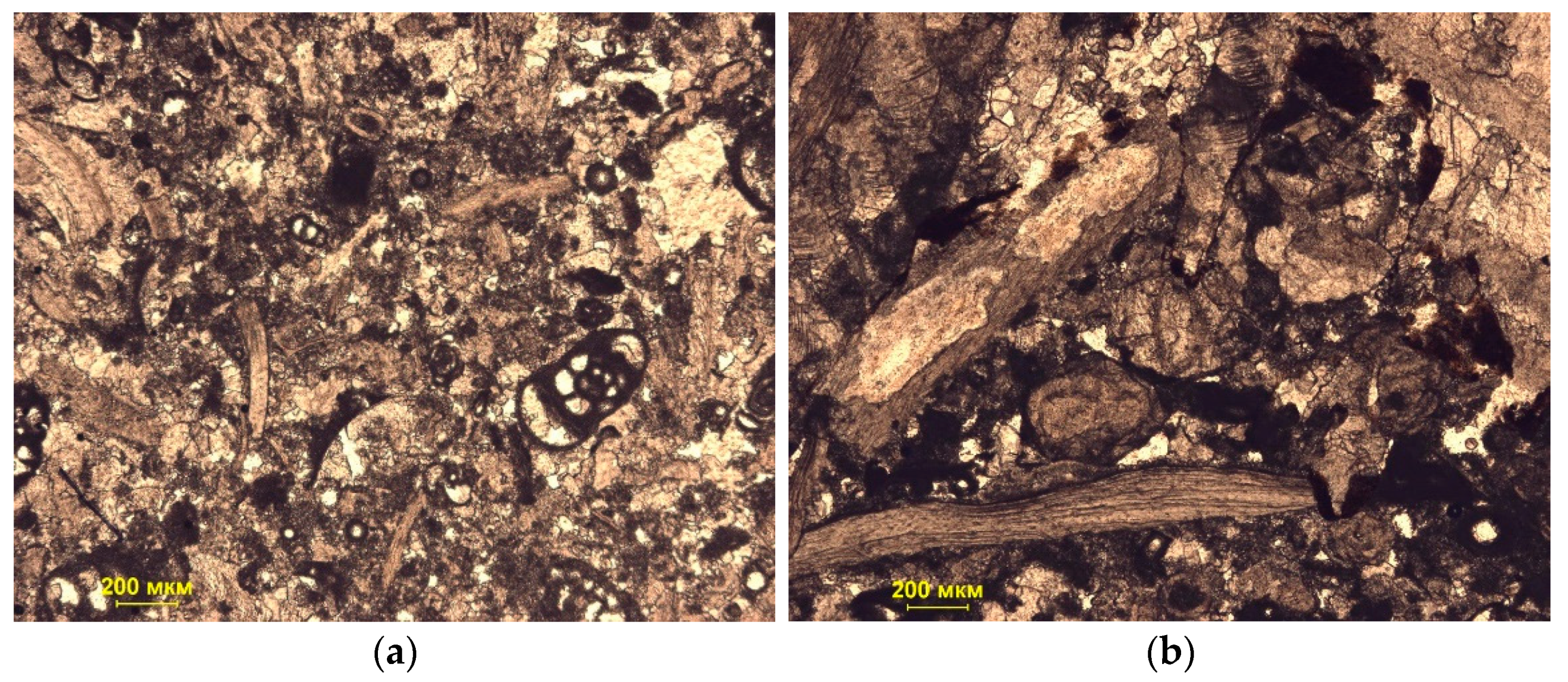
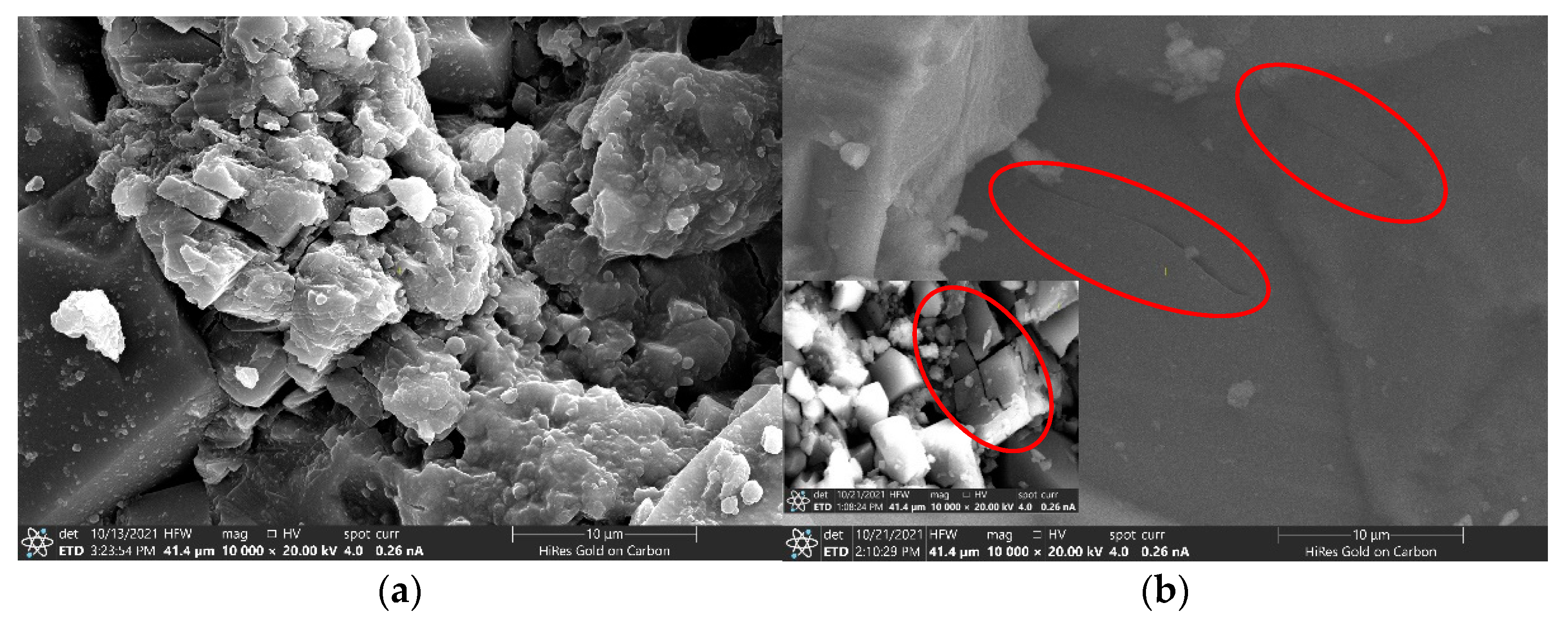
2.3. Microscopic Description

Samples are various-grained bioclastic with micritic matrix with different-crystalline sparite cement. The structure is uneven-grained, pelitomorphic (micritic matrix) to micro-, fine-grained, uneven-detrital. The texture is disordered; no orientation in the arrangement of the constituent parts of the rock is observed in the thin section. Mineral composition: calcite from pelitomorphic (matrix, some shaped components) to different crystalline with a grain size of 0.08–0.3 mm, in the form of xenomorphic and hypidiomorphic crystals (sparite cement, recrystallized shaped components). Shaped components are represented by bioclasts. Bioclasts (~55%): fragments of brachiopod shells 0.18–0.8 mm in size, fragments of ostracod shells 0.1–0.3 mm in size, fragments of foraminifera shells 0.1–0.6 mm in size, a single fragment bryozoans 15 mm in size. The shaped components are composed of micritic calcite, but more often clear crystalline calcite 0.08–0.22 mm in size fills the chambers of bioclasts or fills their walls. Single chambers of skeletal forms are filled with quartz, the grain size of which is less than 0.04 mm. The matrix in the rock is micritic, dark brown, uneven, accounting for ~15% of the thin section area. Secondary calcite cement is sparite (30%), different crystalline with a grain size of 0.08–0.3 mm, developed in the intergranular space as a result of recrystallization of the matrix and bioclasts. Intercrystalline pores, formed along organogenic voids, isolated, rounded, slit-like, irregular in shape. The pores are 0.008–0.2 mm in size. Finely toothed stylolite seams and compaction veins, branching, made with brown clay-organic matter. Micrographs are shown in Figure 5a,b.

The study of limestone under a scanning electron microscope showed that the structure of the sample is represented by a microgranular framework with a rhombohedral calcite particle size of more than 0.1 mm. Some areas of the rock are probably zones of limestone recrystallization with the presence of well-formed densely packed calcite crystals. The cementing agent is represented by aggregates of calcite grains of various shapes less than 10 microns in size and solid precipitates of carbonate matter.

The pore space in the rock is represented, first of all, by micro-caverns with a diameter of up to 0.5 mm, filled with newly formed crystals of calcite. Another part of micropores is represented by intergranular pores up to 0.05 mm in size between relatively larger calcite crystals.

3. Quasi-Static Loading

Quasi-static loading tests were performed to determine the zone of linear elasticity and the main mechanical characteristics of the rock. The tests were carried out at the Center for Experimental Mechanics of the Perm National Research Polytechnic University on a universal electromechanical loading system Instron 5882 using a high-precision independent load cell of the Drop-through type, a Vic-3D systems and an AMSY-6 acoustic emission system. The Vic-3D is a non-contact strain measurement system based on digital image correlation.

The crosshead speed of the loading system under quasi-static loading of rock samples was 2 mm/min. The studies were carried out in accordance with the ASTM standard [34].

While loading the radial strain of rock samples was measured using a mechanical extensometer mounted at the sample perpendicular to the sample’s vertical axis. In order to double check the values of radial strain it was decided to additionally implement a Vic-3D system that uses a speckle structure to register the displacement of regions of the painted picture. Besides, in order to register an internal rock structure deformation (cracking) during quasi-static loading the testing was accomplished with acoustic emission system. Both parts of the quasi-static loading such as measurements of the strain and acoustic emission are discussed below separately in Section 3.1 and Section 3.2 respectively.

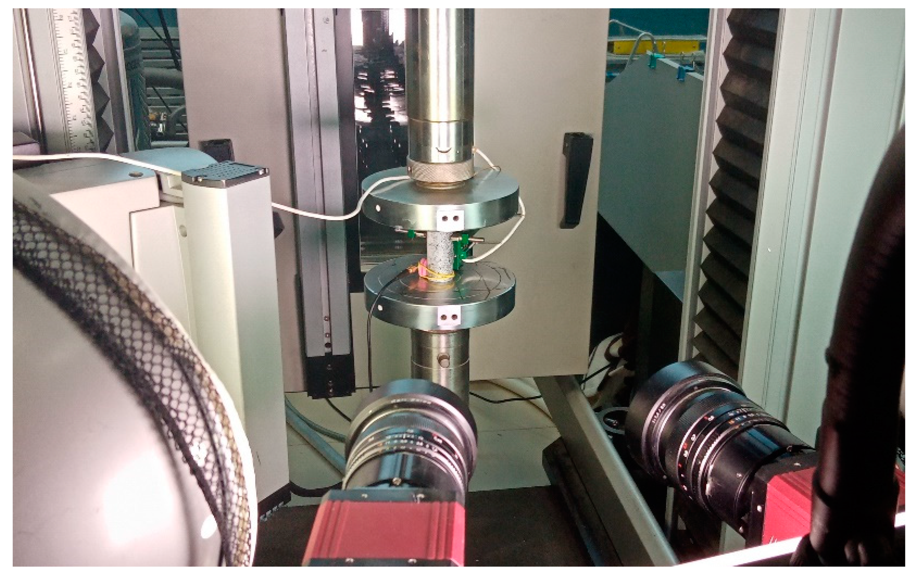
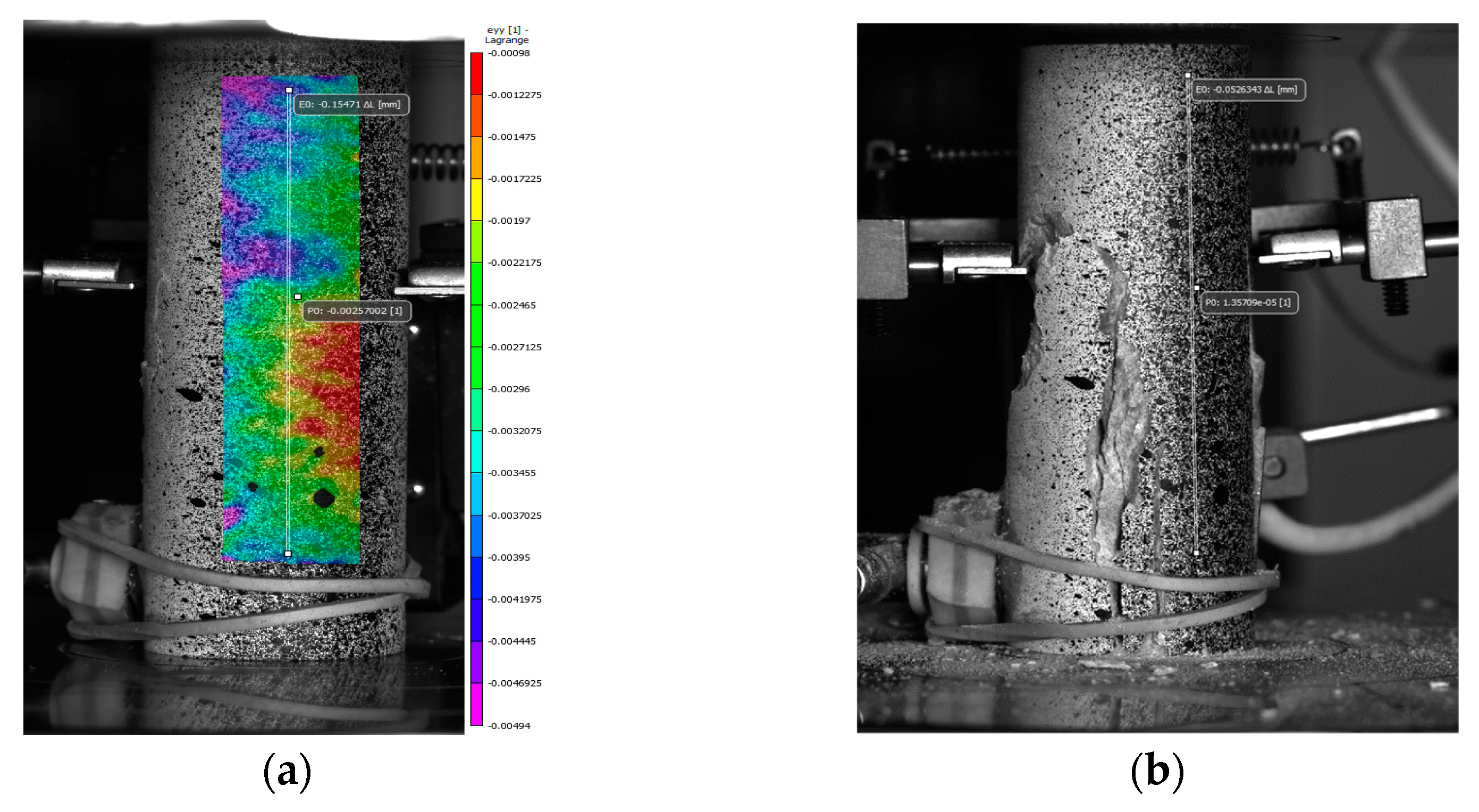
3.1. Measurements of Transversal Deformations with a Mechanical Extensometer and a Vic-3D System

When determining such a mechanical characteristic as Young’s modulus during loading, it is required to measure the longitudinal and transverse deformation. If the longitudinal deformation can be determined on the load stand itself, then the measurement of the transversal deformation requires the use of additional measuring instruments. For that purpose, two systems were used such as Epsilon 3575-250M-ST contact mechanical extensometer and a Vic-3D system. Due to its simplicity, the use of contact mechanical extensometers for testing rocks is widely known and has found application in many experimental works (for example, [35]). Non-contact measuring systems, such as Vic-3D, are also widely used in mechanical testing of rocks (see, for example, [36,37]). The system operates on the Vic-3D digital image correlation technique (Figure 6). Using stamps, the sample is painted, after which a speckle structure (pattern) is formed on the one side of a specimen, which is then registered using two video cameras. During loading, the video cameras record displacement of the areas of a pattern with a resolution of 20 μm/mm while the analysis speed is 85,000 points per second.

The sample deformation process indicators were registered in the Bluehill2 software package, in which the subsequent data processing was carried out. Figure 7a shows an example of loading the sample 14. It can be seen that, during loading, the fracture proceeded along one of the common paths (multiple shear).

As a result of uniaxial compressive strength tests, on stress-strain diagrams the zones of linear elasticity of rock samples were determined. Figure 8 shows an example of the loading diagram for the sample 14. The diagram shows that firstly the sample undergoes elastic deformations (zone of linear elasticity), in which stress and strain are related through Young’s modulus, and then irreversible (plastic) deformations are observed, followed by fracture of the sample. The rock under study was quite tough, the strength of the sample was 137 MPa, and the quasi-static Young’s modulus E_st was equal to 50 GPa. Poisson ration μ was equal to 0.25. The average value of the uniaxial compressive strength ${\sigma }_{UCS}$ for all studied dry and saturated with distilled water samples was equal to 127.6 MPa and 68.8 MPa respectively.

In the experimental work [38] the authors showed that shape deviation of limestone specimens (prepared roughly with no grinding) affects its uniaxial compressive strength and, in particular, that the flatness of the specimen ends is the parameter of the biggest influence on the uniaxial compressive strength. Since the purpose of the quasi-static loading part of the present study was to determine the average limits of the zone of linear elasticity and then go to the main part of dynamic loading, studying the influence of specimen shape deviation was beyond the scope of the present work. However, during preparation of the specimen in the present work the tolerances of ASTM-4543 standard (such as straightness, end flatness, perpendicularity of the ends to the specimen axis and parallelism of the ends) were considered. As a result, there were no influence of shape deviation on the uniaxial compressive strength observed during quasi-static loading.

During quasi-static loading of limestone samples, the fractures propagated in accordance with common failure modes, shown in the Figure 9. For all of the samples there were similar diagram obtained as given in Figure 8. As a result, the zone of linear elasticity was determined. In order to see a moment at a loading diagram where a cracking starts to manifest an acoustic emission (AE) system (described in the following Section 3.2) accomplished the quasi-static loading.

3.2. Acoustic Emission Study

In the process of mechanical testing of the samples, continuous control was carried out by the method of AE. The AE is widely used in the study of the mechanical characteristics of rocks (see, for example, [39]). The AE is a physical phenomenon associated with the emission of elastic waves when a material is loaded and cracks develop. It is based on registration and analysis of waves arising in the process of deformation. For research purposes, broadband piezoelectric acoustic emission transducers (AET) were used with a frequency range of 100–500 kHz (AET-1) and 450-1150 (AET-2) and preamplifiers with a gain of 34 dB. The sensors were attached using a high-vacuum silicone grease to the lateral surface of the sample, as shown in Figure 10.

For the analysis of AE, diagrams of dependences of the main parameters of signals on time were built, which are presented in Figure 11. The AE parameters used in the visualization of the obtained experimental data are the energy parameter (eu) and the number of AE signals. Summing up the values of the energy parameter for all previous time intervals, we can introduce the concept of cumulative energy (E_cum), which reflects the degree of accumulated deformation in the material: $E_{cum}={\displaystyle \sum }_i^n{E}_i$, where $E_i$ is an energy parameter of i-signal of AE.

Figure 11a,b show diagrams of the distribution of the energy parameter of AE signals versus time, combined with the load graph for the entire test period for dry 2/3 and saturated 2/18 samples.

It is seen from Figure 11 that the active growth of the energy parameter begins at the moment preceding the sample fracture. At the initial stage, signals with low values of the energy parameter are recorded. For a dry sample 2/3 (Figure 11a), the energy parameter values are two orders of magnitude less than for sample 2/18 (Figure 11b) saturated with distilled water. It is also seen that the load P for uniaxial compression for a saturated sample is half the load for a dry sample. Figure 11c,d show diagrams of the distribution of the number of registered AE signals versus time, combined with the loading graph for samples 2/3 and 2/18 respectively. It is noted that for both samples an active increase in the number of registered AE signals is observed at the time moment preceding the destruction of the sample and correlates with the distribution of the energy parameter in Figure 11a,b. The total number of registered signals for sample 2/3 was 696 units for sample 2/18 was 623 units.

The results of the study by the AE method showed that in the range of loads from up to 40 kN, no fracture is observed in dry samples and their structure is preserved. This fact is one of the limitations (conditions) when choosing the load amplitude during subsequent studies on dynamic loading of samples. Taking into account the data on quasi-static loading for all tested samples, it was decided that in experiments on nonlinear loading, the dynamic load $F_{dyn}$ should not exceed 10 kN.

4. Dynamic Loading

Using the results of the quasi-static loading, and the limit of the linear elasticity zone in particular, dynamic tests were performed. During the nonlinear dynamic loading test the samples first were statically preloaded with $F_{st}$ in order to allow the rock to get compacted and ensuring that the rock gets the linear elastic deformations and then the samples went through vibration impact (the samples were loaded in different dynamic regimes). The dynamic tests consisted of load-unload cycles. During the nonlinear loading hysteresis loops were observed. In Section 4.1 and Section 4.2 the methodology for the dynamic tests is escribed.

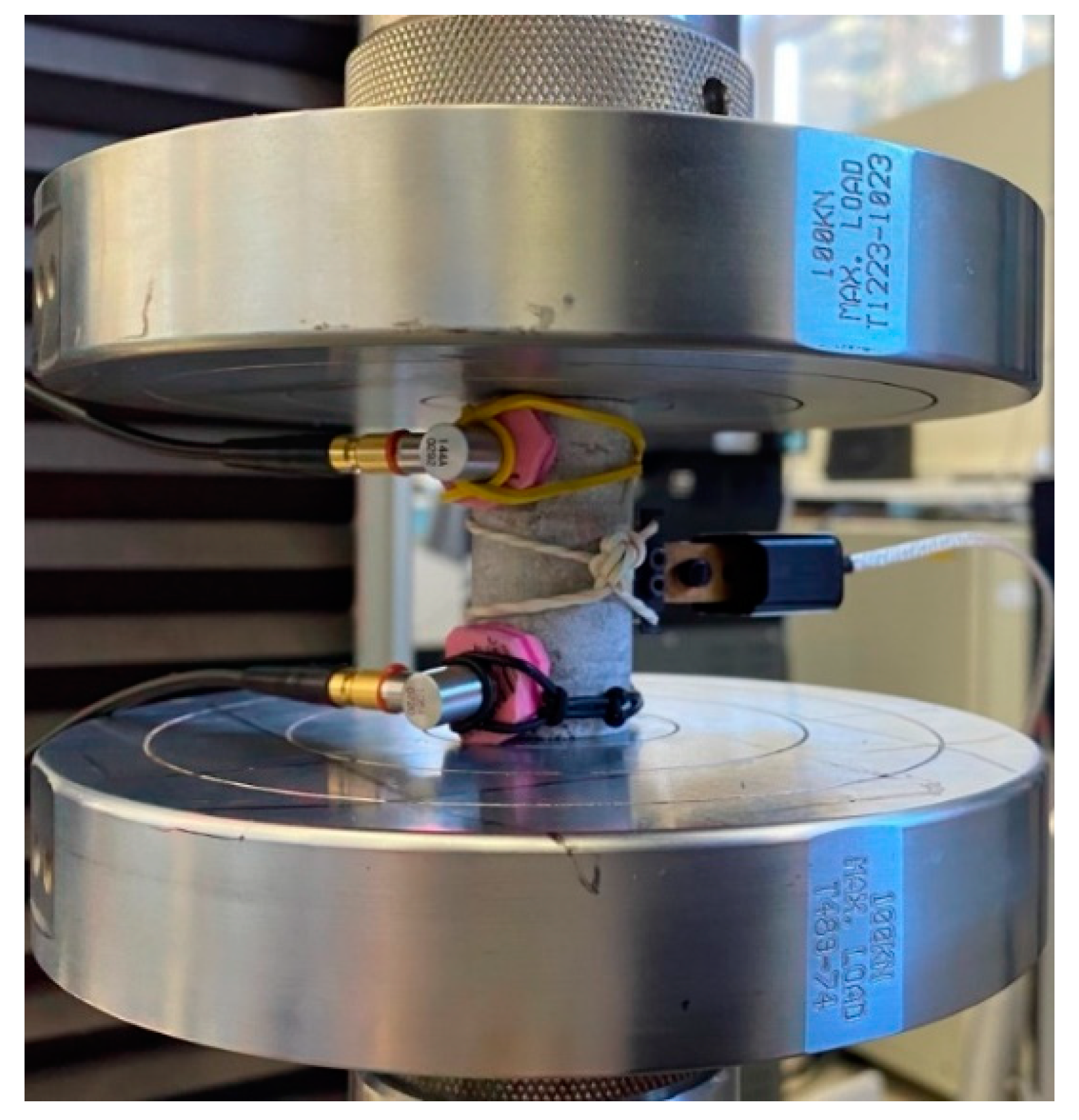
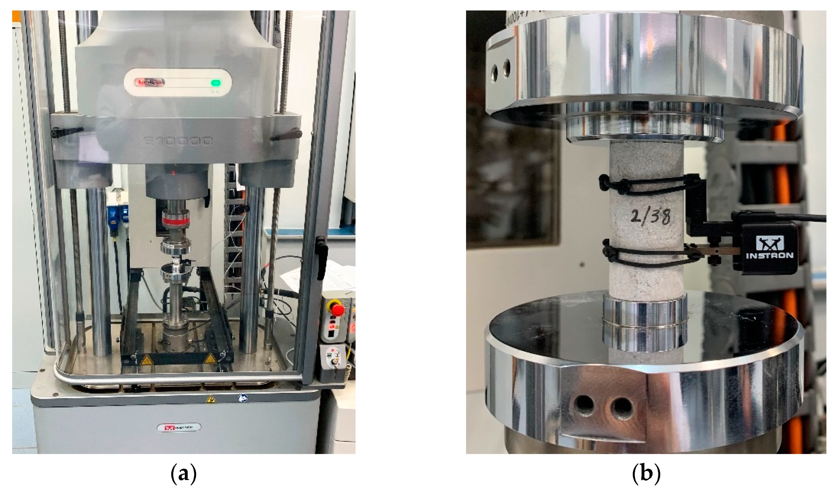
4.1. Description of the Dynamic Experiment

Dynamic tests were carried out at a load corresponding to the initial section of the zone of linear elasticity (in the stress-strain diagram) of the rock, which was determined during quasi-static tests (see Figure 9). Loading was performed on an Instron ElectroPuls E10000 test system. The ElectroPuls system allows to control the actuator with high precision by force (control channel: “load”), by position (control channel “digital displacement sensor”). The “digital displacement sensor” channel has the best frequency characteristics.

The ElectroPuls dynamic testing system has the ability to set acceleration limits and sample break detection settings to allow the system to return to a stable state. Work limits also allow to set thresholds for maximum and minimum forces, displacements, and deformations. A general view of the test system with an installed sample 2/38 and an Instron 2620-603 mechanical dynamic strain gauge (velocity range from 0 to 100 Hz) is shown in Figure 12.

Before dynamic testing the dynamic strain gauge was calibrated on the Epsilon 3590AT calibration stand. The sensor was mounted on knives on the sample side (the distance between the knives was 2.5 cm), located along the edges of the gauge and fixed using rubber cuffs. Before carrying out the experiments, the sensor readings were reset to zero. During the tests, the sensor recorded the longitudinal deformation of the sample caused by the dynamic load with the amplitude $F_a$, changing with the frequency f. The tests were carried out at three amplitudes. The loading amplitude was monitored using the channel of a digital displacement transducer. The amplitude was determined as the ratio of the specified displacement of the actuator to the height of the sample and was selected from the values of 0.01%, 0.02% and 0.03%.

Before dynamic testing the dynamic strain gauge was calibrated on the Epsilon 3590AT calibration stand. The sensor was mounted on knives on the sample side (the distance between the knives was 2.5 cm), located along the edges of the gauge and fixed using rubber cuffs.

Before carrying out the experiments, the sensor readings were reset to zero. During the tests, the sensor recorded the longitudinal deformation of the sample caused by the dynamic load with the amplitude $F_a$, changing with the frequency f. The tests were carried out at three amplitudes. The loading amplitude was monitored using the channel of a digital displacement transducer. The amplitude was determined as the ratio of the specified displacement of the actuator to the height of the sample and was selected from the values of 0.01%, 0.02% and 0.03%.

4.2. Description of the Dynamic Loading Technique

Before the start of the test, the sample was preloaded with a load $F_{st}$ = 6.9 kN, which ensured the closure of microstructures in the rock and transferred the sample to a state of linear elasticity. Then, dynamic loading was carried out with a load amplitude $F_a$ = 850 N. The dynamic loading test program included 9 modes. In each mode, a rock sample was loaded with frequencies $f$ from 0.1 to 60 Hz. The modes were implemented sequentially. The duration of the modes was determined by the number of cycles. The number of cycles for each mode was determined experimentally from the condition of stabilization of the value of the measured parameter (

Table 1. Dynamic loading program.

Loading frequency f, Hz	0.1	0.5	1	2	5	10	20	40	60
Number of cycles N	10	25	50	50	100	200	500	1000	1000

). After the end of each mode, the load on the sample was instantly removed (the sample seemed to relax) and the next mode was immediately implemented, in which the load again reached the specified value.

At each loading mode in the last cycles (where the data were stable), the sample deformation was recorded using a mechanical extensometer, and the load was recorded using a load stand sensor. Data were recorded with a frequency 10⁻³. Figure 13 shows a fragment of the recorded experimental data (cycles 80–82) under dynamic loading of a dry sample 2/46 at a frequency f = 1 Hz. It can be seen from the figure that the maximum amplitude of the dynamic load $F_a$ (Figure 13a) corresponds to the maximum values of the amplitude of the longitudinal deformation ${\epsilon }_a$ of the sample (Figure 13b) and the amplitude of the stress ${\sigma }_a$ in the sample (Figure 13c).

Then, the data was processed in the WaveMatrix package with an additional DMA module. As an example, Figure 14 shows the experimental data obtained under dynamic loading of a dry sample 2/46. It can be seen from the figure that for each frequency of the dynamic load, the values of the strain amplitude and the load amplitude become constant with the number of cycles. At the same time, with an increase in the frequency of the dynamic load, which does not change from one frequency to another one (Figure 14b), the amplitude of the change in longitudinal strain ${\epsilon }_a$ decreases from 0.0029 to 0.0023% (Figure 14a). One of the possible reasons for this phenomenon is that under the higher strain rates the rock gets stiffer in comparison with rock subjected to smaller strain rate dynamic loading.

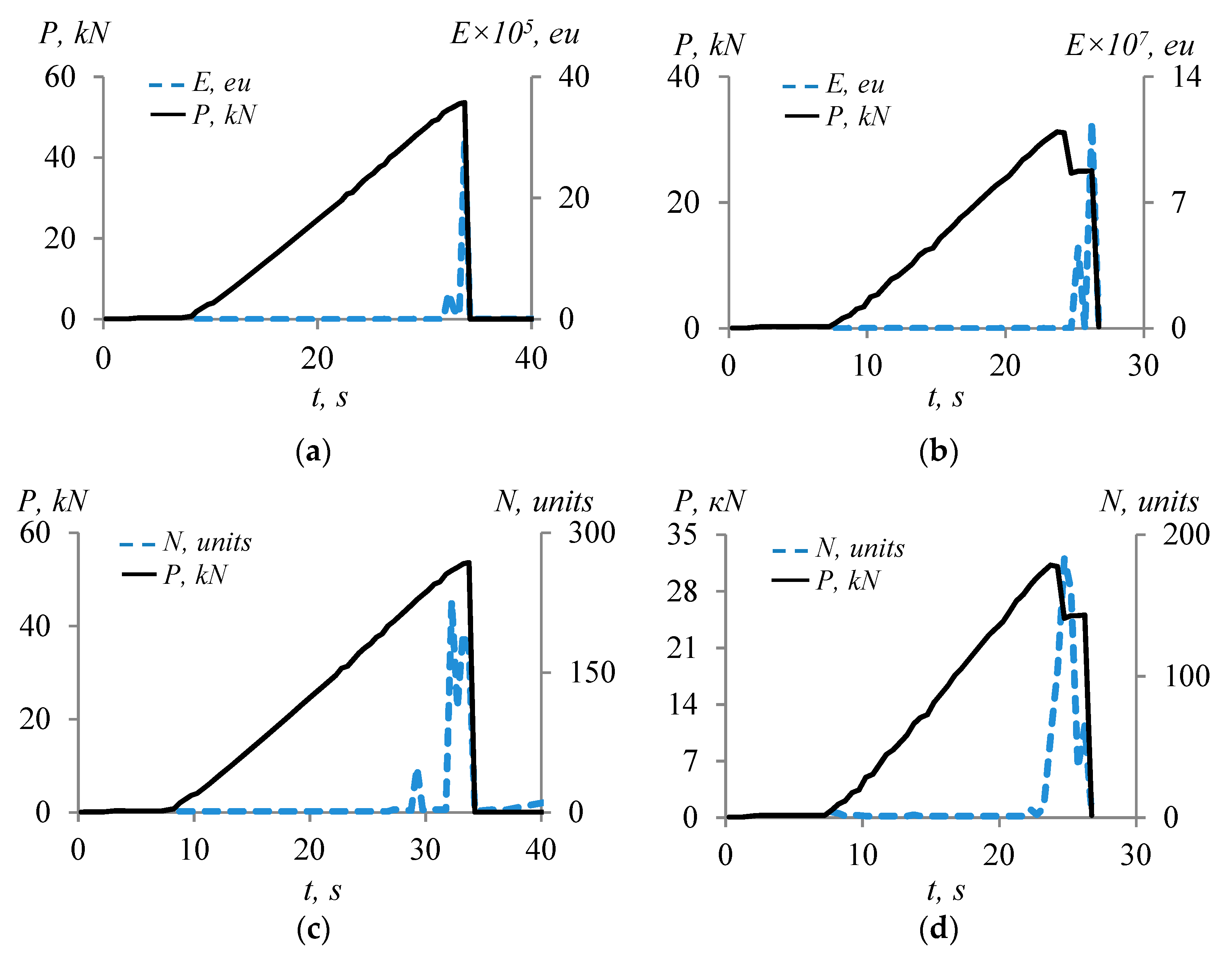
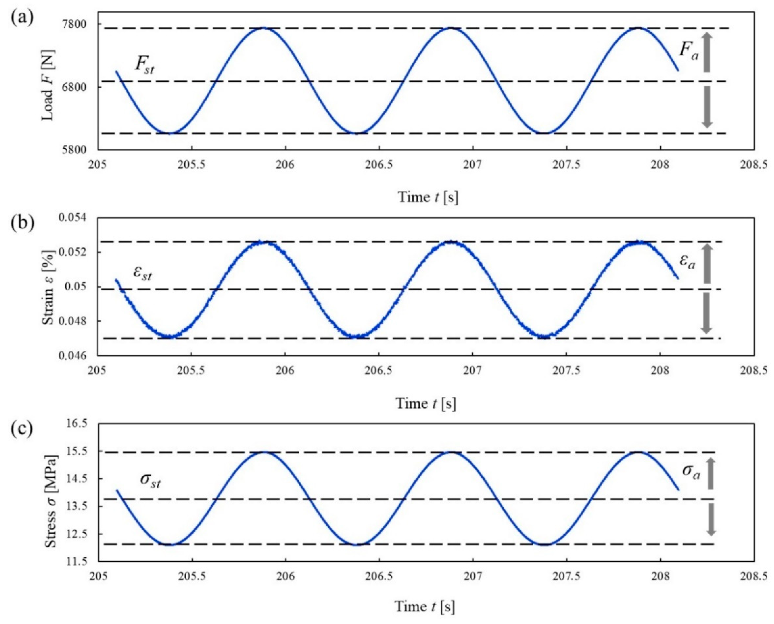
4.3. Data Processing

Dynamic experimental studies of rocks are widely used to study the dynamic mechanical characteristics, usually revealing their dependencies on the load rate. One of the experimental methods for determining the dynamic mechanical characteristics of a material is dynamic mechanical analysis (DMA) using an electrodynamic testing machine and specialized software. On the stress-strain diagram, the loop area as well as the shear angle between stress and strain characterize the amount of dissipated mechanical energy in the rock sample.

Data processing was carried out using the mathematical apparatus of the DMA module. Dynamic modulus of elasticity $E^{*}$ is calculated by the formula $E^{*}=\frac{\Delta \sigma }{\Delta \epsilon }=E^{\prime }+i{E}^{″}=\sqrt{{\left(E^{\prime }\right)}^2+{\left(E^{″}\right)}^2}$, in which $E^{\prime }$ is the real part of the complex modulus of elasticity, defined as $E^{\prime }=E^{*}\times \cos {\phi }_E$, and $E^{″}$ is the imaginary part of the complex elastic modulus defined as $E^{″}=E^{*}\times \sin {\phi }_E$. The phase shift angle ${\phi }_E$ (deg.) between stress and strain (loss angle) is determined by the formula ${\phi }_E=arc\sin \left(\frac{a}{\pi \times \frac{\Delta u}{2}\times \frac{\Delta F}{2}}\right)=arc\tan \left(\frac{E^{″}}{E^{\prime }}\right)$, wherein $\Delta u$ is dedicated to peak-to-peak displacement (mm), $\Delta F$ is a peak-to-peak force (N), $a$ is an energy (J) or area limited by a hysteresis loop (integral of force over displacement) $a={{\displaystyle \oint }}_{u_{min}}^{u_{max}}Fdu$.

5. Results of Dynamic Loading

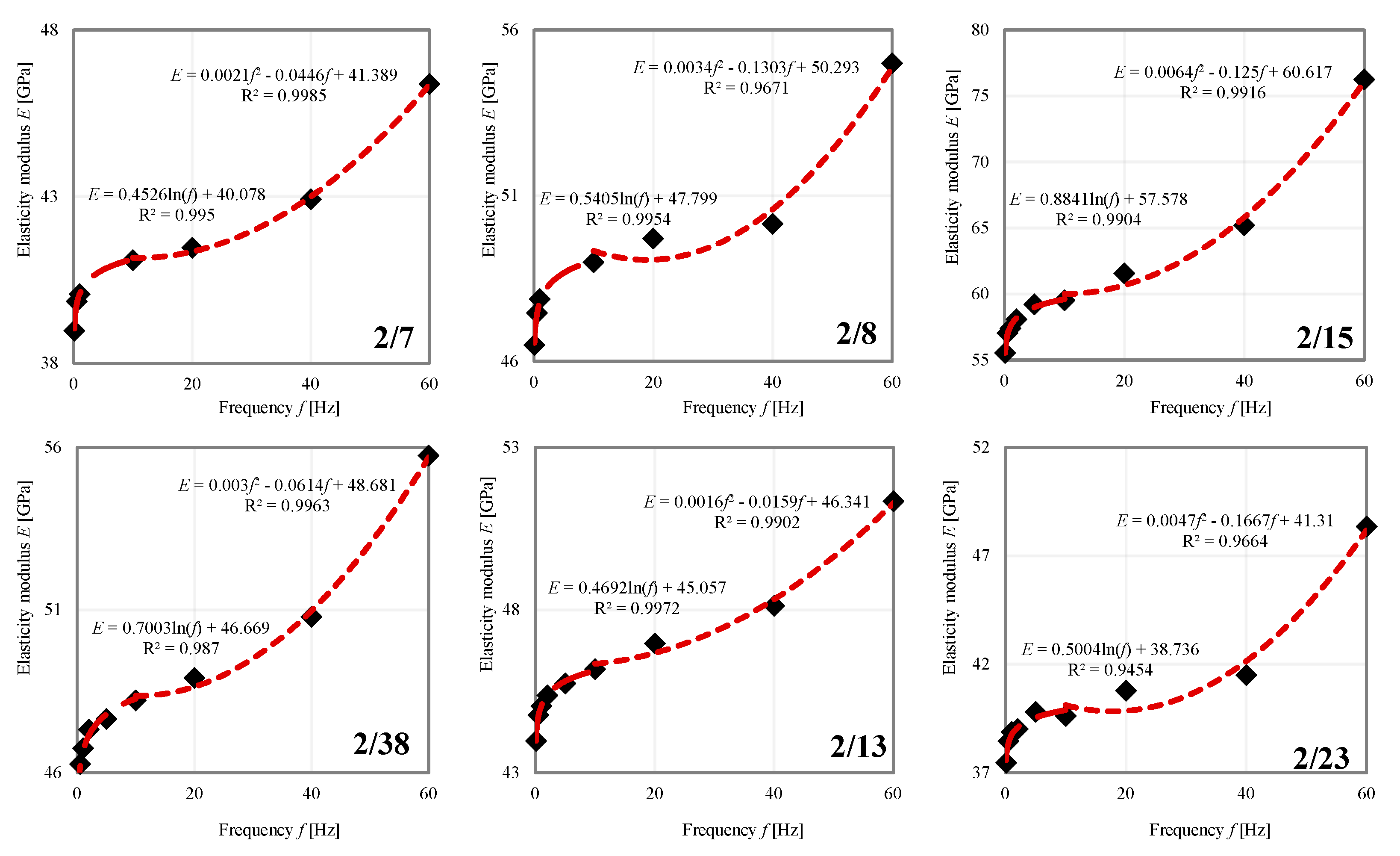
5.1. Dependence of an Elasticity Modulus on the Dynamic Load Frequency

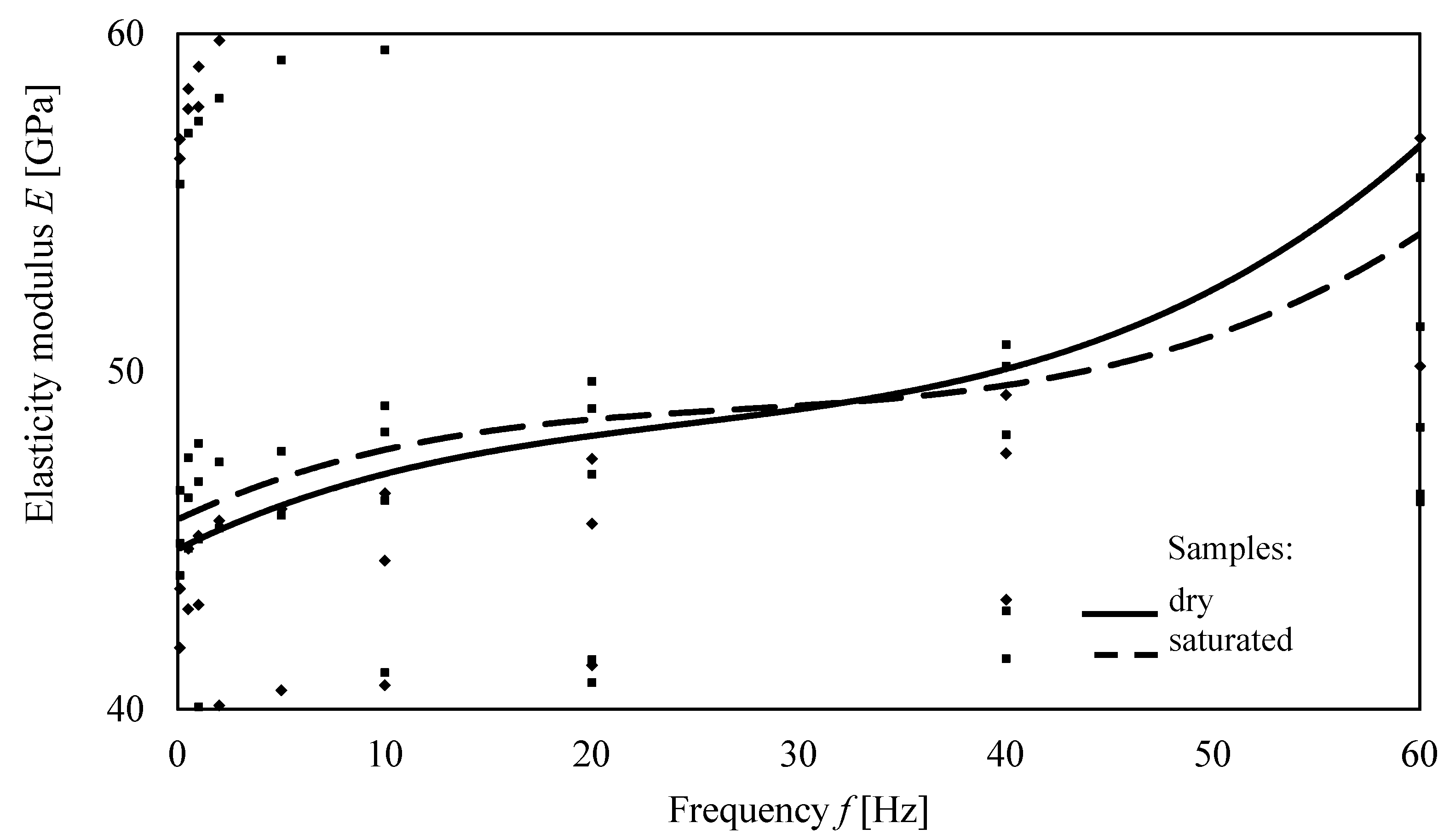
Nonstationary loading of the samples revealed nonlinearity in the behavior of the dynamic modulus of elasticity. Moreover, if in the region of higher frequencies (from 10 Hz to 60 Hz) the test results confirmed the previously obtained dispersion of Young’s modulus according to the power law (see, for example, [24,25,26,27,28]), then in the region of low frequencies (less than 10 Hz) it was revealed that Young’s modulus changes according to the kind of logarithmic law. Figure 15 shows an example of a dynamic test for the sample 2/6. In the absence of a dynamic load, Young’s modulus tends to the value under quasi-static loading (58.2 GPa). It can be seen that in the frequency range f from 10 to 20 Hz, the logarithmic law of Young’s modulus changes is replaced by a quadratic one.

It can be said that the vacuum saturation of the samples with distilled water does not significantly affect the nature of the dependences—the behavior of Young’s modulus is also described with high accuracy by the logarithmic and power laws (Figure 16). At the same time, when averaging the experimental data, it can be seen that the characteristic curve of Young’s modulus behavior for saturated samples has a smoother shape in comparison with the curve for dry samples (Figure 17). The weights of the tested dry and saturated samples were 66 g and 67 g, respectively.

In all loading modes of dry sample 2/46, as in loading other samples (including saturated ones), a hysteresis loop was observed (Figure 18a), which was also revealed, for example, in [40]. For the tested samples a phase angle ${\phi }_E$ was in the range from 0.4 to 4.8 deg. It is noted that up to a load frequency f of 20 Hz, the dependence of the phase angle ${\phi }_E$ from frequency is absent. At the same time, after a frequency of 20 Hz, the phase angle (and, accordingly, the dissipated energy) decreases (Figure 18b).

5.2. Discussion

According to the results of dynamic experiments, an excess of the dynamic modulus of elasticity over the static one is observed. There is an opinion that the excess of the dynamic Young’s modulus over the static one is directly related to the deformation rate and the loading method [16]. The change in the dynamic elastic characteristics of rocks at high deformations is described by existing models, for example, using the inertial approach [13]. However, the mechanism by which the dispersion of the dynamic component of Young’s modulus occurs remains not fully disclosed. To study the nonlinear nature of the dynamic component of the modulus of longitudinal elasticity under the influence of dynamic loads, the authors carried out experimental studies of dry sandstone New Red in the zone of linear elasticity under uniaxial compression and proposed physically substantiated relationships.

The experimental results (see Figure 15 and Figure 16) indicate the presence of two laws, in accordance with which there is a change in the modulus of elasticity when the frequency of the applied load changes. In the existing theoretical and experimental works, there are not many dependencies that describe the change in the elastic modulus of a rock under the action of a dynamic load. In [41] a classical model (based on the model of Jaeger J.C. [42]) is presented for clastic rock, which is capable of describing the behavior (dispersion) of the dynamic modulus of elasticity in accordance with a power law on the basis of physically substantiated relations. Gradient models (see for example [43,44]) can be considered as a non-classical model capable of reflecting the variance of Young’s modulus. Gradient models allow to take into account the heterogeneity of the material structure when describing the change in its elastic characteristics. The additive in the model is responsible for the dispersion of the dynamic Young’s modulus observed under unsteady loading of a rock sample. The indicated classical and non-classical models will be valid for the frequency range corresponding to the quadratic dispersion of the elastic modulus (that is, according to the results obtained in this work, from 10 to 60 Hz). In the case of the low frequency region, it is required to compile models that take into account logarithmic or fractional rational functions.

Experimental data diagrams of dynamic elastic modulus in logarithmic coordinates are shown in Figure 19.

As a result of comparison of electron microscopy of the sample with a magnification of 10⁴ before dynamic loading tests (Figure 20a) and after dynamic loading, it was revealed that the microcracks were formed in the limestone structure. Despite the fact that the loading of the samples was carried out in the zone of linear elasticity in the photographs, fractured calcium crystals are observed, that was not observed before the dynamic loading (Figure 20b).

6. Conclusions

The research program on prepared specimens was conducted to examine what is the influence of nonlinear dynamic loads on such the mechanical characteristic as the dynamic Young’s modulus of carbonate reservoir rocks. Before the tests, rock specimens were drilled, cut and grinded in accordance with corresponding standards. The length of the specimen was 50.8 mm and a diameter was 25.4 mm. After that, in order to determine basic mechanical properties such as the uniaxial compressive strength, Poisson’s ratio, Young’s modulus, and the zone of linear elasticity prepared samples were tested in quasi-static regime. Several measuring systems such as mechanical extensometer and Vic-3D were utilized for quasi-static tests. Just before dynamic loading the sample was statically preloaded to ensure all the microstructures are closed. The investigation was carried out at the strain rate of up to 10⁻³ s⁻¹. In comparison with other studies, we performed not a “one-way” dynamic loading, but dynamic loading at frequencies of up to 60 Hz. According to the presented results following conclusion can be drawn:

• The frequency of the dynamic load applied to the top end of the specimen has a significant impact on the dynamic Young’s modulus which is connected to a higher strain rate. The obtained results can be used for better understanding and optimization of bit-rock interaction since it is shown that during dynamic impact loading (bit bounce) the rock hardens.
• A nonlinear nature of the dynamic Young’s modulus of a carbonate rock was revealed at the frequency ranging from 0.1 to 60 Hz. It was found that with an increase in the frequency from 0.1 to 10 Hz and from 10 to 60 Hz dynamic Young’s modulus rises according to a logarithmic and then to power law for each value of loading amplitudes.
• With an increase in the strain rate the amplitude of the strain ${\epsilon }_a$ decreases. One of the possible reasons for this phenomenon is that under the higher strain rates the rock gets stiffer in comparison with rock subjected to smaller strain rate dynamic loading.
• Despite the effect of water on mechanical properties of specimens determined during quasi-static testing, there were no significant change in dynamic Young’s modulus observed during nonlinear dynamic loading.

References

1. Deng, J.; Liu, C.; Liu, J. Effect of dynamic loading on mechanical properties of concrete. Adv. Mat. Res. 2012, 568, 147–153. [Google Scholar] [CrossRef]
2. Redmann, A.; Montoya-Ospina, M.C.; Karl, R.; Rudolph, N.; Osswald, T.A. High-force dynamic mechanical analysis of composite sandwich panels for aerospace structures. Compos. Part C Open Access 2021, 5, 100136. [Google Scholar] [CrossRef]
3. Tang, B.; Ren, Y. Study on Seismic Response and Damping Measures of Surrounding Rock and Secondary Lining of Deep Tunnel. Shock Vib. 2021, 2021, 7824527. [Google Scholar] [CrossRef]
4. Xu, J.; Kang, Y.; Liu, F.; Liu, Y.; Wang, Z.; Wang, X. Mechanical properties and fracture behavior of flawed granite under dynamic loading. Soil Dyn. Earthq. Eng. 2021, 142, 106569. [Google Scholar] [CrossRef]
5. Dong, L.-X.; Wang, S.-H. Research on dynamic characteristic of marine shafting-oil film-stern structure system. J. Dyn. Syst. Meas. Control Trans. ASME 2019, 141, 021001. [Google Scholar] [CrossRef]
6. Zhang, S.; Caprani, C. Mechanical properties of pultruded GFRP at intermediate strain rates. Compos. Struct. 2021, 278, 114699. [Google Scholar] [CrossRef]
7. Nguyen, K.-L.; Tran, Q.-T.; Andrianoely, M.-A.; Manin, L.; Baguet, S.; Dufour, R.; Mahjoub, M.; Menand, S. Nonlinear rotordynamics of a drillstring in curved wells: Models and numerical techniques. Int. J. Mech. Sci. 2020, 166, 105225. [Google Scholar] [CrossRef] [Green Version]
8. Kamel, J.M.; Yigit, A.S. Modeling and analysis of stick-slip and bit bounce in oil well drillstrings equipped with drag bits. J. Sound Vib. 2014, 333, 6885–6899. [Google Scholar] [CrossRef]
9. Yigit, A.S.; Christoforou, A.P. Stick-Slip and Bit-Bounce Interaction in Oil-Well Drillstrings. J. Energy Res. Technol. 2006, 128, 268. [Google Scholar] [CrossRef]
10. Fushen, R.; Baojin, W. Modeling and analysis of stick-slip vibration and bit bounce in drillstrings. J. Vibroengineering 2017, 19, 4866–4881. [Google Scholar] [CrossRef]
11. Wiercigroch, M.; Vaziri, V.; Kapitaniak, M. RED: Revolutionary Drilling Technology for Hard Rock Formations. In Proceedings of the Society of Petroleum Engineers—IADC/SPE Drilling Conference and Exhibition 2017: SPE/IADC Drilling Conference and Exhibition, The Hague, The Netherlands, 14–16 March 2017; Society of Petroleum Engineers (SPE). pp. 1234–1241. [Google Scholar] [CrossRef]
12. Qi, X.; Chen, W.; Liu, Y.; Tang, X.; Shi, S. A Novel Well Drill Assisted with High-Frequency Vibration Using the Bending Mode. Sensors 2018, 18, 1167. [Google Scholar] [CrossRef] [PubMed] [Green Version]
13. Zhang, Q.B.; Zhao, J. A Review of Dynamic Experimental Techniques and Mechanical Behaviour of Rock Materials. Rock Mech. Rock Eng. 2014, 47, 1411–1478. [Google Scholar] [CrossRef] [Green Version]
14. Xu, Y.; Zhang, H.; Guan, Z. Dynamic Characteristics of Downhole Bit Load and Analysis of Conversion Efficiency of Drill String Vibration Energy. Energies 2021, 14, 229. [Google Scholar] [CrossRef]
15. Zheng, J.; Dou, B.; Li, Z.; Wu, T.; Tian, H.; Cui, G. Design and Analysis of a While-Drilling Energy-Harvesting Device Based on Piezoelectric Effect. Energies 2021, 14, 1266. [Google Scholar] [CrossRef]
16. Peng, K.; Zhou, J.; Zou, Q.; Song, X. Effect of loading frequency on the deformation behaviours of sandstones subjected to cyclic loads and its underlying mechanism. Int. J. Fatigue 2020, 131, 105349. [Google Scholar] [CrossRef]
17. Bijay, K.C.; Foroutan, M.; Ghazanfari, E. Analysis and Comparison of Measured Static and Dynamic Moduli of a Dolostone Specimen. Geotech. Spec. Publ. 2019, 2019, 484–493. [Google Scholar] [CrossRef]
18. Zheng, Q.; Liu, E.; Sun, P.; Liu, M.; Yu, D. Dynamic and damage properties of artificial jointed rock samples subjected to cyclic triaxial loading at various frequencies. Int. J. Rock Mech. Min. Sci. 2020, 128. [Google Scholar] [CrossRef]
19. Jafari, M.K.; Pellet, F.; Boulon, M.; Hosseini, K.A. Experimental Study of Mechanical Behaviour of Rock Joints Under Cyclic Loading. Rock Mech. Rock Eng. 2004, 37, 3–23. [Google Scholar] [CrossRef]
20. Van Massenhove, K.; Debruyne, S.; Vandepitte, D. Variability analysis on the structural elastic properties of adhesively joined cylinders. J. Phys. Conf. Ser. 2016, 744. [Google Scholar] [CrossRef]
21. Xia, K.; Yao, W.; Wu, B. Dynamic rock tensile strengths of Laurentian granite: Experimental observation and micromechanical model. J. Rock Mech. Geotech. Eng. 2017, 9, 116–124. [Google Scholar] [CrossRef]
22. Liu, X.; Dai, F.; Liu, Y.; Pei, P.; Yan, Z. Experimental investigation of the dynamic tensile properties of naturally saturated rocks using the coupled static–dynamic flattened brazilian disc method. Energies 2021, 14, 4784. [Google Scholar] [CrossRef]
23. Meng, L.; Han, L.; Meng, Q.; Liu, K.; Tian, M.; Zhu, H. Study on characteristic and energy of argillaceous weakly cemented rock under dynamic loading by Hopkinson bar experiment. Energies 2020, 13, 3215. [Google Scholar] [CrossRef]
24. Pimienta, L.; Fortin, J.; Guéguen, Y. Bulk modulus dispersion and attenuation in sandstones. Geophysics 2015, 80, D111–D127. [Google Scholar] [CrossRef]
25. Lozovyi, S.; Bauer, A. Static and dynamic stiffness measurements with Opalinus Clay. Geophys. Prospect. 2019, 67, 997–1019. [Google Scholar] [CrossRef]
26. Holt, R.M.; Lozovyi, S.; Pohl, M.; Szewczyk, D. Frequency-dependent wave velocities in sediments and sedimentary rocks: Laboratory measurements and evidences. Lead. Edge 2016, 35, 474–560. [Google Scholar] [CrossRef] [Green Version]
27. Borgomano, J.V.M.; Gallagher, A.; Sun, C.; Fortin, J. An apparatus to measure elastic dispersion and attenuation using hydrostatic- and axial-stress oscillations under undrained conditions. Rev. Sci. Instrum. 2020, 91, 034502. [Google Scholar] [CrossRef] [PubMed]
28. Guzev, M.A.; Kozhevnikov, E.V.; Turbakov, M.S.; Riabokon, E.P.; Poplygin, V.V. Experimental studies of the influence of dynamic loading on the elastic properties of sandstone. Energies 2020, 13, 6195. [Google Scholar] [CrossRef]
29. Spencer Jr, J.W. Stress relaxations at low frequencies in fluid-saturated rocks: Attenuation and modulus dispersion. J. Geophys. Res. 1981, 86, 1803–1812. [Google Scholar] [CrossRef]
30. Szewczyk, D.; Bauer, A.; Holt, R.M. A new laboratory apparatus for the measurement of seismic dispersion under deviatoric stress conditions. Geophys. Prospect. 2016, 64, 789–798. [Google Scholar] [CrossRef] [Green Version]
31. Mikhaltsevitch, V.; Lebedev, M.; Gurevich, B. A laboratory study of the elastic and anelastic properties of the sandstone flooded with supercritical CO2 at seismic frequencies. Energy Procedia 2014, 63, 4289–4296. [Google Scholar] [CrossRef] [Green Version]
32. ASTM D4543: Standard Practices for Preparing Rock Core Specimens and Determining Dimen-Sional and Shape Tolerances; American Society for Testing and Materials International: West Conshohocken, PA, USA, 2001.
33. Recommended Practices for Core Analysis. Recommended Practice 40, 2nd ed.; American Petroleum Institute: Washington, DC, USA, 1998. [Google Scholar]
34. ASTM D7012-14e1, Standard Test Methods for Compressive Strength and Elastic Moduli of Intact Rock Core Specimens under Varying States of Stress and Temperatures; ASTM International: West Conshohocken, PA, USA, 2014.
35. Fujii, Y.; Kiyama, T.; Ishijima, Y.; Kodama, J. Examination of a rock failure criterion based on circumferential tensile strain. Pure Appl. Geophys. 1998, 152, 551–577. [Google Scholar] [CrossRef]
36. Zhang, H.; Nath, F.; Parrikar, P.N.; Mokhtari, M. Analyzing the validity of Brazilian testing using digital image correlation and numerical simulation techniques. Energies 2020, 13, 1441. [Google Scholar] [CrossRef] [Green Version]
37. Chen, C.; Xu, J.; Okubo, S.; Peng, S. Damage evolution of tuff under cyclic tension–compression loading based on 3D digital image correlation. Eng. Geol. 2020, 275, 105736. [Google Scholar] [CrossRef]
38. Štambuk Cvitanović, N.; Nikolić, M.; Ibrahimbegović, A. Influence of specimen shape deviations on uniaxial compressive strength of limestone and similar rocks. Int. J. Rock Mech. Min. Sci. 2015, 80, 357–372. [Google Scholar] [CrossRef]
39. Sirdesai, N.N.; Gupta, T.; Singh, T.N.; Ranjith, P.G. Studying the acoustic emission response of an Indian monumental sandstone under varying temperatures and strains. Constr. Build. Mater. 2018, 168, 346–361. [Google Scholar] [CrossRef]
40. Tutuncu, A.N.; Podio, A.L.; Gregory, A.R.; Sharma, M.M. Nonlinear viscoelastic behavior of sedimentary rocks, Part I: Effect of frequency and strain amplitude. Geophysics 1998, 63, 184–194. [Google Scholar] [CrossRef]
41. Guzev, M.; Riabokon, E.; Turbakov, M.; Kozhevnikov, E.; Poplygin, V. Modelling of the dynamic Young’s modulus of a sedimentary rock subjected to nonstationary loading. Energies 2020, 3, 6461. [Google Scholar] [CrossRef]
42. Jaeger, J.C.; Cook, N.G.W.; Zimmerman, R.W. Laboratory testing of rocks. In Fundamentals of Rock Mechanics, 4th ed.; Blackwell Publishing: Malden, MA, USA, 2007; pp. 145–167. [Google Scholar]
43. Qi, C.Z.; Li, K.R.; Bai, J.P.; Chanyshev, A.I.; Liu, P. Strain gradient model of zonal disintegration of rock mass near deep-level tunnels. J. Min. Sci. 2017, 53, 21–33. [Google Scholar] [CrossRef]
44. Lavrikov, S.V.; Revuzhenko, A.F. Mathematical Modeling of Deformation of Self-Stress Rock Mass Surrounding a Tunnel. In Desiderata Geotechnica; Springer: Cham, Switzerland, 2019; pp. 79–85. [Google Scholar] [CrossRef]
Figure 1. Core extracted from the subsurface while drilling an oil producing well at the field located in the north of the Perm region and limestone samples cut with 25.4 mm diameter diamond bits.
Energies 14 08559 g001
Figure 2. Stages of preparation of rock samples: (a) drilling of samples with a diameter of 25.4 mm; (b) cutting samples with a length of 50.8 mm; (c) grinding end surfaces to ensure parallelism.
Energies 14 08559 g002
Figure 3. Extraction of hydrocarbons from prepared carbonate rock samples.
Energies 14 08559 g003
Figure 4. Prepared cylindrical samples of carbonate rock.
Energies 14 08559 g004
Figure 5. Micrographs of a thin section made from a rock sample: (a) fragments of shells of brachiopods, foraminifera, ostracods cemented with secondary calcite sparite cement; (b) a fragment of a brachiopod shell, the chamber of which is made of quartz grains, a fragment of a stylolite suture.
Energies 14 08559 g005
Figure 6. General view of the Vic-3D system at the moment of loading a rock sample on the Instron 5882 setup. Two cameras record the speckle structure displacement.
Energies 14 08559 g006
Figure 7. Images of the rock sample 14 with a speckle structure painted at the one side of the sample taken using the Vic 3D strain field registration system: (a) during the test; (b) after the test.
Energies 14 08559 g007
Figure 8. The diagram showing stress σ versus strain ε dependency during quasi-static loading of the rock sample 11. At the first stage the linear section is observed corresponding to the elastic strain, then plastic deformations are observed until the samples is fractured.
Energies 14 08559 g008
Figure 9. The different modes of failures of rock samples during quasi-static loading: Y-shaped (2/5), double shear (2/10), axial splitting (2/11), shearing along a single plain (2/12, 2/32, 2/45).
Energies 14 08559 g009
Figure 10. The sample with installed AETs and a mechanical extensometer between loading plates.
Energies 14 08559 g010
Figure 11. Diagrams of the dependence of the energy parameter of AE signals on time, combined with the loading curves: (a) dry sample 2/3; (b) saturated sample 2/18; and diagrams of the distribution of the number of registered AE signals versus time, combined with the loading diagram: (c) dry sample 2/3; (d) saturated sample 2/18.
Energies 14 08559 g011
Figure 12. Instron ElectroPuls E10000 Test System with Test Sample: (a) general view of the installation; (b) dry sample 2/38 installed between the loading plates with an Instron 2620-603 dynamic strain gauge.
Energies 14 08559 g012
Figure 13. Experimental data obtained during dynamic loading of a sample 2/46 at a frequency f of 1 Hz (cycles 80–82): (a) dynamic load F with an average F s t and amplitude F a , applied to the sample; (b) longitudinal strain ε of the sample; (c) stress σ in the sample.
Energies 14 08559 g013
Figure 14. Experimental data obtained during the dynamic loading of the sample 2/46 at different loading frequencies f : (a) strain amplitude ε a ; (b) load amplitude F a .
Energies 14 08559 g014
Figure 15. Dynamic modulus of elasticity of dry limestone samples.
Energies 14 08559 g015
Figure 16. Dynamic modulus of elasticity of limestone samples saturated with distilled water.
Energies 14 08559 g016
Figure 17. Dynamic modulus of elasticity of dry and saturated limestone (data averaged over 6 samples shown in Figure 15 and Figure 16) depending on the frequency of the applied dynamic load.
Energies 14 08559 g017
Figure 18. Experimental data obtained during testing the sample 2/46: (a) hysteresis loop at a load frequency of 1 Hz (strain ε is indicated as a percentage); (b) the frequency dependence of the phase angle between stress and strain, as well as the energy dissipated in one cycle of deformation (area of the hysteresis loop) when testing a 2/46 sample at a frequency of 1 Hz.
Energies 14 08559 g018
Figure 19. Diagrams of experimental data for the sample 2/46 versus dynamic load frequency f depending on the strain amplitude εa in logarithmic coordinates: (a) dynamic modulus of elasticity; (b) real part of the modulus of elasticity; (c) imaginary part of the complex elastic modulus; (d) phase shift angle φ E .
Energies 14 08559 g019
Figure 20. Pore space of limestone sample obtained with an electron microscope when analyzing sample 2/46 with magnification of 104: (a) no cracks before the dynamic loading; (b) cracks in calcium crystals after dynamic loading.
Energies 14 08559 g020