A Comparative Study of the Scale Effect on the S-Shaped Characteristics of a Pump-Turbine Unit

Abstract

S-shaped characteristics in turbine mode are prone to instabilities in associated transient processes. A single value of the speed factor corresponds to multiple values of the discharge factor, having the possibility of changing the operating point among the turbine, turbine brake, and reverse pump modes. Because of this characteristic, the S-shaped curves induce instability in transient processes. Understanding the hydraulic behavior of a turbine on the four-quadrant characteristic is important since it provides detailed performance information through the whole discharge range of the turbine. This study was numerically and experimentally investigated the scale effect on the S-shaped characteristics in the turbine transition region. The four-quadrant characteristic curves (full- and laboratory-scale) in the turbine mode were predicted by numerical simulations. To verify the predicted results, a laboratory-scale experiment was performed in the turbine, turbine brake, and reverse pump modes. Although the full-scale experiment was performed in the normal operating head range, the scale effect can be validated by comparing steady operating points between the two models. Based on the verified results, the internal flow and pressure pulsation characteristics were determined at the operating point in a specific transition region.

1. Introduction

Environmentally friendly energy policies of the world’s major economies are being promoted in various forms of initiatives, such as the UK’s clean growth strategy, China’s coal dependence reduction, and India’s electricity flame rate. As the world’s major countries take the lead in eco-friendly energy policies, renewable energy supplies continue to expand, especially in the form of solar and wind power in the existing hydro-centered renewable energy supply structure [1,2]. The hydropower capacity in 2019 was 21.8 GW, bringing the global capacity to 1292 GW [3]. Among the available renewable energy sources, hydropower is the most mature, economically viable, and commercially accepted.

Pumped-storage hydroelectric power stations convert mechanical energy into hydraulic energy (pump mode) or vice versa (turbine mode) through the direct interaction between the working fluid flow and a runner, respectively. Due to the superiority of start-up and load control times, those are commonly used to offer a stable power supply with a constant frequency for responding to variations in renewable energy resources [4,5].

As mentioned earlier, modern pumped-storage power plants need high flexibility to meet variable grid demands in the turbine mode [6]. By deriving the characteristic behavior of a turbine from the four-quadrant characteristic curve, performance information can be obtained throughout the discharge range of a turbine [7].

In the turbine mode, the S-shaped characteristics are the core factor causing the fluctuations in transient processes. A single point of the speed factor matches varied points of the discharge factor. In this region, the instabilities can be assigned to some flow phenomena, such as rotating stall, inter-blade vortex, and rotor-stator interaction. Furthermore, the S-shaped characteristic conduces to hazardous transient pressures and runaway instability. In case of the load-rejection with servomotor failure for normal operating condition, the un-damped low-frequency oscillation can be occurred, which put in danger the pump-turbine unit and pumped-storage hydro power plant. Sometimes, the low-frequency oscillation can expand a high-frequency oscillation with high amplitude due to the water compressibility [8,9].

Many studies have been performed to understand the causes, mechanisms, and instability phenomena. In chronological order, Hasmatuchi et al. [10] investigated the evidence of rotating stall near the runaway point through experiments and found that the flow characteristic is dominated by one rotating cell with the runner at sub-synchronous speed in the vaneless space between runner and guide vane. Yin et al. [11] investigated the reason for the S-shaped characteristic, and how to control and eliminate the curve through the hydraulic design. The curve is mainly induced by the significant hydraulic loss for the runner near the runaway point. A comparative study of the two runners with the same design variables, except for the meridional plane, was designed using the inverse design method and experimental tested. The runner with a broader meridional plane had a relatively stable characteristic curve. Zuo et al. [12] investigated mainly focused on pressure fluctuations in the vaneless space of the high-head pump-turbines. It is confirmed that the strong backflows and vortices in the runner and the vaneless space lead to significant pressure fluctuations, flow blockage phenomenon, and discharge decrease. Zuo et al. [13] also investigated system instability analysis such as static and dynamic criterion, parameters influencing S-shaped characteristics, and precautions and countermeasures to enhance the instability problems. Cavazzini et al. [14] investigated the effects of the stable and unstable behavior on the power regulation capacity of pumped-storage hydro power plants by focusing on the impact of the hydraulic characteristics under the start-up, load-rejection or change its operating modes. This paper suggested that the only way to successfully solve the instability problem is to consider the generation and pumping modes simultaneously, and insist that a lot of research is still needed for that. Favrel et al. [15] investigated the prediction of hydro-acoustic resonances by a new approach based on the concept of swirl numbers. The hydro-acoustic parameters of the draft-tube cavitation flow under off-design conditions were determined by using one-dimensional numerical models. These parameters can be directly transposed from the model to the prototype if the similitude is fulfilled. Valentin et al. [16] investigated a method to transpose the mechanical behavior between model and prototype models. This paper presented all the possibilities and limitations of the proposed method. As a result, the stress obtained with a model scale based on applying the similarity theories can predict the stress and relative damage in the prototype scale. Yang et al. [17] investigated the transient processes of the four prototype units with different specific speeds in the turbine mode. The comparison of the operating point trajectories in turbine brake mode, flow pattern evolutions, and pressure fluctuation was performed. In the conclusion, since the S-shaped characteristics of each model are quite different, more pump-turbines should be considered to investigate the evolutions of pressure pulsation and flow patterns.

These results explain the flow pattern under the various operating conditions and enhance its operating range. Even though many researchers have performed numerical and experimental studies, less attention has been paid to understanding the scale effect on the S-shaped characteristics between the full- and model-scale pump-turbine units. The main instability problems of the full-scale model take place during the transient processes, whereas the measurements in reduced-scale model tests are carried out at steady operating points. Therefore, the scale effects due to the differences in performance characteristics caused by hydraulic similarity must be considered [18,19].

In this paper, a comparative study of the scale effect in the transition region was conducted numerically and experimentally. The four-quadrant characteristic curves (full- and laboratory-scale) in the turbine mode were numerically predicted. To verify the predicted results, a laboratory-scale experiment was performed in the turbine, turbine brake, and reverse pump modes. Even through the full-scale experiment was performed in the normal operating head range, the predicted results agreed well with the experimental tendencies. The differences among the speed, discharge, and torque factors were compared. Based on the comparatively verified results, the internal flow characteristics and pressure pulsation characteristics were determined at the operating point in a specific transition region.

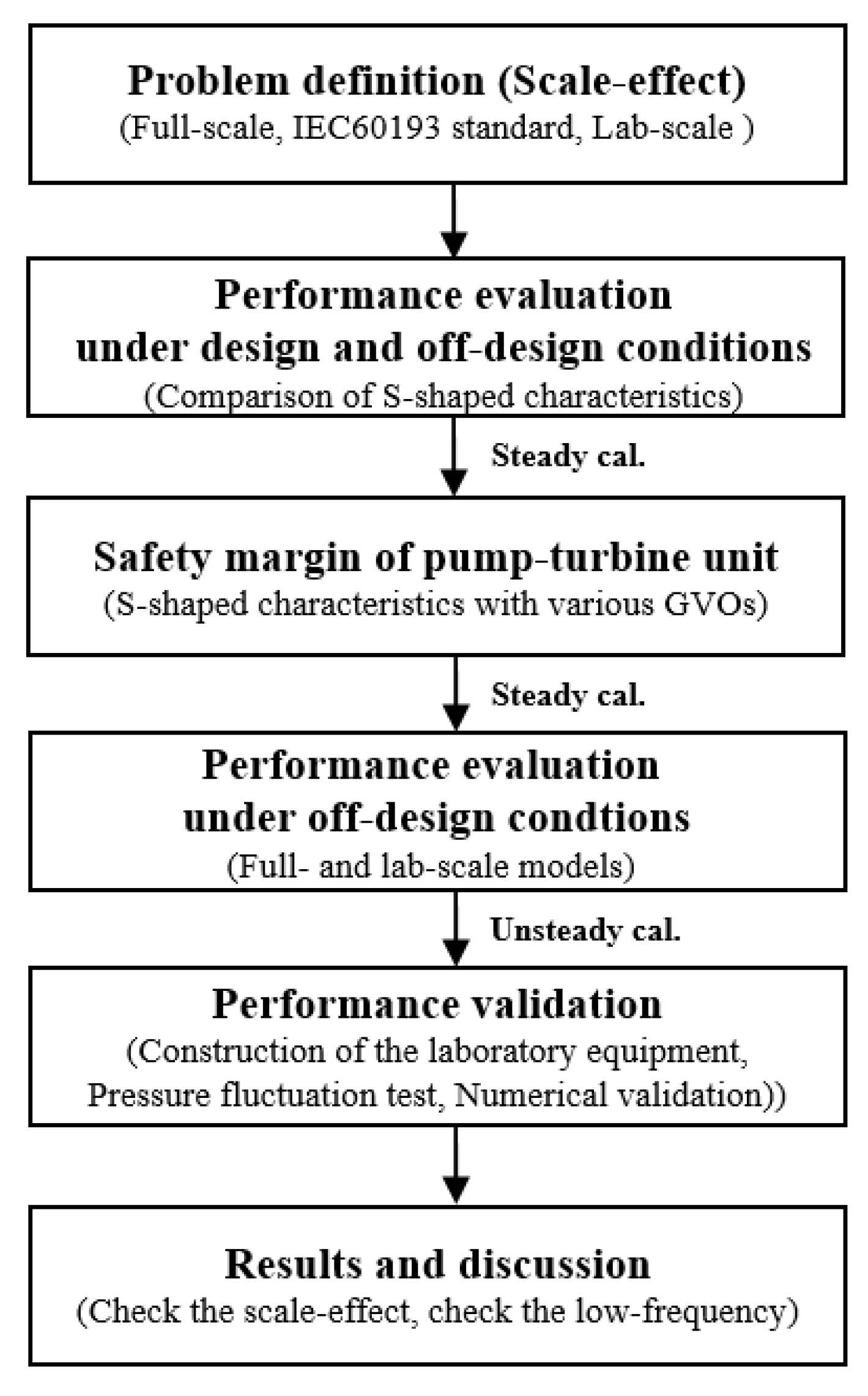
2. Research Procedure

Figure 1 shows the outline of the numerical analysis procedure. This research aimed to systematically investigate the scale effect on the S-shaped characteristics using commercial CFD packages and experiments. The geometry of the full-scale pump-turbine unit was initially studied in both generating and pumping modes [20,21]. Based on the established results, the laboratory-scale pump-turbine units were studied in the generating mode.

Figure 2 shows the research procedure concerning the analysis of performance characteristics of model scales in transition regions. First, S-shaped characteristics among model scales, such as full-, IEC60193 standard-, and laboratory-scale experiments, were compared to investigate the influence of the scale effect by solving steady Reynolds-averaged Navier–Stokes (RANS) equations. Using the scale-down function of ANSYS-CFX, the number of grids was kept the same, but the Reynolds number and a value of y+ were differently calculated because, depending on the scales, the applied flow rate and static pressure differ. Second, the laboratory-scale steady RANS equations were solved to investigate the safety margin for S-shaped characteristics. The GVO conditions with 8.5, 12.5, 17, 24, and 27 degrees were selected. Third, the full- and laboratory-scale unsteady RANS equations with the scale-adaptive simulation shear stress transport (SAS-SST) turbulence model were discretized to analyze pressure pulsation under optimal GVO conditions. Fourth, the predicted results were verified to the experimental results. The laboratory equipment was designed and manufactured by measuring the four-quadrant characteristic curve from the normal operating to the transition region. It was configured to measure the pressure pulsation characteristics, as well as the hydraulic performance, over time.

3. Numerical Modeling and Schemes

3.1. Governing Equations

Calculating the turbulent flow using CFD is much more complicated than the laminar flow. This is because of the always unsteady and three-dimensional characteristics of turbulent flow fields. Especially, a random, swirling three-dimensional vortex structure called eddy is created. In this study, the governing equations were discretized to investigate the characteristics of turbulent flow fields. For steady incompressible turbulent flows, the continuity and momentum are defined as follows:

$$\frac{\partial }{\partial x_j}\left(\rho u_j\right)=0$$

(1)

$$\frac{\partial }{\partial x_j}\left(\rho u_j{u}_i\right)=-\frac{\partial P}{\partial x_j}+\frac{\partial {\tau }_{ij}}{\partial x_j}$$

(2)

$${\tau }_{ij}=-\left(\begin{array}{ccc}\overline{u^{\prime }{}^2}& \overline{u^{\prime }{v}^{\prime }}& \overline{u^{\prime }{w}^{\prime }}\\ \overline{u^{\prime }{v}^{\prime }}& {\overline{u}}^{\prime }{}^2& \overline{v^{\prime }{w}^{\prime }}\\ \overline{u^{\prime }{w}^{\prime }}& \overline{v^{\prime }{w}^{\prime }}& u^{\prime }{}^2\end{array}\right).$$

(3)

On the right side of the equation, a term representing turbulent fluctuations is added. τ_ij is the specific Reynolds stress tensor, and the overbar represents the time average of the times components, and the prime represents the velocity component. Since Reynolds stresses are symmetrical, six additional endnotes were introduced. These new unknowns were modeled in various ways using turbulence models [22,23].

The most commonly used two-equation turbulence models in turbomachinery such as k-ε, k-ω, and k-ω based SST models that are added two transport equations [24,25]. This equation must be simultaneously solved with mass and linear momentum equations. Turbulence models emphasize that the equation is an approximate method that heavily relies on empirical constants. These models are calibrated by experimental data obtained from simple flow fields that isotropically attenuate downstream of the screen, such as direct numerical simulations, plate boundary layers, and shear layers. Unfortunately, none of the turbulence models are universal nor do they always lead to a physically correct solution.

As mentioned earlier, the two-equation model currently in use differs from the fundamentally accurate transport equation in that the exact equation of ε accounts for the dissipation scale, not the full scale. However, modeling the effect of the large-scale flow on the average flow is the ultimate goal of the two-equation model. A consistent approach was developed by Rotta to formulate the scale equation. Instead of the traditional method, Rotta formulated an accurate transport equation for the turbulent kinetic energy times the length scale, kL. Rotta’s equations represent large-scale turbulence, which can be the basis for modeling between terms [26,27]. Rotta derived the exact equation for kL from the Reynolds stress equation and with drastic surgery and standard closure approximation on the exact equation. The governing equations of the SAS-SST model are fully described in Menter and Egorov [28]. Using the method developed by Rotta, this model is based on the introduction of the von Karman length scale, L_vk, into the scale-determining equation of RANS turbulence models. Mentor and Egorov transformed the $\sqrt{k}L$ equation to the SST ω-equation using $\sqrt{k}L=1/C_{\mu }^{1/4}k/\omega$ and obtained the following SST ω-equation:

$$\frac{\partial \omega }{\partial t}+\frac{\partial }{\partial x_j}\left(U_j\omega \right) = \alpha \frac{\omega }{k}{G}_k-\beta {\omega }^2+Q_{SAS}+\frac{\partial }{\partial x_j}\left[\left(v+\frac{v_t}{{\sigma }_{\omega }}\right)\frac{\partial \omega }{\partial x_j}\right]+\left(1-F_1\right)\frac{2}{\omega {\sigma }_{\omega 2}}\frac{\partial k}{\partial x_i}\frac{\partial \omega }{\partial x_i}$$

(4)

$$G_k = -\overline{u_i{u}_j}\frac{\partial u_i}{\partial x_j}$$

(5)

$$Q_{SAS} = max\left[{\eta }_2\kappa S^2{\left(\frac{L}{L_{vK}}\right)}^2-C\frac{2\kappa }{{\sigma }_{\varphi }}max\left(\frac{1}{{\omega }^2}\frac{\partial \omega }{\partial x_j}\frac{\partial \omega }{\partial x_j}, \frac{1}{k^2}\frac{\partial k}{\partial x_j}\frac{\partial k}{\partial x_j}\right), 0\right]$$

(6)

$${\eta }_2 = 3.51, {\sigma }_{\varphi } = \frac{2}{3},C = 2, L_{vK} = \kappa \left|\frac{U^{\prime }}{U^{″}}\right|$$

where F₁ is the blending function to solve the free stream sensitivity problem of the ω-equation. L_vk plays an important role in determining the unsteady variation of the mean flow field. SAS-SST allows the resolution of the turbulent spectrum in unstable flow conditions, thereby leading to an LES-like simulation in the unsteady regions of the flow field.

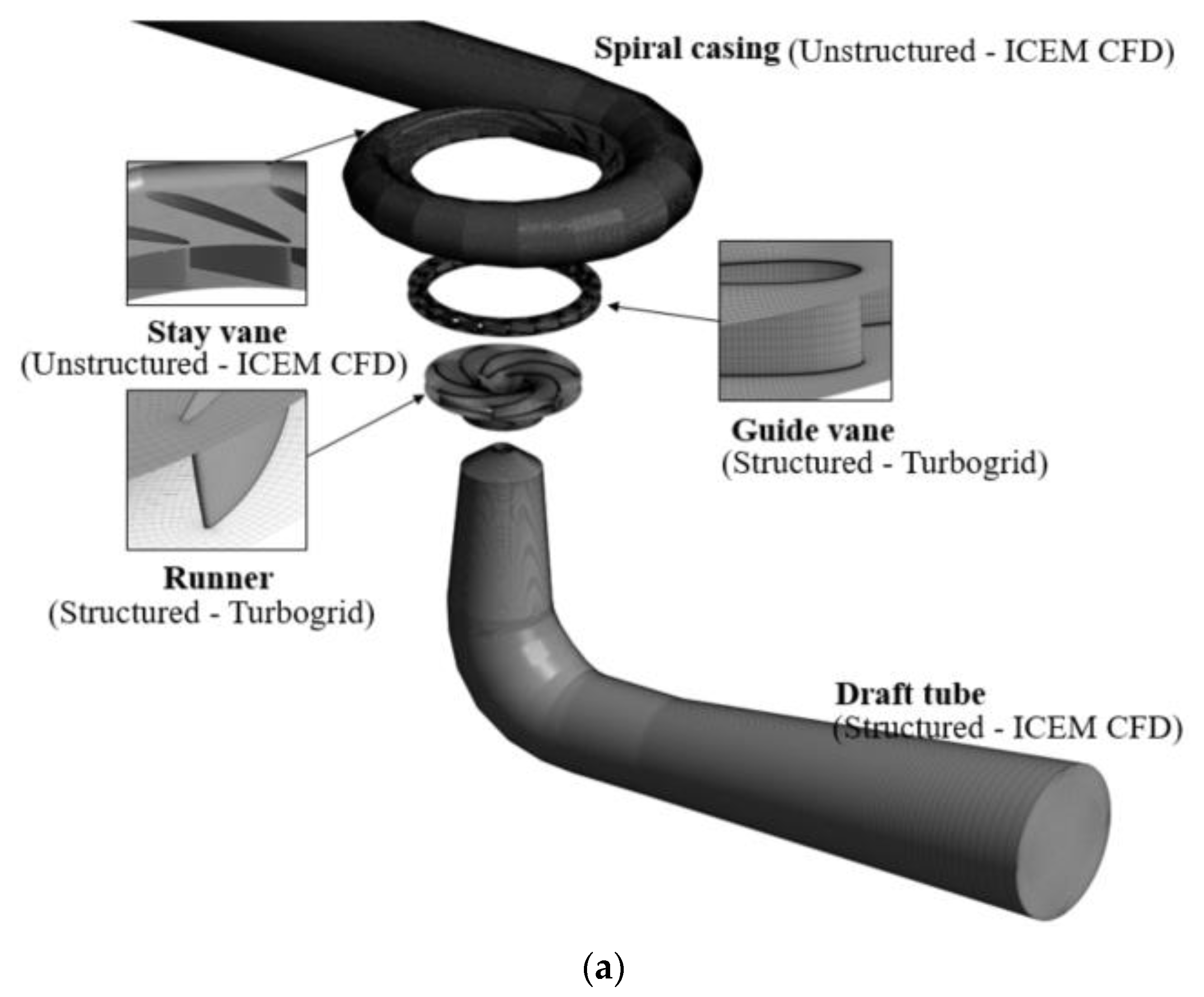
3.2. Computational Domain and Numerical Scheme

Figure 3 shows the geometrical structure and computational domain of the numerical calculation. The entire hybrid grid system (unstructured and structured grids) was meshed using ANSYS 19.2 (using BladeGen, TurboGrid, ICEM CFD) [29]. In the case of the full-scale model, to employ the high-Reynolds wall treatment method due to considering the computational time and cost, the first node point was kept at 30 ≤ y+ ≤ 300 within the logarithmic region. The runner and guide vane were refined to ensure that their y+ values remained less than 100. Besides, the y+ values of the stay vanes, spiral casings, and draft tubes were within the range ≈ 150–200. The number of nodes was 5.3, 6.6, 10.4, and 12.5 million, respectively [20]. In terms of the lower resource requirement and better convergence, the optimal node number was 10.4 million. In the case of the laboratory-scale model, since the diameter of the runner is relatively small, the grid can be densely positioned near the wall. Therefore, the SAS-SST turbulence model can be applied because it uses no wall function and directly analyzes the node point near the wall when it is below y+ ≈ 1. The detailed information and boundary conditions regarding the first to fourth steps are shown in

Table 1. Number of nodes for the main components.

	Full-Scale (1)	IEC60193 Standard-Scale (1/11)	Laboratory-Scale (1/20)
Reference diameter [m]	2.77	0.25	0.1385
Number of nodes	1.0 × 107	1.0 × 107	1.0 × 107
Value of y+ (RV/GV/SV/SP/DT)	y+ ≈ 100 (RV/GV) y+ ≈ 150 (SV/SP/DT)	y+ ≈ 2 (RV/GV) y+ ≈ 2 (SV/SP/DT)	y+ ≈ 1 (RV/GV) y+ ≈ 1 (SV/SP/DT)
Reynolds number	1.4 × 108	7.2 × 106	3.6 × 105
Turbulence model	SST high-Reynolds number	SST low-Reynolds number	SST low-Reynolds Number

,

Table 2. Boundary conditions for predicting S-shaped characteristics among model scales.

Turbineand TurbineBrake
Inlet (spiral casing)	Total pressure (energy coefficient, 0.117)
Outlet (draft tube)	Mass flow rate (1.0QBEP, 0.5QBEP, 0.3QBEP, 0.1QBEP)
Reverse pump (reverse flow direction)
Inlet (draft tube)	Average static pressure (energy coefficient, 0.117)
Outlet (spiral casing)	Mass flow rate (0.2QBEP, 0.1QBEP)
Speed factor	2.91 (360, 1200, 1800 rev/min)
Discharge factor	0.065 (89, 0.21, 0.054 m3/s)
Turbulence model	SST high-Reynolds number (full-scale) SST low-Reynolds number (IEC60193 standard-scale, laboratory-scale)
Guide vane opening	21.5°
Interface condition	Stage-average
Calculation type	Steady-state calculation

,

Table 3. Boundary conditions for predicting safety margin for S-shaped characteristics.

Turbineand TurbineBrake
Inlet (spiral casing)	Total pressure (energy coefficient, 0.117)
Outlet (draft tube)	Mass flow rate (1.0QBEP,0.5QBEP,0.3QBEP,0.1QBEP)
Reverse pump (reverse flow direction)
Inlet (draft tube)	Average static pressure (energy coefficient, 0.117)
Outlet (spiral casing)	Mass flow rate (0.2QBEP, 0.1QBEP)
Speed factor	2.91 (1800 rev/min)
Discharge factor	0.065 (0.054 m3/s)
Turbulence model	SST low-Reynolds number
Guide vane opening	8.5°, 12.5°, 17°, 21.5°, 24°, 27°
Interface condition	Stage-average
Calculation type	Steady-state calculation

and

Table 4. Boundary conditions for unsteady-state calculation predicting the transition region.

Turbine and Turbine Brake
Guide vane opening	21.5°
Total time	1.667 [s]–10 revolutions
Time step	0.00046305 [s], 1°
Initial condition	Result of steady-state calculation
Turbulence model	SAS-SST model
Interface condition	Transient rotor stator
Calculation type	Unsteady-state calculation

[30]. The steady and unsteady flows were calculated until the simulation reached the required root-mean-square residual (between 1.0 × 10⁻⁵ and 1.0 × 10⁻⁶). The simulation was performed on a 32-core dual-processor Xeon (2.80 GHz) central processing unit. The calculation was divided into 32 tasks. Under the steady-state condition, the calculation time was approximately 8 h. Under the unsteady-state condition, the time step was set to 0.00046305 s. The solution was acquired in 3600 time steps for 1.668 s. The calculation time was approximately 156 h.

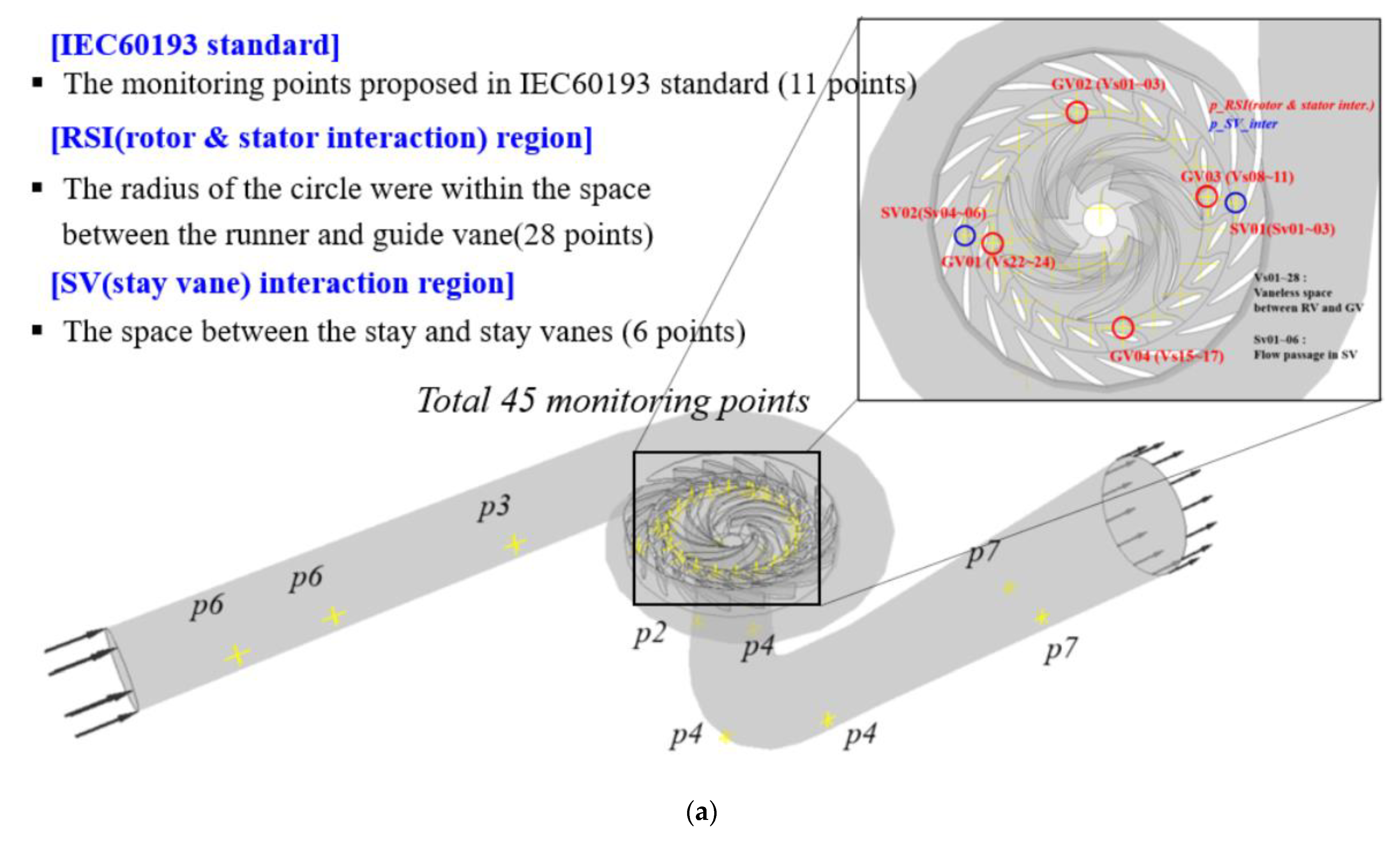
3.3. Schematic Diagram of Monitoring Points

Figure 4 shows monitoring points in the computational domain and experimental setup. The pressure-monitoring points were used to understand the propagation and pulsation of unsteady pressure characteristics. As shown in Figure 4a, the 11 measurement points suggested in IEC60193 and the considered 28 monitoring points located were within the space between the rotating and stationery domains. Furthermore, the six monitoring points were located between the stay and stay vanes. It is known that the dominant pressure pulsation occurs in the vaneless space [31]. Since comparing the pressure characteristics induced by the internal flow field between the full- and laboratory-scale models was the purpose, the six representative monitoring points were selected for the location of the piezoelectric sensor in the experimental equipment.

4. Experimental Methods

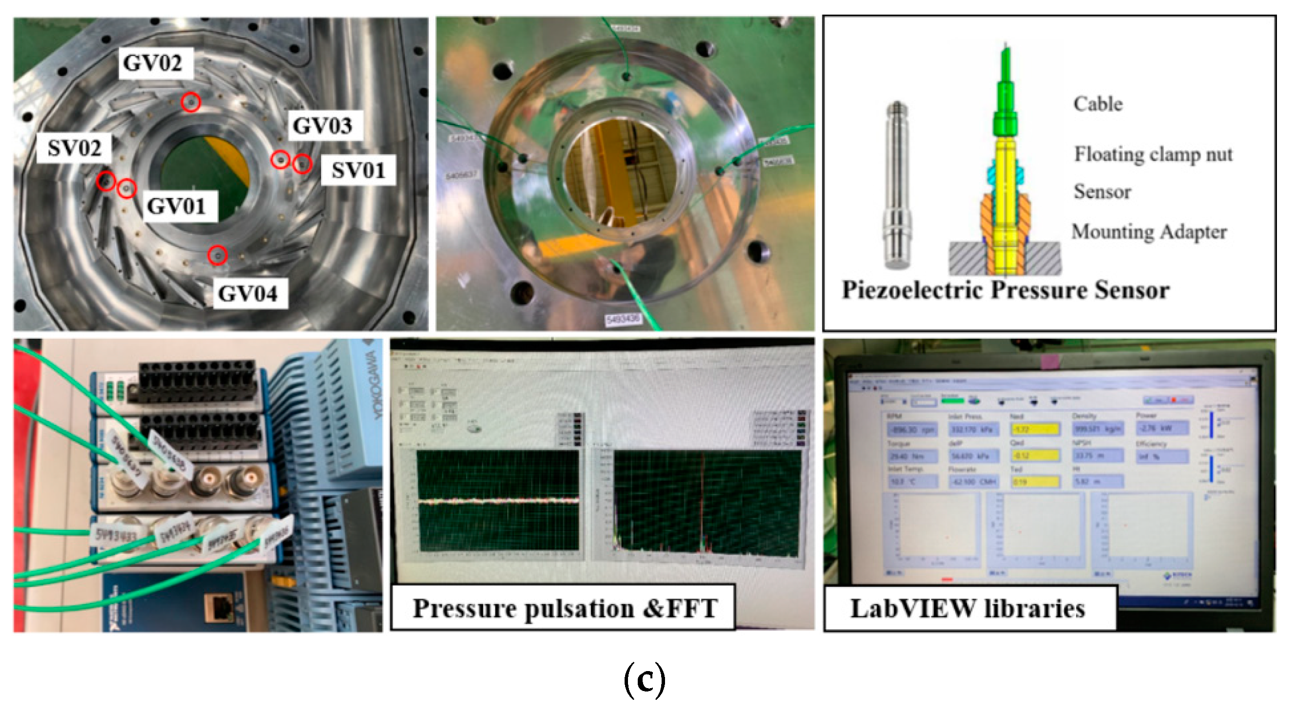
4.1. Experimental Methods of the Full-Scale Model

The full-scale model was installed to conduct a performance test on a real site. The experimental data was measured based on the IEC60041 standards, which is about field acceptance tests to determine the hydraulic performance of pump-turbines. Some conditions (lower flow rate) could not be applied and performed due to the real-site pump turbine; therefore, the test results were only executed up to 50% of the test load. The basic performance test did not provide detailed results on pressure pulsation. The performance measurement approach was employed by the thermodynamic method [32]. The thermodynamic method results of applying the principle of energy conservation to the transfer of energy between water and the runner. This method allows direct measurement of the specific mechanical energy. The uncertainties for power and efficiency were ±1.14% and ±0.91%. The test condition at each point was determined for 5 min after 5–10 min of load settling time. The scan time interval is 20 Hz, and data was collected by a PC-based acquisition system.

4.2. Experimental Methods of the Laboratory-Scale Model

The laboratory-scale model was installed to perform a validation test on the Korea Institute of Industrial Technology. As shown in Figure 5, the laboratory equipment was designed and manufactured for measuring the four-quadrant characteristic curve from the normal operating to the transition region. Experimental analysis was performed in only one quadrant, but experiments were performed on the four-quadrant to utilize the numerical validation in future work. The experimental data was measured based on the standards and test methods of IEC60193 and was certified by the Korea Testing Laboratory. The temperature and pressure at the inlet and outlet, and the rotational speed and torque of the runner were measured, and through the valve control, the flow through the flowmeter was unified in a constant direction. Especially, the four-way valve was configured to maintain the same direction (forward to the flow meter) with the flow at various operating conditions and simplify the structure of the piping. The maximum allowed standard deviation of nominal value for the differential pressure and rotational speed was within ±0.05%, and absolute pressure was within ±0.1%, and flow rate and torque were within ±0.2%. Thus, the sensitivity of the piezoelectric pressure was 3333 mV/bar. The test condition at each point was determined for 20 points after 1 min of load settling time. A data acquisition (DAQ) system collected and processed the data output from this measuring equipment and implemented it to enable real-time monitoring using LabVIEW software. The DAQ system was also configured to control valves and inverters to facilitate performance testing.

5. Results and Discussion

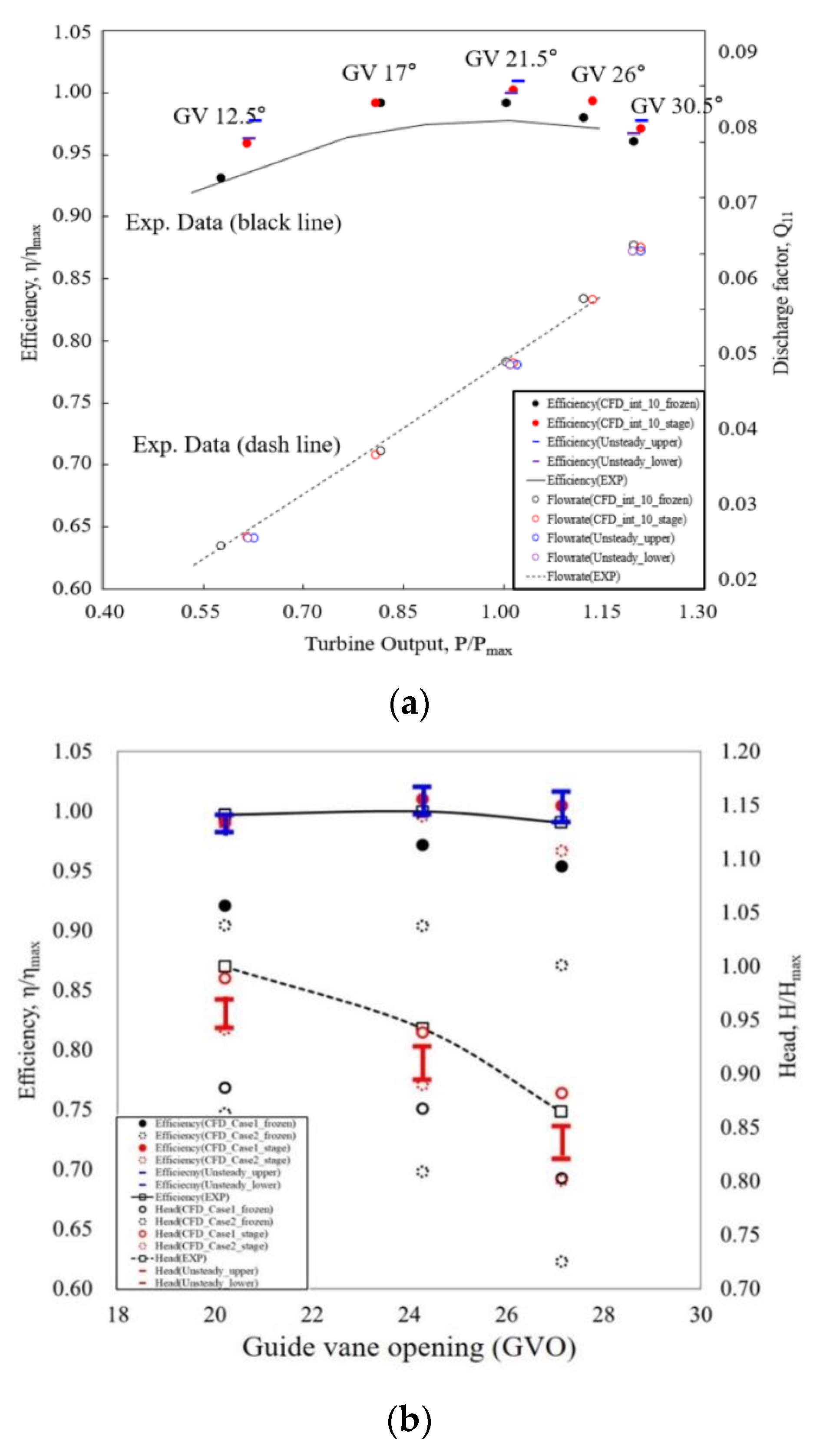
5.1. Validation of Numerical Results

In case of the full-scale model, the numerical validation is hard to perform under the off-design conditions as aforementioned in Chapter 4. Therefore, the steady and unsteady-state simulations were conducted under an optimal condition with various guide vane openings (GVOs). In the turbine mode, the GVO condition was varied as 12.5°, 17°, 21.5°, 26°, and 30°. In the pump mode, the GVO condition was varied as 20°, 24°, and 27°. A comparison of performance characteristics is shown in Figure 6. For both generating and pumping modes, the computational results for the transient rotor-stator method (interface method of the unsteady-state) were well-matched with the experimental data, and the trend has similarities with the stage-average method (interface method of the steady-state). In the case of the laboratory-scale model, the equipment was designed and manufactured for measuring the four-quadrant characteristic curve from the normal operating to the transition region. Experimental analysis was performed in only one quadrant, but experiments were performed on the four-quadrant to utilize the numerical validation in future work. Furthermore, the magnitude of and variation in the unsteady pressure fluctuation were collected and processed. Figure 7 shows the numerically simulated and experimentally determined four-quadrant characteristic curves with various GVOs.

Table 5. Validation of numerical simulation results at guide vane opening (GVO) = 21.5°.

Operating Point	Factor	Experiments	Simulation (Steady-State)	Simulation (Steady State)
Normal operating (Q/Qd = 1.0)	ned	1.5672	1.6234	1.6263
	Qed	0.1697	0.1759	0.1762
	Ted	0.0952	0.0986	0.0978
Half-load condition (Q/Qd = 0.5)	ned	2.0303	1.9979	2.0217
	Qed	0.1107	0.1083	0.1095
	Ted	0.0146	0.0217	0.0217
Runaway condition (Q/Qd = 0.3)	ned	2.0332	1.9368	1.9811
	Qed	0.0645	0.0630	0.0644
	Ted	−0.0067	0.0021	0.0033
Low-discharge condition (Q/Qd = 0.1)	ned	1.9481	1.8797	1.8796
	Qed	0.0211	0.0204	0.0203
	Ted	−0.0276	−0.0134	−0.0145

presents the difference between N_ed, Q_ed, and T_ed values derived through experimental and numerical analysis (steady- and unsteady-state) results. It is found that the numerical analysis and the tendency of the experiment well-matched in the overall operating and transition region with very high reliability (within 4%).

5.2. Predicting S-Shaped Characteristics between Model Scales

In order to achieve good hydraulic similarity, it is necessary to define the minimum value for the model size and test parameters [7]. Based on the IEC60193 standard, the reference diameters, Reynolds number, Froude number, and specific hydraulic energy between the reduced-scales are 0.25 [m], 0.1385 [m] and 7.2 × 10⁻⁶, 3.6 × 10⁻⁵ and 6.41 × 10⁻⁷, 8.61 × 10⁻⁷ and 373 [J/kg], 255 [J/kg], respectively. The S-shaped characteristics between IEC60193 standard- and laboratory-scale models were compared to investigate the influence of the scale effect, as shown in

Table 6. Comparison of the S-shaped characteristics of model scales at 21.5° GVO.

Operating Point	Factor	IEC60193 Standard-Scale (Steady State)	Laboratory-Scale (Steady State)
Normal operating condition	ned	1.6282	1.6234
	Qed	0.1765	0.1759
	Ted	0.0998	0.0986
Half-load condition	ned	2.0030	1.9979
	Qed	0.1086	0.1083
	Ted	0.0222	0.0217
Runaway condition	ned	1.9340	1.9368
	Qed	0.0630	0.0630
	Ted	0.0021	0.0021
Low-discharge condition	ned	1.8822	1.8797
	Qed	0.0204	0.0204
	Ted	−0.0131	−0.0134
Reverse pump condition	Ned	1.9065	1.9199
	Qed	−0.0208	−0.0209
	Ted	−0.0423	−0.0429

. In the overall transition operation area, the reduced models showed S-shaped characteristic results, as shown in Figure 8. The analysis results were maintained at a similar level. In the case of the laboratory-scale model, the model size is smaller than the minimum standard of IEC60193, but the steady-state analysis showed a highly similar value. The maximum allowed standard deviation of nominal value for the differential pressure and rotational speed was within ±1%. Furthermore, the difference in hydraulic efficiencies was within 1% under the overall operating conditions. Since the scale effect was not dominant, a laboratory-scale model was used as a reduced model instead of the IEC60193 standard-scale. Therefore, the full- and laboratory-scale models were compared by using unsteady-state analysis.

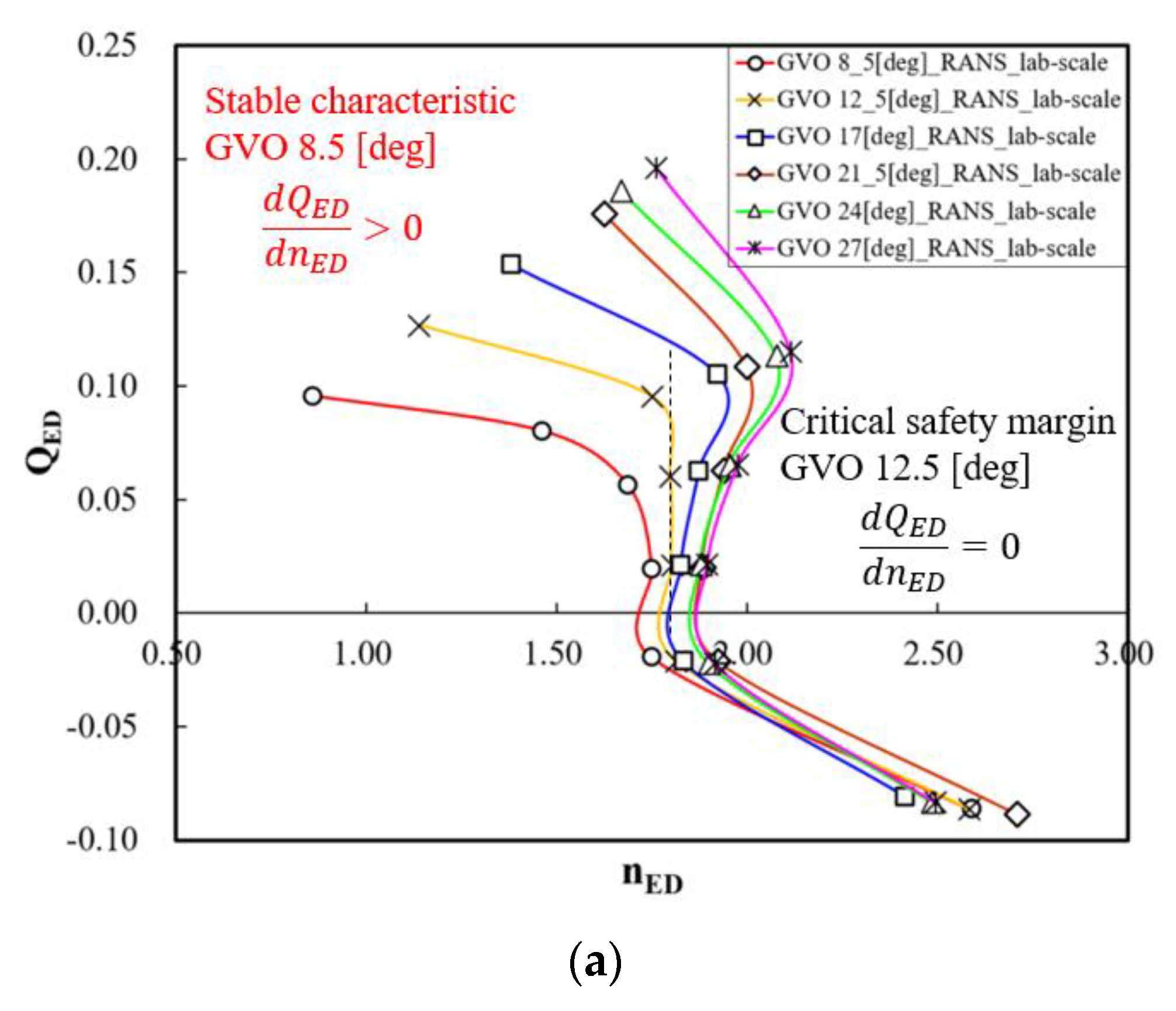
5.3. Safety Margin of S-Shaped Characteristics

A sufficient safety margin of the S-shaped characteristics must be provided to avoid start-up/load rejection and change in operating modes. Therefore, the steady RANS equations were discretized to investigate the safety margin prior to performing the unsteady-state simulation. As shown in Figure 9, the GVO condition was varied as 8.5°, 12.5°, 17°, 21.5°, 24°, and 27°. The positive slope of the S-curve tended to increase as the GVO increased because of the interaction between the variation of guide vane angle and the runner blade angle. In the steady-state analysis, 12.5° GVO was determined as the critical GVO, and 8.5° GVO stabilized the S-shaped characteristic under close to the speed-no load condition.

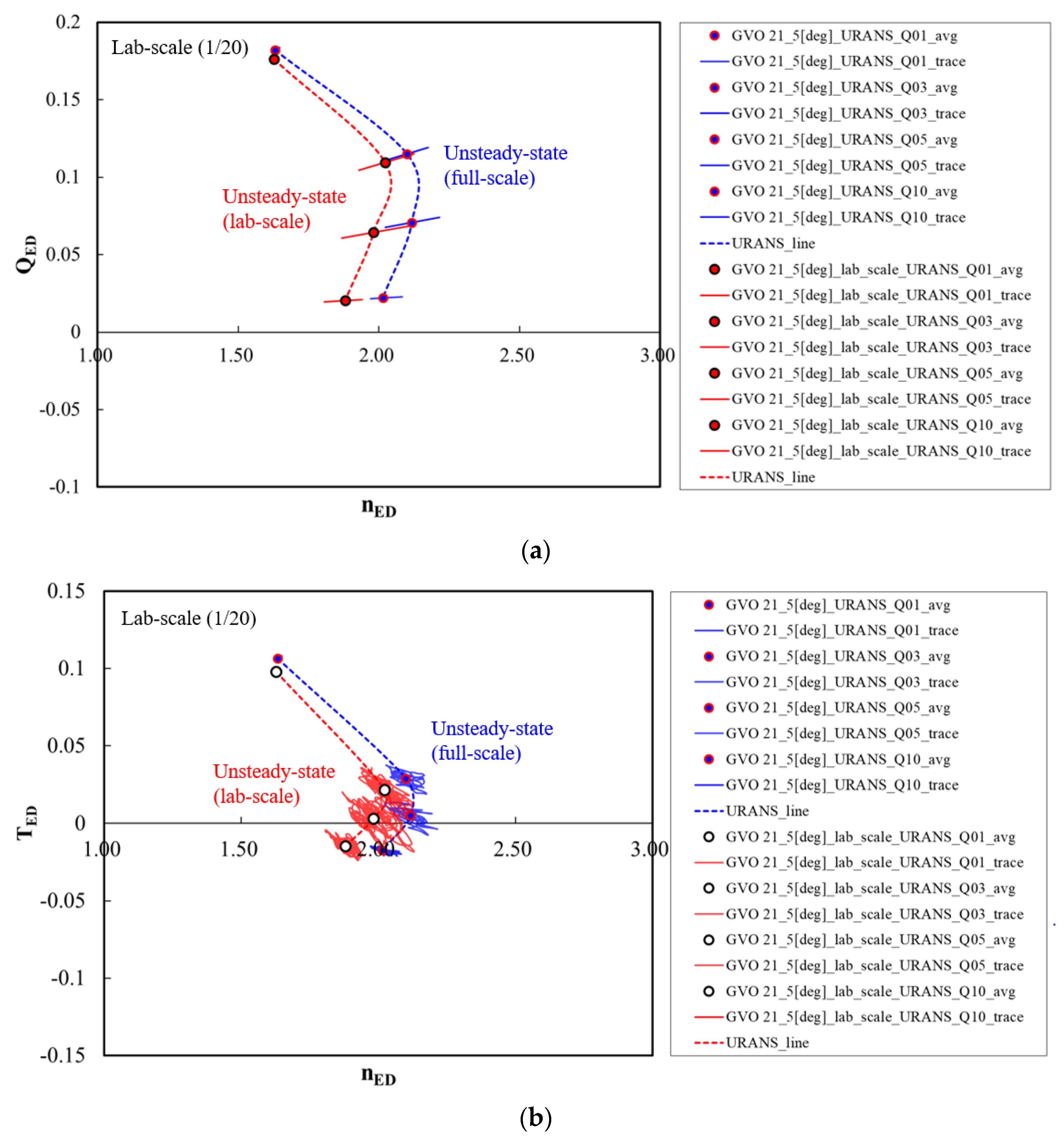
5.4. Comparison of Unsteady S-Shaped Characteristics

Table 7. Unsteady-state results of full- and laboratory-scale models at 21.5$°$ GVO.

Operating Point	Factor	Full-Scale (Averaged Value)	Laboratory-Scale (Averaged Value)
Normal operating condition	ned	1.6317	1.6263
	Qed	0.1819	0.1762
	Ted	0.1063	0.0978
Half-load condition	ned	2.1001	2.0217
	Qed	0.1150	0.1095
	Ted	0.0287	0.0217
Runaway condition	ned	2.1201	1.9811
	Qed	0.0708	0.0644
	Ted	0.0052	0.0033
Low-discharge condition	ned	2.0148	1.8796
	Qed	0.0221	0.0203
	Ted	−0.0174	−0.0145

and Figure 10 show the results of the unsteady-state analyses of the full- and laboratory-scale models, respectively. For the results of both models, similar normalized values were predicted under normal operating conditions because the scale effect was not dominant. However, it is confirmed that the difference in the averaged-value increases as it went toward the transient region, and the variation of the speed and flow factors increases. The variations of pressure pulsation tended to peak and then decrease again in runaway conditions. Depending on the range of time and pulsation, the two models may be located at the same dimensionless value, or else the difference can be seen to be substantially greater. The slope of the speed and flow factors was similar for each operating point, as the function of the slope consists of mass flow rate, rotational speed, and reference diameter. The three parameters are fixed because the rotational speed and reference diameter are constraints according to the law of similarity. However, the value of the head varies over time due to the flow blockage phenomena. Therefore, the averaged-value of each operating point is offset to a certain level.

5.5. Unsteady Pressure and Internal Flow-Field Characteristics

Figure 11 presents the time records of pressure fluctuation at representative monitoring points under the speed-no load condition. There was a difference in the resolution of the pressure fluctuation between the full- and laboratory-scale models because the rotational speed of the laboratory-scale model was five times faster than that of the full-scale model. Four sensors (GV01-04) were installed in the vaneless space, and two sensors were placed in the passage between the stay vanes. The x-axis represents the time histories along 5–10 revolutions, and the y-axis represents the normalized pressure coefficient. The pressure coefficient fluctuation is defined as follows:

$$\widetilde{C_p} = \frac{p-\overline{p}}{\rho gH}.$$

(7)

Figure 11a shows the pressure pulsation pattern developed during movement from the stay vane to vaneless space. The variation in pressure fluctuation is large, but it is intuitively predictable that there is no rotational stall due to the lack of periodicity in the pressure pulsation. As obtained in the results, the variation in pressure fluctuation was notable in the laboratory-scale model, while the form of pressure fluctuation was found to be periodic. Therefore, the occurrence of a rotating stall (RS) could be intuitively checked through the periodicity of the pressure fluctuations. Accordingly, a more detailed analysis was performed in the vaneless space along the circumferential direction.

Figure 12 presents the time records of pressure fluctuations at all monitoring points in the vaneless space under normal and transition regions. The x-axis represents the time histories along 5–10 revolutions, the y-axis represents the monitoring points placed at equal intervals in the circumferential, and the z-axis represents the normalized pressure coefficient. The variation is not dominant under normal operating conditions. Under the half-load condition, undesired pressure fluctuations with no periodic pattern were induced by flow separation. Under the runaway and low-discharge conditions, periodic patterns were visible. In the transition region, the origins of the RS develop at a runaway condition (speed-no load), and is fully developed at the reduction in the discharge (low-discharge); then, it decreases near the zero-discharge condition. For a more detailed investigation of periodicity, the original signal was input to a low-pass filter, and the original and filtered signals were compared. As shown in Figure 13, the time histories of the original and low-pass filtered signals were represented at all monitoring points in the vaneless space under the runaway condition. Both the original and low-pass-filtered signals were periodic and moved by a distance of one phase difference from Vs09 to Vs23. Using the low-pass-filtered signal, the periodicity of the original signals was visible. In addition, the rotational speed of the RS could be estimated from the slope of the line connecting the pressure peaks in two consecutive runner revolutions. In this paper, rather than using the equation of the reference, the rotational speed of the RS was calculated through the fast Fourier transform (FFT) technique. The FFT provides a more detailed data processing, revealing the characteristic frequency of the RS, the blade-passing frequency (BPF), and the amplitude of the unsteady vortex signals. A time-frequency analysis of the transient pressure pulsations at the monitoring points was calculated through the commercial software. The Fourier transform of the numerical computation was done with an FFT algorithm in Origin Pro 2019b software [33]. Using the unsteady-state analysis, the 2,048 sampling points were acquired at the monitoring position. The Fourier transform of the experiment was done with an FFT algorithm in LabVIEW [34]. The power spectrum filter with a sampling speed is 25.6 kHz was calculated using a Hanning window. Figure 14 shows the comparison of the frequency spectra obtained by the FFT between the full- and laboratory-scale models. Along the x-axis, f/f_n denotes the non-dimensional frequency of the signals normalized by the runner rotating frequency. As mentioned earlier, there is no evidence about the RS in the full-scale model. Therefore, the frequency spectra were remarkable only at f/f_n = 7.0, 14.0, and 21.0 (representing the first, second, and third BPF harmonics). In the case of the laboratory-scale model, the frequency spectra were remarkable at f/f_n = 0.6 and 1.2 (representing the RS) and f/f_n = 7.0, 14.0, and 21.0 (representing the first, second, and third BPF harmonics, respectively). These results represent an RS with a frequency propagation around 60% of the runner speed at the runaway condition. The overall numerical and experimental frequency spectra results were well-matched, except in the low-frequency region where the numerical analysis results were overestimated. It is confirmed that the results of numerical analysis over-predicted the values compared to the experiments. In f/f_n = 0.6, the result of the numerical analysis showed a value corresponding to approximately 0.09–0.16 at the positions where the phase difference was 90 degrees in the vaneless space. The result of the experiment showed a value corresponding to approximately 0.04–0.05 in the same positions. In f/f_n = 0.6, the result of the numerical analysis showed a value corresponding to approximately 0.07 at a position where the phase difference was 180 degrees different from the passage between stay vanes. The result of the experiment showed a value corresponding to approximately 0.03–0.04 in the same positions. In the passage between stay vanes, the value of the low-frequency region was higher than the first BPF and had the most dominant value. The numerical analysis derives a specific value in time from the given boundary condition, but the output of the experimental result is widely variable and includes the effects of noise from the entire system.

The RS cell periodically rotates in the same direction as the runner with a rotating frequency that is about 50–70% of the sub-synchronous frequency, depending on the geometrical information and specific speed. The results of this study are consistent with others conducted on RS frequency through numerical and experimental studies [4,12,35].

The internal flow characteristics were analyzed based on the comparatively verified results. In general, there are two ways to control the flow in turbine mode: By adjusting the guide vane and by controlling the valves fixed at the guide vane. The latter method is used in this study. From a theoretical point of view, the absolute flow angle has a constant value. At the design flow rate, the relative flow velocity angle, β₁, is large, and the incidence angle of the fluid passing through the leading edge is the minimum. At low-discharge conditions, the relative flow angle becomes smaller than the design flow rate due to the decrease in the meridional velocity, and the incidence angle increases further.

Figure 15 shows the comparison of the instantaneous radial velocity contours and vectors in the vaneless space between the full- and laboratory-scale models, showing the detailed internal flow field at the interface. Under the normal operating condition of both models, the flow direction in the turbine mode was from the guide vane to the runner. On the other hand, the backflow became prominent under the runaway condition. Based on the maximum radial velocity, the magnitude differed by four times between the models, and the size of the vector compared to the dimensional size of the computational domain was stronger in the case of the laboratory-scale model. Figure 16 shows the comparison of the instantaneous velocity streamlines with forward and backward directions in the runner between the full- and laboratory-scale models. This figure reveals the detailed three-dimensional internal flow field in the runner. As the flow rate decreased, the backflow became more prominent, and the flow blockage and consequent backward flow appeared under the runaway condition.

Figure 17 represents the time history and representative velocity streamlines and contours on the runner mid-span section. As measuring the flow pattern becomes difficult over time, the internal flow showed no periodic pattern. The behavior in each passage was identified through internal flow-field analysis. Therefore, the flow rate of the runner at the inlet and outlet and the blade-loading curve were quantitatively analyzed in each channel at the last time step (selected as the representative time).

Brennen [36] explained the schematic of the mechanism of the RS, as shown in Figure 18. If channel “B” is stalled, a separated wake is generated, developing the blockage phenomenon within the passage. Therefore, it tends to turn the flow from the flow blockage, increasing the incidence angle on blade “a” and decreasing the incidence angle on blade “c.” Consequently, channel “A” tends to be stalled, while the existing stall in channel “B” or “C” tends to recover. Based on the mechanism mentioned in the literature, Figure 19 and Figure 20 show a comparison of the blade-loading distribution and normalized flow rate of runner channels between the models. In the case of the full-scale model (Figure 19a and Figure 20a), the blade-loading distribution mostly showed a negative pattern, indicating that the deflected flow from the flow blockage increased the incidence angle of the leading edge. As a result of checking the flow rate in and out of each flow passage, there was no RS, so the internal flow field was not completely blocked. According to whether the pattern of the normalized flow rate was relatively lower or higher than the average value in each blade, the form of the blade-loading distribution was represented. In the case of the laboratory-scale model (Figure 19b and Figure 20b), the evidence of an RS was found through FFT analysis. Some blade-loading distributions showed a positive shape, whereas the others showed a negative shape. On blades 1 and 7, the leading edge was positively shaped, whereas the trailing edge showed a shape in the reverse pump. As the result of checking the flow rate in and out of each flow passage, stalling in passages 1 and 7 caused the complete blockage of the internal flow field. Next, the characteristics of the passage adjacent to the stalled passage were investigated. On blade 6 in passage 6, the incidence angle decreased as the flow recovered from its stalled state. On blade 2 in passage 2, the incidence angle tended to increase as the flow was deflected from the flow blockage. In passages 3, 4, and 5, the incidence angle increased, and the flow was partially blocked.

$${\delta }_{ref} = \frac{1-{\eta }_{h opt M}}{\left[{\left(\frac{R{e}_{ref}}{R{e}_{opt M}}\right)}^{0.16}+\frac{1-V_{ref}}{V_{ref}}\right]}$$

(8)

$${\left(\mathsf{\Delta }{\eta }_h\right)}_{M^{*}\to P} = {\delta }_{ref}\left[{\left(\frac{R{e}_{ref}}{R{e}_{M^{*}}}\right)}^{0.16}-{\left(\frac{R{e}_{ref}}{R{e}_P}\right)}^{0.16}\right]$$

(9)

Finally, Figure 21 shows the efficiency change in hydraulically similar operating conditions having different Reynolds numbers (A and B). Based on the formula,

Table 8. Comparison of numerical results and application of tolerances for full- and laboratory-scale models.

(Δηh)M*→P	δref	Vref	Reref	ReoptM	ReP	ReM*	ηhoptM
0.0323	0.051579	0.7	7,000,000	1,800,682	144,054,539	1,800,682	0.9138

shows the comparison of results and application of tolerances for each model and prototype (laboratory- and full-scale models). The numerical results obtained by calculating the hydraulic efficiency of the full- and laboratory-scale models were 95.15% and 91.38%, respectively. Based on the results of the scale-down model, the value calculated by predicting the hydraulic efficiency of the full-scale model by applying it to the formula was 94.61% [7]. The scale-up effect between the models was found to be about 3.2%. The difference between the result calculated through numerical analysis and the value predicted through the calculation formula was 0.54%, verifying the reliability of the results.

6. Conclusions

This paper performed a comparative study of the scale effect on the S-shaped characteristics of a pump-turbine unit. The main conclusions are summarized below:

• The S-shaped characteristics between model scales were compared to investigate the influence of the scale effect. For the results of both models, similar normalized values were predicted under normal operating conditions because the scale effect was not dominant. However, it is confirmed that the difference in the averaged-value increases as it went toward the transient region, and the variation of the speed and flow factors increases. The variations of pressure pulsation tended to peak and then decrease again in runaway conditions. Depending on the range of time and pulsation, the two models may be located at the same dimensionless value, or else the difference can be seen to be substantially greater. The slope of the speed and flow factors was similar for each operating point, as the function of the slope consists of mass flow rate, rotational speed, and reference diameter. The value of the head varies over time due to the flow blockage phenomena. Therefore, the averaged-value of each operating point is offset to a certain level.
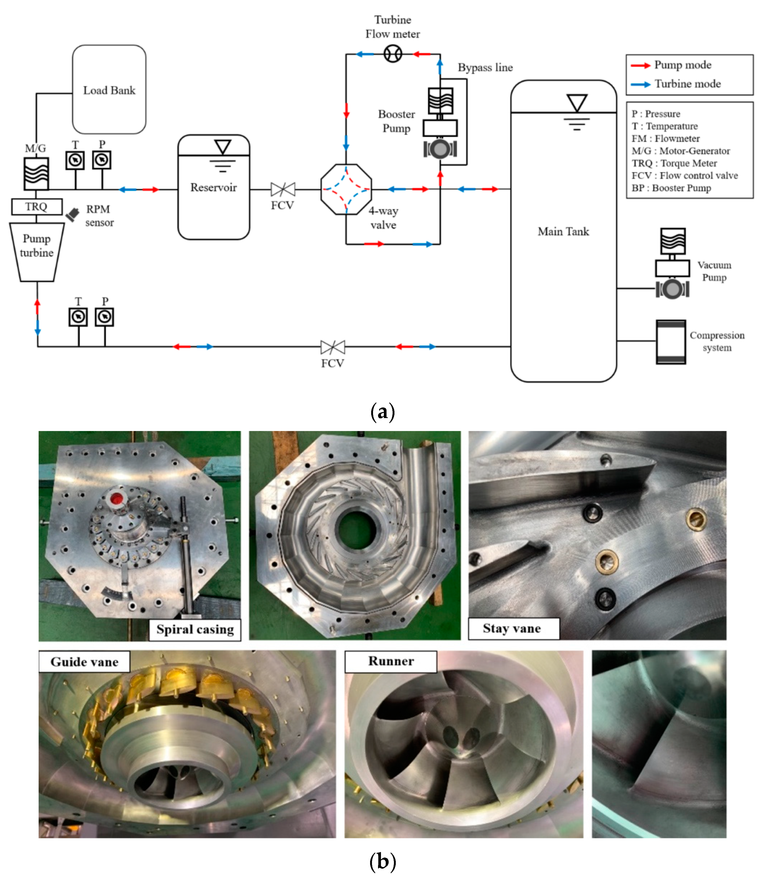
• The numerical result was validated in comparison with experimental results. In the experiment of the full-scale model, transition conditions were difficult to perform in detail; therefore, steady and unsteady simulations were conducted under an optimal condition with various GVOs. The laboratory equipment was designed and manufactured for measuring the four-quadrant characteristic curve from the normal operating to the transition region. The numerical and experimental tendencies were well-matched in the overall operating and transition region. After comparing the values, the reliability of the numerical analysis was determined within 4%.
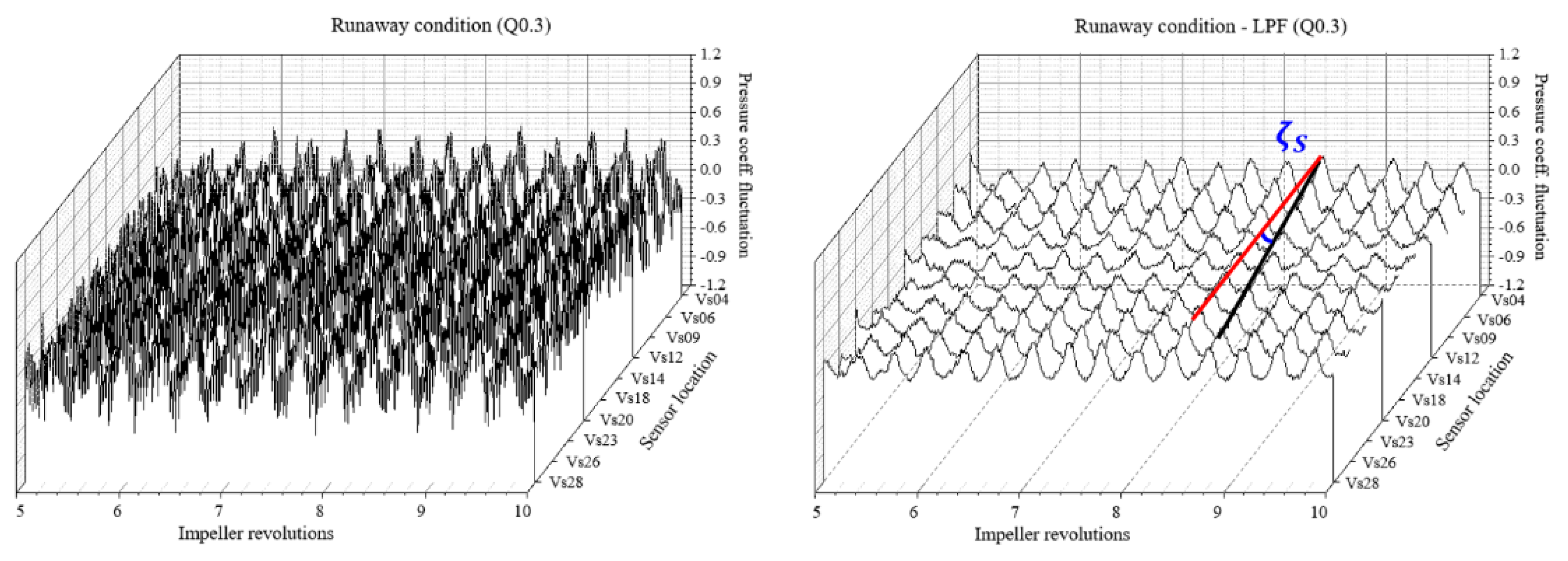
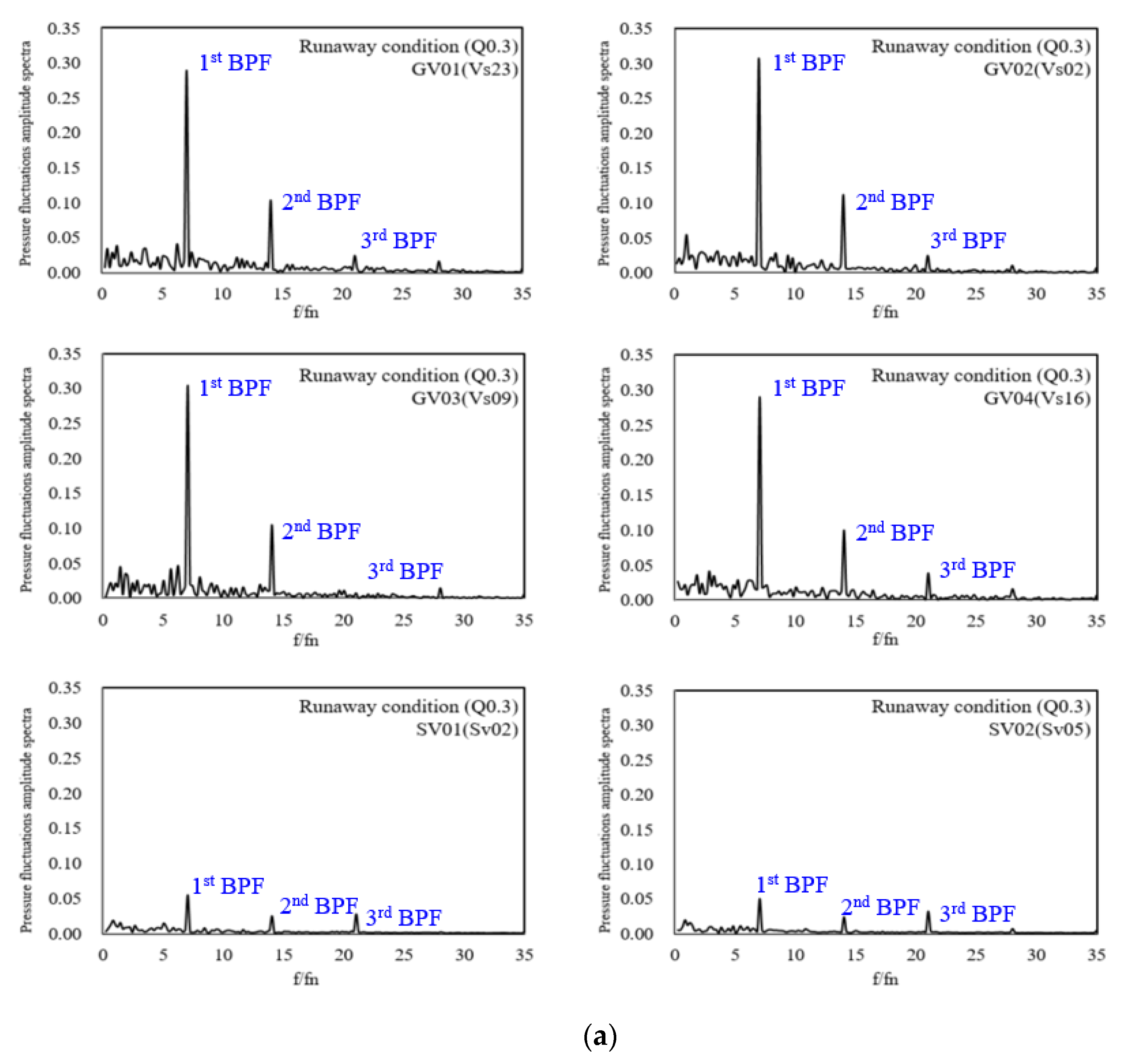
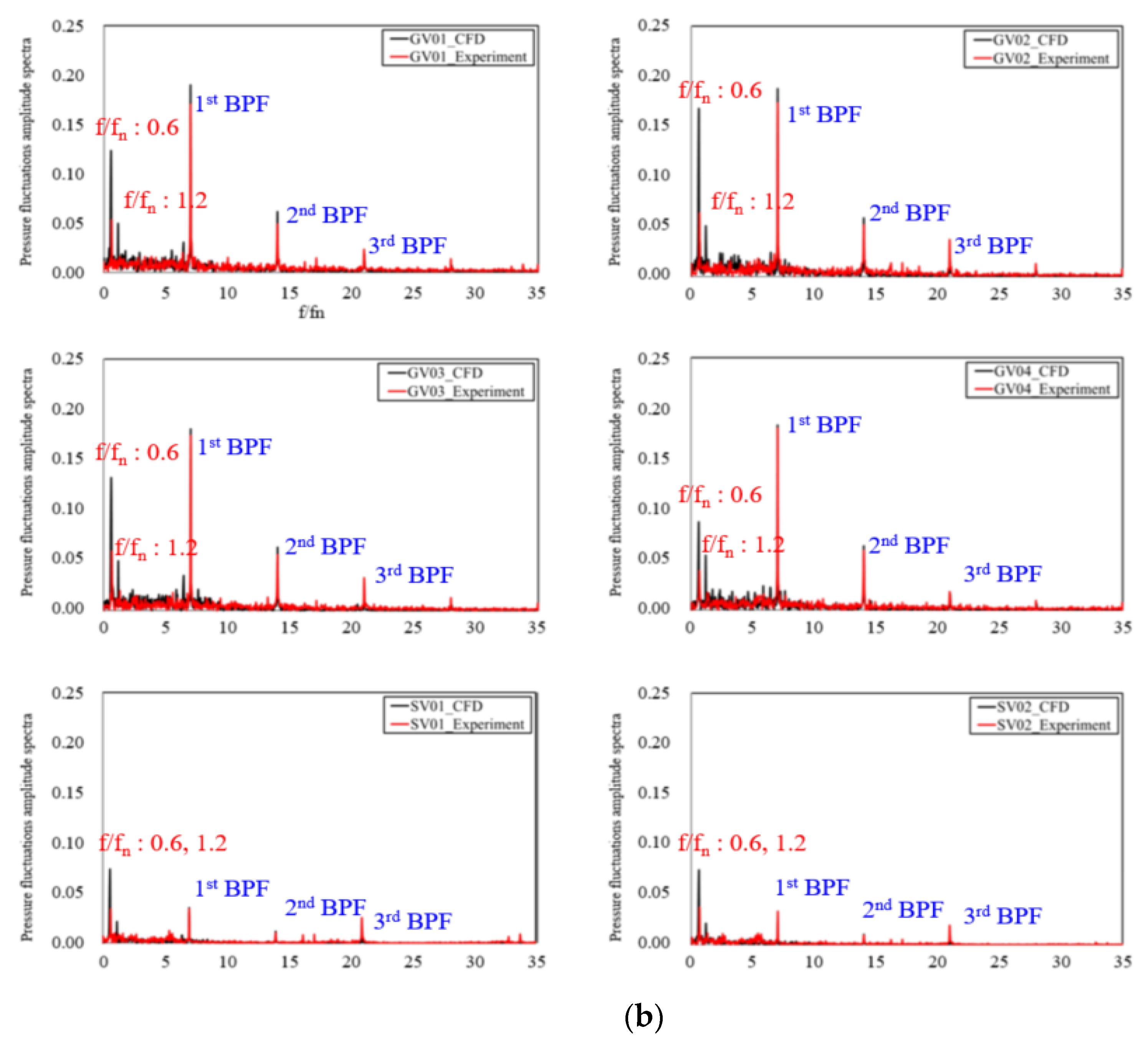
• The unsteady RANS equations in the SAS-SST model were discretized for a detailed analysis of the pressure characteristics. In the case of the full-scale model, there was no evidence of the RS. Therefore, the frequency spectra were only remarkable at f/f_n = 7.0, 14.0, and 21.0 (representing the first, second, and third BPF harmonics). In the case of the laboratory-scale model, the frequency spectra were remarkable at f/f_n = 0.6 (normalized frequency representing the RS) and at f/f_n = 7, 14, and 21 (first, second, and third BPFs). These results indicate an RS with a frequency propagation approximately 60% of the rotational speed of the runner.
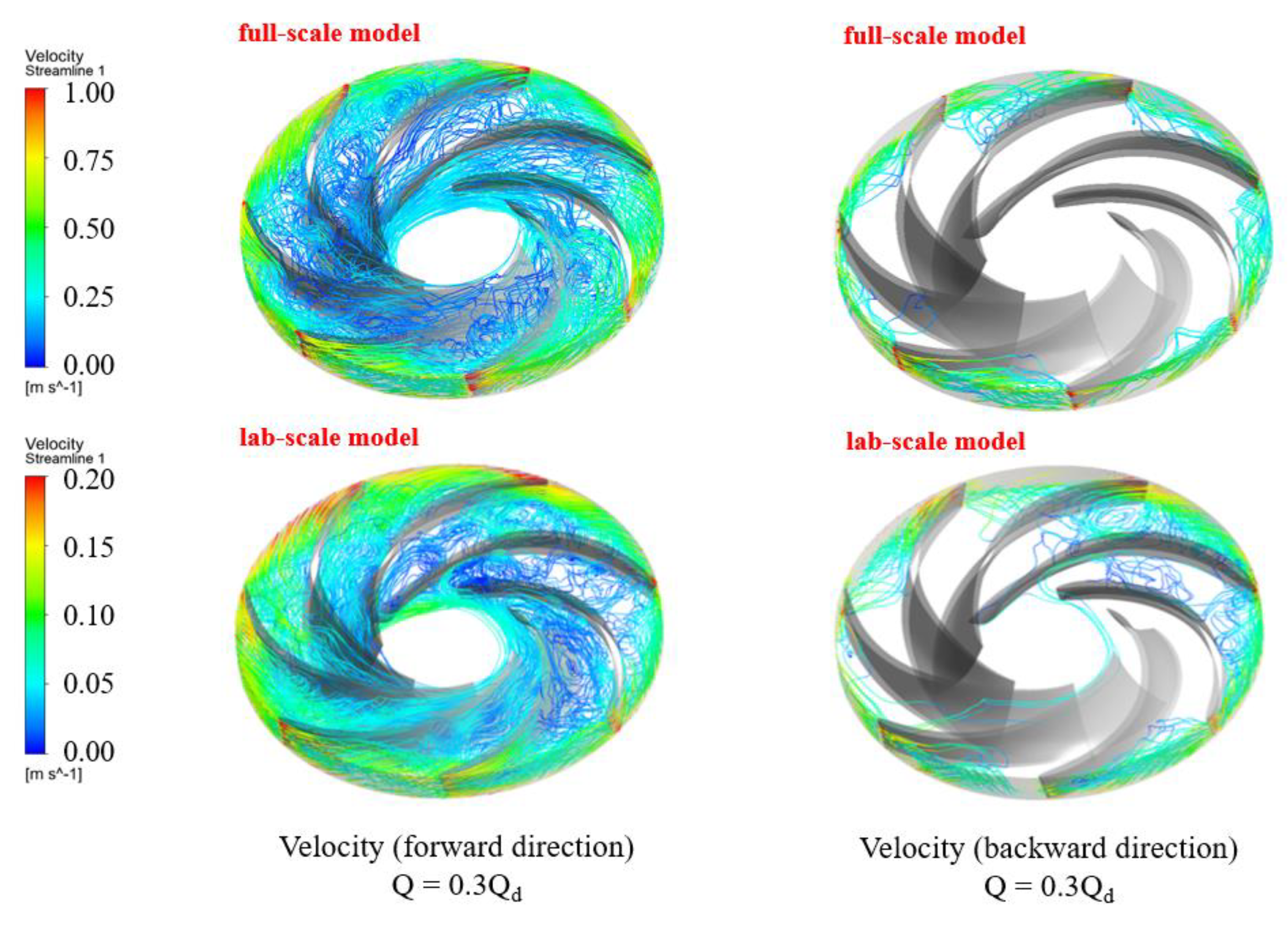
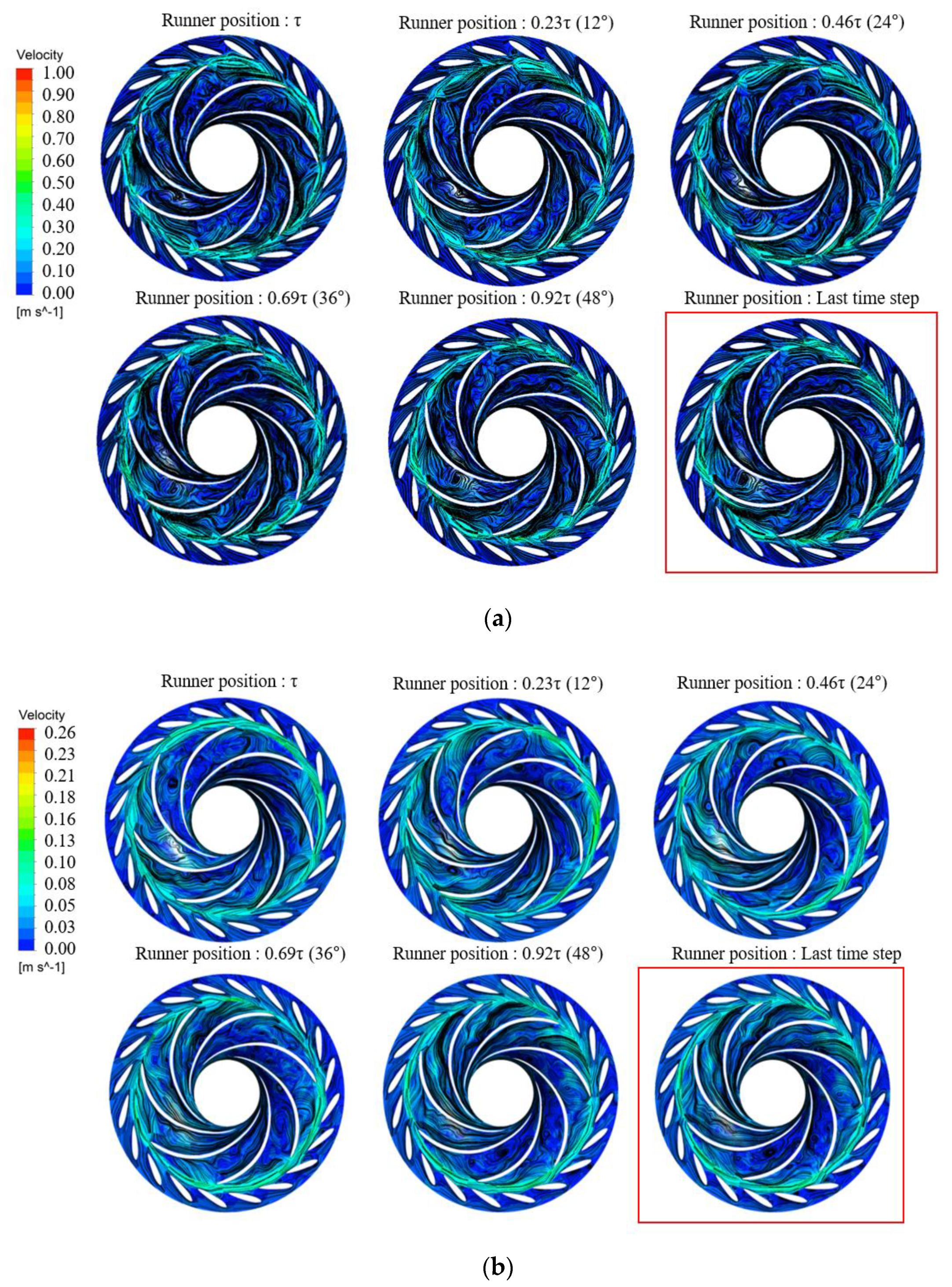
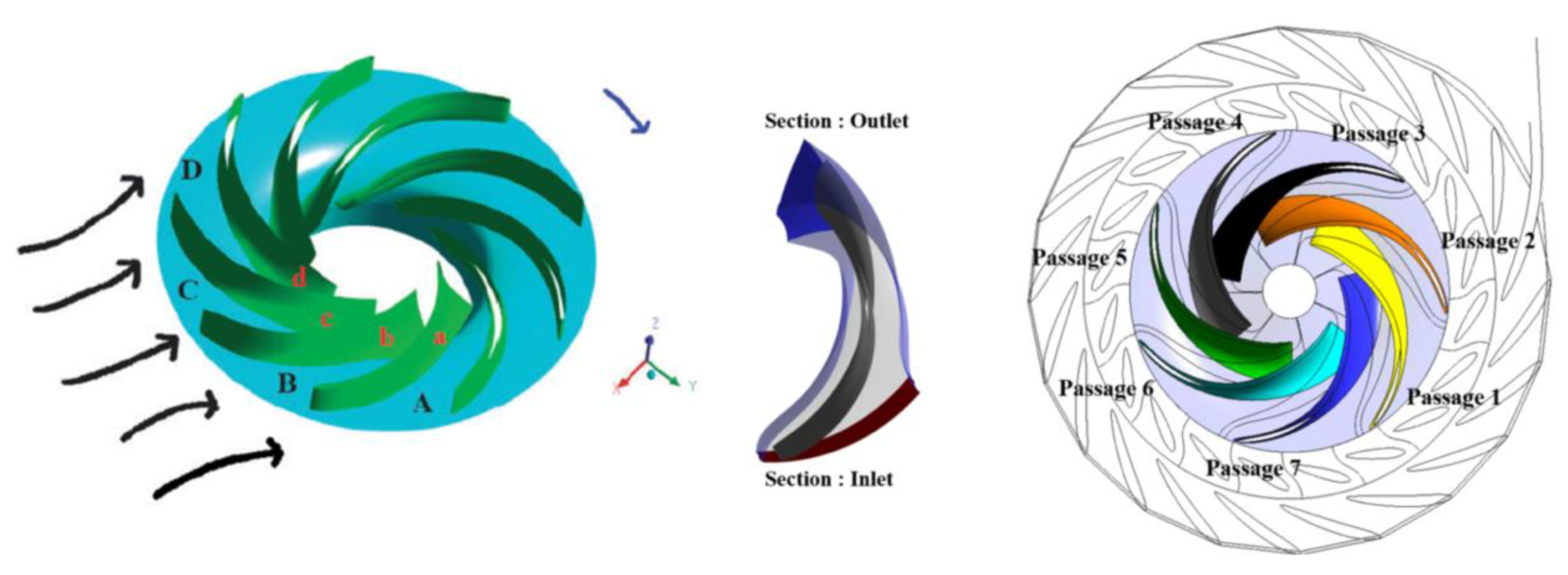
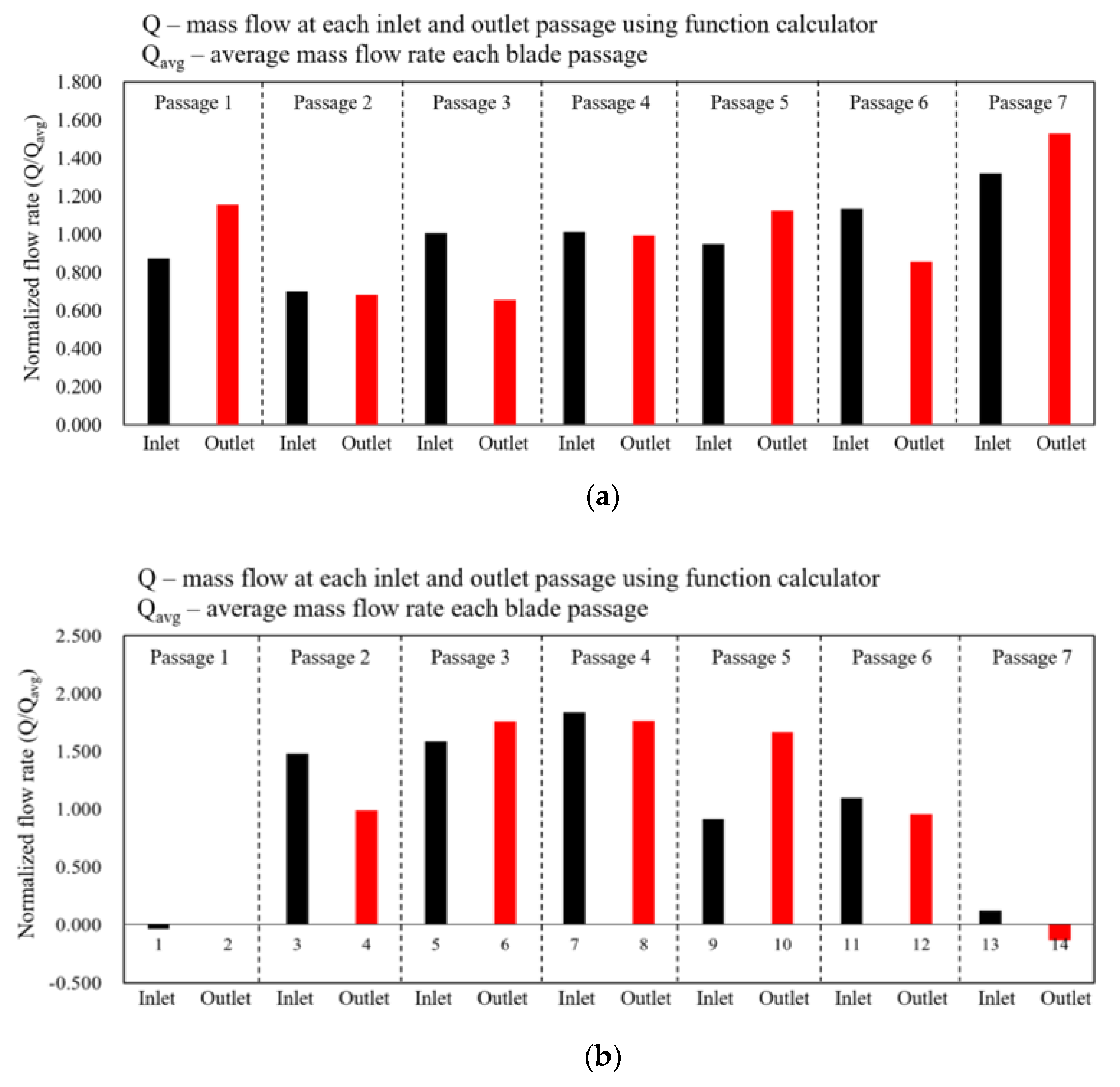
• The unsteady RANS equations in the SAS-SST model were discretized for a detailed analysis of the flow characteristics. Under the runaway condition of both models, the backflow became prominent. In the case of the full-scale model, the blade-loading distribution mostly showed a negative pattern. This means deflect flow from the flow blockage increasing the incidence angle whole the leading edge. As a result of checking the flow rate in and out of each flow passage, we found that there was no RS; therefore, the internal flow field was not completely blocked. In the case of the laboratory-scale model, some blade-loading distributions developed a positive shape, whereas others developed a negative shape. The characteristics of the passage adjacent to the stalled passage were also investigated.
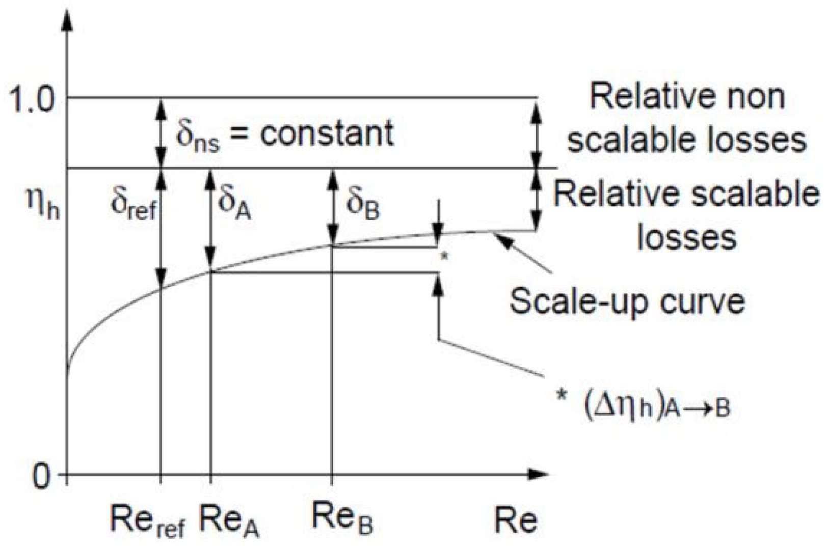
• The scale-up effect of the efficiency was calculated in hydraulically similar operating conditions having different Reynolds numbers. The numerical results obtained by calculating the hydraulic efficiency of the full- and laboratory-scale models were 95.15% and 91.38%, respectively. Based on the results of the scale-down model, the value calculated by predicting the hydraulic efficiency of the full-scale model by applying it to the formula was 94.61%. The scale-up effect between the models was found to be about 3.2%. The difference between the result calculated through numerical analysis and the value predicted through the calculation formula was 0.54%, confirming that the results obtained are fairly reliable.
• Predicting the efficiency and operating point of the scale effect through design is possible; however, slight variations occur in pressure and internal flow characteristics caused by hydrodynamic factors in the transition conditions. The reasons for these variations involve the composition of the grid system, turbulence model, surface roughness, and the development of an RS relative to the area of the flow passage, which require further investigation.

References

1. Lewi, N.S. Toward cost-effective solar energy use. Science 2017, 315, 798–801. [Google Scholar]
2. Herbert, G.J.; Iniyan, S.; Sreevalsan, E.; Rajapandian, S. A review of wind energy technologies. Renew. Sustain. Energy Rev. 2005, 11, 1117–1145. [Google Scholar] [CrossRef]
3. International Hydropower Association. Advancing Sustainable Hydropower, Activity and Strategy Report 2018–2019; International Hydropower Association: Paris, France, 2019. [Google Scholar]
4. Widmer, C.; Staubli, T.; Ledergerber, N. Unstable characteristics and rotating stall in turbine brake operation of pump-turbines. J. Fluids Eng. 2011, 133, 041101. [Google Scholar] [CrossRef]
5. Chen, W.M.; Kim, H.; Yamaguchi, H. Renewable energy in eastern Asia: Renewable energy policy review and comparative SWOT analysis for promoting renewable energy in Japan, South Korea, and Taiwan. Energy Policy 2014, 74, 319–329. [Google Scholar] [CrossRef]
6. Hemmati, R.; Saboori, H. Emergence of hybrid energy storage systems in renewable energy and transport applications–A review. Renew. Sustain. Energy Rev. 2016, 65, 11–23. [Google Scholar] [CrossRef]
7. International Electrotechnical Commission. Hydraulic Turbines, Storage Pumps and Pump-Turbines e Model Acceptance Tests; Standard No, IEC 60193; International Electrotechnical Commission: Geneva, Switzerland, 1999. [Google Scholar]
8. Zeng, W.; Yang, J.; Guo, W. Runaway instability of pump-turbines in S-shaped regions considering water compressibility. J. Fluids Eng. 2015, 137, 051401. [Google Scholar] [CrossRef]
9. Martin, C.S. Stability of pump-turbines during transient operation. In Proceedings of the 5th Conference on Pressure Surges BHRA, Hannover, Germany, 22–24 September 1986. [Google Scholar]
10. Hasmatuchi, V.; Farhat, M.; Roth, S.; Botero, F.; Avellan, F. Experimental evidence of rotating stall in a pump-turbine at off-design conditions in generating mode. J. Fluids Eng. 2011, 133, 051104. [Google Scholar] [CrossRef]
11. Yin, J.L.; Wang, D.Z.; Wei, X.Z.; Wang, L.Q. Hydraulic improvement to eliminate S-shaped curve in pump turbine. J. Fluids Eng. 2013, 135, 071105. [Google Scholar] [CrossRef]
12. Zuo, Z.; Liu, S.; Sun, Y.; Wu, Y. Pressure fluctuations in the vaneless space of high-head pump-turbines—A review. Renew. Sustain. Energy Rev. 2015, 41, 965–974. [Google Scholar] [CrossRef]
13. Zuo, Z.; Fan, H.; Liu, S.; Wu, Y. S-shaped characteristics on the performance curves of pump-turbines in turbine mode–A review. Renew. Sustain. Energy Rev. 2016, 60, 836–851. [Google Scholar] [CrossRef]
14. Cavazzini, G.; Houdeline, J.B.; Pavesi, G.; Teller, O.; Ardizzon, G. Unstable behavior of pump-turbines and its effects on power regulation capacity of pumped-hydro energy storage plants. Renew. Sustain. Energy Rev. 2018, 94, 399–409. [Google Scholar] [CrossRef]
15. Favrel, A.; Junior, J.G.P.; Landry, C.; Alligne, S.; Andolfatto, L.; Nicolet, C.; Avellan, F. Prediction of hydro-acosutic resonances in hydropower plants by a new approach based on the concept of swirl number. J. Hydrualic Res. 2019, 58, 87–104. [Google Scholar] [CrossRef]
16. Valentin, D.; Presas, A.; Valero, C.; Egusquiza, M.; Egusquiza, E.; Gomes, J.; Avellan, F. Transposition of the mechanical behaviour from model to prototype of Francis turbine. Renew. Energy 2020, 152, 1011–1023. [Google Scholar] [CrossRef]
17. Yang, Z.; Liu, Z.; Cheng, Y.; Zhang, X.; Liu, K.; Xia, L. Differences of flow patterns and pressure pulsations in four prototype pump-turbines during runaway Transient processes. Energies 2020, 152, 5269. [Google Scholar] [CrossRef]
18. Chen, T.J.; Luo, X.Q.; Guo, P.C.; Wu, Y.L. 3-D Simulation of a prototype pump-turbine during starting period in turbine model. In IOP Conference Series: Materials Science and Engineering; IOPscience: Bristol, UK, 2013; Volume 52, p. 052028. [Google Scholar]
19. Liu, J.T.; Liu, S.H.; Sun, Y.K.; Wu, Y.L.; Wang, L.Q. Numerical study of vortex rope during load rejection of a prototype pump-turbine. In IOP Conference Series: Earth and Environmental Science; IOPscience: Bristol, UK, 2012; Volume 15, p. 032044. [Google Scholar]
20. Suh, J.W.; Kim, S.J.; Kim, J.H.; Yang, H.M.; Joo, W.G.; Hwang, T.G.; Lee, K.H.; Shrestha, U.; Chen, Z.; Cho, H.K.; et al. Establishment of Numerical analysis method of Pump-turbine for Pumped Storage. KSFM J. Fluid Mach. 2019, 22, 22–29. [Google Scholar] [CrossRef]
21. Suh, J.W.; Kim, S.J.; Kim, J.H.; Joo, W.G.; Park, J.; Choi, Y.S. Effect of interface condition on the hydraulic characteristics of a pump-turbine at various guide vane opening conditions in pump mode. Renew. Energy 2020, 154, 986–1004. [Google Scholar] [CrossRef]
22. Spalart, P.; Allmaras, S. A one-equation turbulence model for aerodynamic flows. In 30th Aerospace Sciences Meeting and Exhibit; National Aeronautics and Space Administration: Washington, DC, USA, 1992; p. 439. [Google Scholar]
23. Jones, W.P.; Launder, B.E. The prediction of laminarization with a two-equation model of turbulence. Int. J. Heat Mass Transf. 1972, 15, 301–314. [Google Scholar] [CrossRef]
24. Mohammadi, B.; Pironneau, O. Analysis of the K-Epsilon Turbulence Model; IAEA: Vienna, Austria, 1993. [Google Scholar]
25. Chen, Y.S.; Kim, S.W. Computation of Turbulent Flows Using an Extended K-Epsilon Turbulence Closure Model; National Aeronautics and Space Administration: Washington, DC, USA, 1987.
26. Rotta, J.C. Statistische theorie nichthomogener turbulenz. Z. Phys. 1951, 129, 547–572. [Google Scholar] [CrossRef]
27. Rotta, J.C. Über eine methode zur Berechnung turbulenter Scherströmungen. Aerodyn. Vers. Rep. 1968, 69, A14. [Google Scholar]
28. Menter, F.R.; Egorov, Y. The scale-adaptive simulation method for unsteady turbulent flow predictions. Part 1: Theory and model description. Flow Turbul. Combust. 2010, 85, 113–138. [Google Scholar] [CrossRef]
29. ANSYS CFX-19.2. ANSYS CFX-Solver Theory Guide; ANSYS Inc.: Canonsburg, PA, USA, 2019. [Google Scholar]
30. Lee, Y.G.; Yuk, J.H.; Kang, M.H. Flow analysis of fluid machinery using CFX pressure-based coupled and various turbulence model. KSFM J. Fluid Mach. 2004, 7, 82–90. [Google Scholar] [CrossRef]
31. Zhang, Y.; Zhang, Y.; Wu, Y. A review of rotating stall in reversible pump turbine. Proc. Inst. Mech. Eng. Part C J. Mech. Eng. Sci. 2017, 231, 1181–1204. [Google Scholar] [CrossRef] [Green Version]
32. International Electrotechnical Commission. Field Acceptance Tests to Determine the Hydraulic Performance of Hydraulic Turbines, Storage Pumps and Pump-Turbines; Standard No, IEC 60041; International Electrotechnical Commission: Geneva, Switzerland, 1991. [Google Scholar]
33. OriginLab Corporation. Origin Pro 2019b, Origin Manual; OriginLab Corporation: Northampton, MA, USA, 2019. [Google Scholar]
34. National Instruments Corporation. LabVIEW, LabVIEW User; National Instruments Corporation: Austin, TX, USA, 2000. [Google Scholar]
35. Cavazzini, G.; Covi, A.; Pavesi, G.; Ardizzon, G. Analysis of the unstable behavior of a pump-turbine in turbine mode: Fluid-dynamical and spectral characterization of the S-shape characteristic. J. Fluids Eng. 2016, 138, 021105. [Google Scholar] [CrossRef]
36. Brennen, C.E. Hydrodynamics of Pumps; Cambridge University Press: Cambridge, UK, 1994; pp. 146–148. [Google Scholar]
Figure 1. Establishment of the numerical analysis procedure.
Energies 14 00525 g001
Figure 2. Procedure for analyzing the performance characteristics of model scales.
Energies 14 00525 g002
Figure 3. Geometrical structure and computational domain. (a) Hybrid (unstructured and structured) grid system. (b) Boundary conditions in turbine and pump modes.
Energies 14 00525 g003aEnergies 14 00525 g003b
Figure 4. Monitoring points in the computational domain and experimental setup: Positions of monitoring points in the (a) computational domain and (b) experimental setup.
Energies 14 00525 g004aEnergies 14 00525 g004b
Figure 5. Test facilities for performance evaluation: (a) Schematic of the experimental apparatus; (b) manufactured main components; (c) measurement of pressure pulsation setup and data extraction.
Energies 14 00525 g005aEnergies 14 00525 g005b
Figure 6. Comparison of performance characteristics between numerical simulations and experimental data in the full-scale model: (a) Turbine mode [20]; (b) pump mode [21].
Energies 14 00525 g006
Figure 7. Comparison of performance characteristics between numerical simulations (filled symbols) and experimental data (open symbols) in the laboratory-scale model.
Energies 14 00525 g007
Figure 8. S-shaped characteristics of model scales at 21.5° GVO: (a) Speed factor vs. discharge factor; (b) speed factor vs. torque factor.
Energies 14 00525 g008
Figure 9. S-shaped characteristics of model scales at 21.5° GVO: (a) Speed factor vs. discharge factor; (b) speed factor vs. torque factor.
Energies 14 00525 g009aEnergies 14 00525 g009b
Figure 10. S-shaped characteristics of model scales at 21.5° GVO: (a) Speed factor vs. discharge factor; (b) speed factor vs. torque factor.
Energies 14 00525 g010
Figure 11. Time histories of pressure fluctuations at representative monitoring points in the vaneless space under the runaway condition: (a) Full-scale model (ned: 2.1171, Qed: 0.0708 and Ted: 0.0052); (b) laboratory-scale model (ned: 1.9811, Qed: 0.0644 and Ted: 0.0033).
Energies 14 00525 g011aEnergies 14 00525 g011b
Figure 12. Time histories of pressure fluctuations at all monitoring points in the vaneless space under the normal and transition regions.
Energies 14 00525 g012
Figure 13. Time histories of low-pass-filtered signals at all monitoring points in the vaneless space under the runaway condition.
Energies 14 00525 g013
Figure 14. Frequency spectra of the pressure fluctuations under the runaway condition (obtained by the fast Fourier transform): (a) Full-scale model; (b) laboratory-scale model.
Energies 14 00525 g014aEnergies 14 00525 g014b
Figure 15. Comparison of the instantaneous radial velocity contours and vectors in the vaneless space between the models.
Energies 14 00525 g015
Figure 16. Comparison of the instantaneous velocity streamlines with forward and backward directions in the runner between the models.
Energies 14 00525 g016
Figure 17. Time history and representative velocity streamlines and contours on the runner mid-span section: (a) Full-scale model; (b) laboratory-scale model.
Energies 14 00525 g017
Figure 18. Schematic of the mechanism of the rotating stall (RS), and inlet and outlet section of a blade, and numbering of the passages.
Energies 14 00525 g018
Figure 19. Comparison of the blade-loading distribution under the runaway condition: (a) Full-scale model (blade 1–7); (b) laboratory-scale model (blade 1–7).
Energies 14 00525 g019
Figure 20. Normalized flow rate of runner channels under the runaway condition: (a) Full-scale model (blade 1–7); (b) laboratory-scale model (blade 1–7).
Energies 14 00525 g020
Figure 21. Efficiency change in hydraulically similar operating conditions having different Reynolds values (A and B).
Energies 14 00525 g021