Article

Creating a Virtual Test Bed Using a Dynamic Engine Model with Integrated Controls to Support in-the-Loop Hardware and Software Optimization and Calibration

by
Mohsen Mirzaeian
1,* and
Simon Langridge
2
1
FPT Industrial S.p.A., Via Puglia 15, 10156 Turin, Italy
2
FPT Motorenforschung AG, Schlossgasse 2, 9320 Arbon, Switzerland
*
Author to whom correspondence should be addressed.
Energies 2021, 14(3), 652; https://doi.org/10.3390/en14030652
Submission received: 15 December 2020 / Revised: 19 January 2021 / Accepted: 22 January 2021 / Published: 28 January 2021
(This article belongs to the Special Issue Internal Combustion Engine Performance)

Abstract

:
In the current study, a 0D/1D engine model built in the commercial code GT-Suite was coupled with the Electronic Control Unit (ECU) model created in the Simulink environment, aiming to more accurately predict the interaction of the engine and aftertreatment system (ATS) operating parameters, both during steady-state and transient maneuvers. After a detailed validation based on extensive experimental data from a heavy-duty commercial diesel Internal Combustion Engine (ICE), the engine model was fine-tuned and the 0D predictive diesel combustion model, DIPulse, was calibrated to best predict the combustion process, including engine-out NOx emissions. For correct prediction of the engine’s behavior in transient operations, the complete control strategy of the air path, including boost, exhaust gas recirculation (EGR), main and pilot Start of Injection (SOI), injection pressure, and exhaust flap, was implemented in the Simulink environment. To demonstrate the predictive capability of the model, a hot World Harmonized Transient Cycle (WHTC) was simulated, obtaining good agreement with the experimental data both in terms of emissions and performance parameters, confirming the reliability of the proposed approach. Finally, a case study on possible fuel consumption improvement through thermal insulation of the exhaust manifold, exhaust ports, and turbocharger was carried out.

1. Introduction

The need to reduce man-made greenhouse gas emissions has led to new and challenging targets for future CO2 emissions [1]. The European Union (EU) Commission proposes a reduction of the average CO2 emissions of new heavy-duty vehicles by 15% and 30% in 2025 and 2030, respectively, compared with the 2019 baseline.
Moreover, EU regulation limits for emissions are becoming more strict, and type-approval procedures will also change radically with the introduction of World Harmonized Transient Cycle (WHTC) and Real Driving Emission (RDE) tests. The main challenge in the automotive industry is to find an optimal balance between fuel consumption and drivability within the boundaries set by emissions legislation, prompting Original Equipment Manufacturers (OEMs) to utilize different technologies such as exhaust gas recirculation (EGR) [2], Variable Valve Actuation (VVA) [3,4], exhaust line and turbocharger insulation [5], cylinder deactivation [6], and high-injection pressure systems [7] on the engine side together with complex aftertreatment layouts [8] with catalytic heating [9].
Since new complex engine and aftertreatment systems demonstrate considerable interactions and interdependencies [10], stand-alone aftertreatment system considerations might not lead to the optimal solution for the whole system. As total system complexity increases, using robust and reliable engine simulation models will bring aftertreatment system (ATS) boundary conditions into the loop during ATS development. The co-simulation activity presented here is the first step to a dedicated full-system simulation tool that will eventually evaluate the cost and benefit interactions of all the technologies described above.
Detailed simulation of charge motion, in-cylinder flow, and combustion [11,12,13] are usually carried out using 3D Computational Fluid Dynamics (CFD) codes. However, the relatively high computational costs of these methods have restricted their application to some extent, particularly when considering complex systems. In this context, 0/1D models, which are traditionally less computationally intensive, can be used as reliable simulation tools.
Different types of 0/1D diesel combustion models have been proposed in the literature [14,15]. In this study, the commercially available predictive combustion model DIPulse [16,17], developed by Gamma Technologies (Westmont, United States), was used to accurately predict fuel burn rate and engine performance parameters. Moreover, engine-out NOx emissions were predicted by the extended Zeldovich method [18].
Diesel engine system controls [19] are another important consideration for modern engines to further improve fuel consumption and reduce NOx and particulate matter; modeling of real control strategies for air and injection systems is necessary to reliably predict engine behavior, especially under transient conditions.
In order to create a virtual test bed, a physical engine model should be coupled with the correct control strategy. Martin et al. [20] created a virtual test bed using a gas dynamics software called VEMOD. A virtual Electronic Control Unit (ECU) model was used in this study, which might control the engine differently from the real ECU model, especially under transient conditions. For instance, the Proportional, Integral, and Derivative (PID) parameters (Proportional, Integral, and Derivative gains), transient correction at the start of injection, transient correction of injection pressure, and flap actuation during transient engine operations will affect the results both in terms of performance and emissions.
In this study, the complete airpath model of the ECU was developed in the Simulink environment to control the engine model and, together with the detailed combustion and emissions models, engine performance parameters both during steady state and, more importantly, during transient operation were predicted accurately.
The airpath control part of the real ECU model offers the possibility to run the engine with the real control strategy in the Software-in-the-Loop (SiL) ambient, replicating exactly the engine control behavior in real transient driving conditions. In previous studies [20], more simplified approaches have been suggested.
The model is further utilized to simulate a hot WHTC and compare the measurements. One of the most important parameters for ATS performance is the temperature after the turbine, and, as will be shown in the results (Section 4.3), using the ECU control strategy and suggested combustion model, temperature prediction was improved compared with prior research such as the paper published by J. Martin et al. [20], which shows more than a 100 °C error in turbine outlet temperature. The error rate is reduced to 30 °C in the current study, which resulted in more precise prediction of ATS performance. Finally, after validation of the model, the benefits of thermal insulation of the exhaust manifold, exhaust ports, and turbocharger on fuel consumption were evaluated. This case study indicates how a reliable and computationally efficient 0D/1D simulation model can be used to not only decrease the test bench activity and chassis dyno experimental campaign, but also to better target any testing activity, once at the test bench. Furthermore, considering that GT-Suite is utilized extensively in the Internal Combustion Engine (ICE) analysis, the current study shows the capability to create a virtual test bed using GT-Suite coupled with ECU control models.

2. Engine Characteristics and Operating Points

The engine used for the study is a heavy-duty six-cylinder diesel engine, equipped with a common rail, high-pressure EGR system, and Variable Geometry Turbocharger (VGT), the main characteristics of which are described in Table 1.
The experimental tests were performed over a complete engine operating map with the speed varying from 550 to 2200 rpm, as shown in Figure 1.

3. Simulation Model Description

The simulation activity begins with the careful validation of the detailed model. As shown in Figure 2, the detailed model is divided into three main parts, namely: engine, turbocharger, and aftertreatment. The engine model was created by reducing the 3D model of the engine airpath to 1D, and by converting it into simple flowsplits and pipes using the GTSuite tool GEM3D.
The turbocharger is traditionally modeled using maps of flow characteristics provided by the supplier. Particularly for turbine maps, heat transfer is most often neglected. This does not significantly affect general engine performance, but does affect temperature prediction at the turbine outlet and, thus, aftertreatment inlet temperature [21,22,23,24]. Therefore, we decided to include a sub-model that takes thermal effects into account. The heat transfer path from turbocharger to coolant and environment is shown in Figure 3. The nodal model of heat transfer in the turbocharger utilized in this work was proposed by Serrano et al. [25,26,27].
As shown in Figure 4, three thermal masses are considered in order to account for the shaft/bearings, turbine, and compressor wheels. The turbine and compressor volutes are simplified [28,29] to a pipe (Figure 5) with the diameter and length calculated by Equations (1) and (2). Due to a lack of experimental data regarding heat transfer in turbochargers, the limits and procedure recommended in [16] were used.
l v o l = l l + r 1 + r 2 2 π
d v o l = 4 V vol π l v o l
In 0D simulations, the aftertreatment line (Figure 6) is usually modeled by the calibration of a series of reactions in order to predict tailpipe emissions. In this case, since the thermal behavior and pressure drop of the ATS are of interest, and not the tailpipe NOx, and to improve the simulation time, the aftertreatment is modeled considering the actual thermal inertia of the system, such as the material properties and size of each component, without solving any reactions; hence, the heat generated or absorbed by the reactions is neglected. In a further activity, not presented here, the model was also coupled with a full chemical ATS 1D model.

3.1. Predictive Combustion Model

In order to take into account the effect of different EGR rates, Start of Injection (SOI), rail pressure, pilot injection, and operating conditions on combustion, the DIPulse predictive combustion model [16,17], was used. The DIPulse model separates the in-cylinder content into three thermodynamic zones, each with their own composition and temperature [16].
All trapped mass at intake valve closure is considered the main unburned zone. The spray is divided into two basic parts, namely unburned and burned zones. The former includes the fuel and entrained gas, and the latter contains the product of combustion. The model takes into account the fuel evaporation, mixing, and burning process [16]. The combustion sub-model contains four calibration multipliers:
  • Entrainment Rate (ERM);
  • Ignition Delay (IDM);
  • Premixed Combustion Rate (PCRM); and
  • Diffusion Combustion Rate (DCR).
A Design of Experiment (DoE) [30] technique, combined with a Genetic Algorithm (GA), was used to find the optimum calibration parameters with the aim of minimizing the Root Mean Squared (RMS) error between experimental and simulated burn rates. The calibration approach has been discussed in more detail in [17,31]. Optimized values of the calibration parameters are shown in Table 2.

3.2. Engine-Out NOx Model

The NOx calculation is based on the extended Zeldovich mechanism [18]. The reactions are shown in Equation (3).
{ O   +   N 2   =   N O   +   N   N 2   o x i d a t i o n   r a t e   e q u a t i o n   N   +   O 2   =   N O   +   O   N   o x i d a t i o n   r a t e   e q u a t i o n   N   +   O H   =   N O   +   H   O H   r e d u c t i o n   r a t e   e q u a t i o n  
Two calibration multipliers are used:
  • a multiplier for the predicted net rate of NOx formation; and
  • a multiplier for the activation energy of the N2 oxidation rate equation.
A DoE analysis was carried out with the aim of minimizing the error function that was defined based on the difference between the simulated and measured NOx engine-out concentration.

3.3. Airpath Control Model

The ECU airpath control model includes boost pressure, EGR, injection pressure, pilot and main SOI, and exhaust flap control. Depending on the engine and ATS conditions, the ECU combustion model can vary between different modes, including normal mode, cold start mode, and regeneration mode.
The engine model passes the physical operating parameters to the ECU model, and the control parameters then adjust to the requested engine operation. It is important to note that the details of the ECU model could not be published for confidentiality reasons (Figure 7).
The boost pressure is closed-loop and contains four main governors:
  • a boost pressure governor;
  • an exhaust pressure—steady governor;
  • an exhaust pressure—transient governor; and
  • a turbine speed governor.
Using the engine mode and physical parameters of the engine model, such as turbocharger speed, boost pressure, exhaust pressure, and the corresponding setpoints and gradients, a state machine decides which governor should be active. For instance, if the turbocharger speed exceeds its maximum limit, the turbocharger speed governor will activate to protect the turbocharger.
The EGR control is open-loop over the complete engine map. The desired EGR rate is a function of injected fuel, speed, and environmental conditions, which are part of the ECU model in the form of calibration maps. In order to correctly recirculate the desired EGR quantity, the EGR valve model calculates the desired valve opening position based on the engine mode and the following input signals:
  • desired mass flow through the EGR valve;
  • pressure before EGR valve;
  • pressure after EGR valve; and
  • temperature before EGR valve.
The SOI and injection pressure controllers are of the open-loop type. The SOI and injection pressure are calculated based on the maps which are the function of operating mode, EGR rate, injected fuel, and engine speed. The base value will be corrected under transient conditions.
The exhaust flap control is also of the open-loop type. The exhaust flap is inactive in the normal operation mode of the engine. The exhaust flap’s base position is calculated as a function of injected fuel and engine speed, which is further scaled based on the distance of the Selective Catalytic Reduction (SCR) temperature from a threshold level such that, as the difference between the SCR temperature and the threshold level reduces, the exhaust flap scaling acts to increase the flap opening.

3.4. ECU and GT-Suite Coupling

After the creation of the GT-Suite model, the ‘SimulinkHarness’ template should be included in the model. In this template, all input (from GT-Suite to Simulink) and output (from Simulink to GT-Suite) parameters should be defined and linked to the relevant part of the model. The input parameters required by the control strategy are the physical parameters, including engine speed, requested fuel, air flow rate, boost pressure, and turbocharger speed. The output parameters are the start of injection, injection pressure, VGT position, main and pilot injection, flap position, and EGR valve position.
In the next step, the GT-SUITE Model’s S-Function block should be inserted into the ECU model. This block can be found in the Simulink Library Browser. As can be observed in Figure 7, all input and output parameters are linked in the S-function GT-Suite block and the ECU model. Afterwards, within the GT-SUITE Model’s S-Function block, it is necessary to specify the number of inputs and outputs, the time step, and the GT-Suite model’s name.
For example, regarding the combustion control, the injection pressure, SOI, and injection quantities of all injection events are transferred from Simulink (the ECU model) to GT-Suite, where the DIPulse predictive combustion model will evaluate the burn rate and consequently the in-cylinder pressure.
Further information about the requirements for, and descriptions of, the GT-Suite and Simulink coupling can be found in [16].

4. Results and Discussion

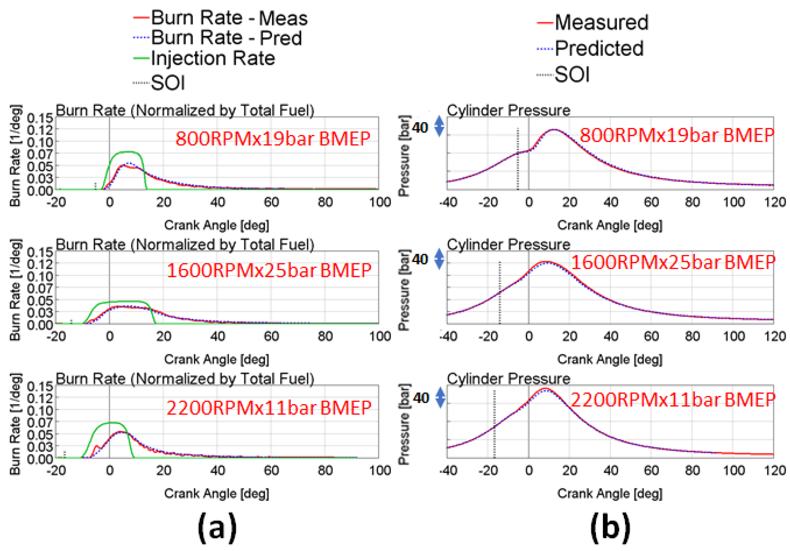
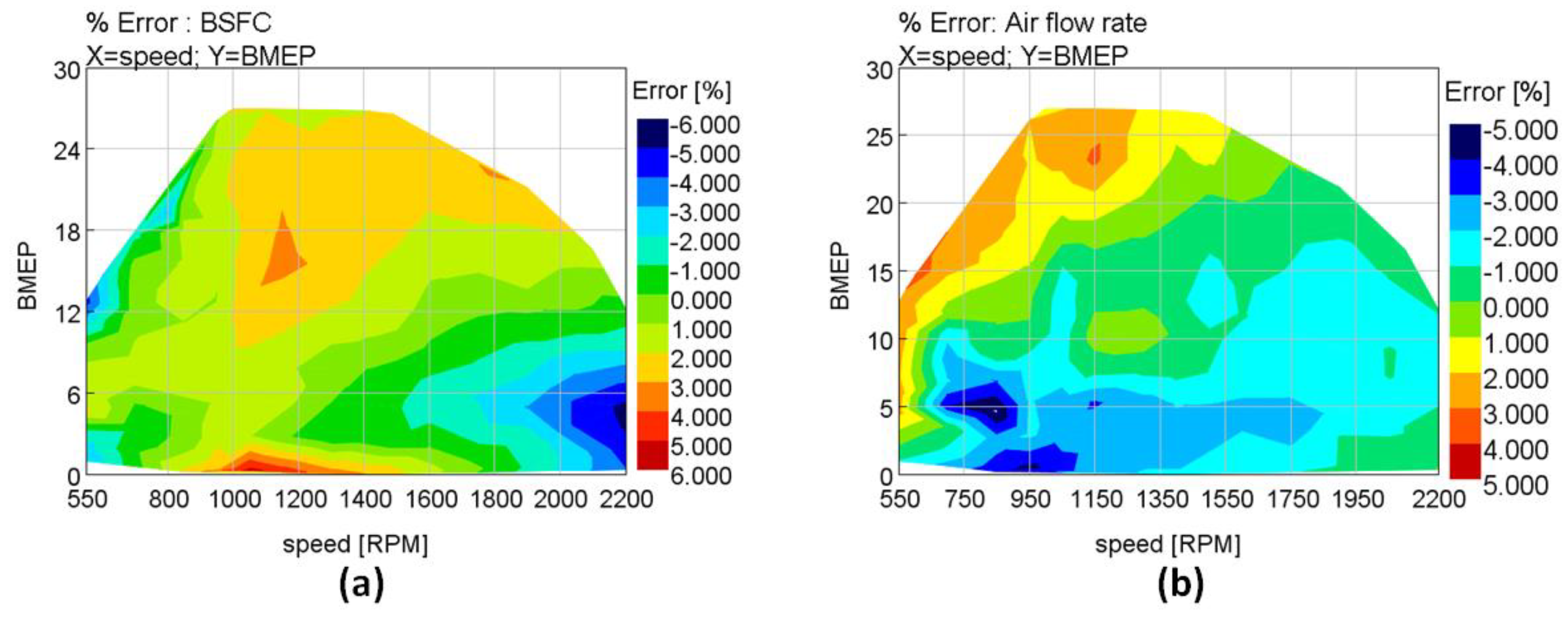
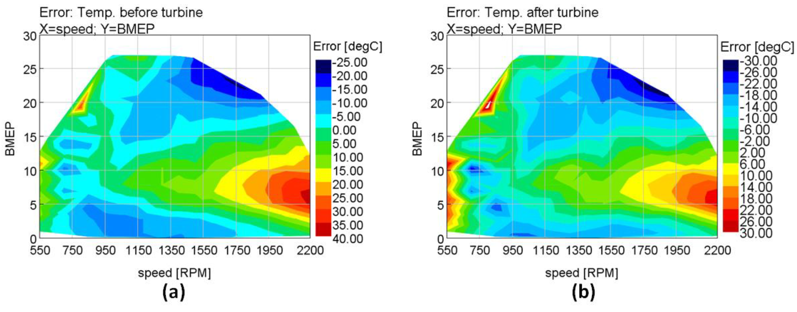
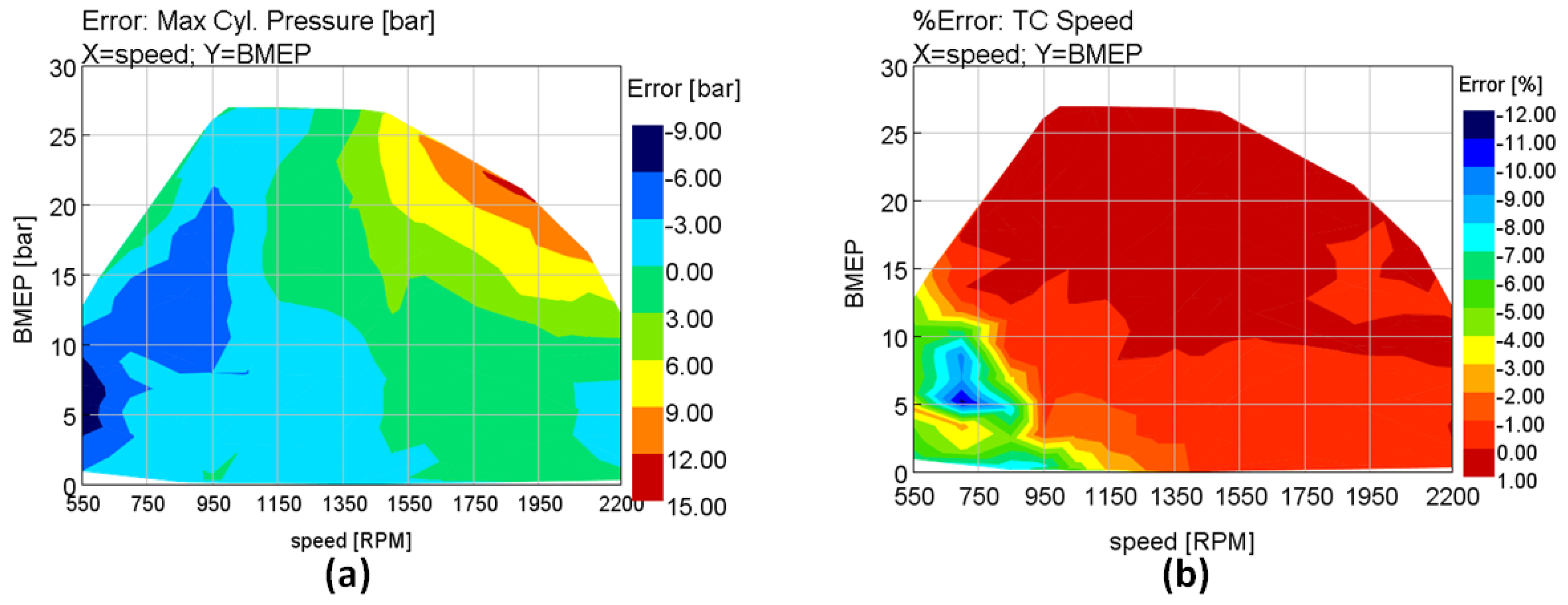
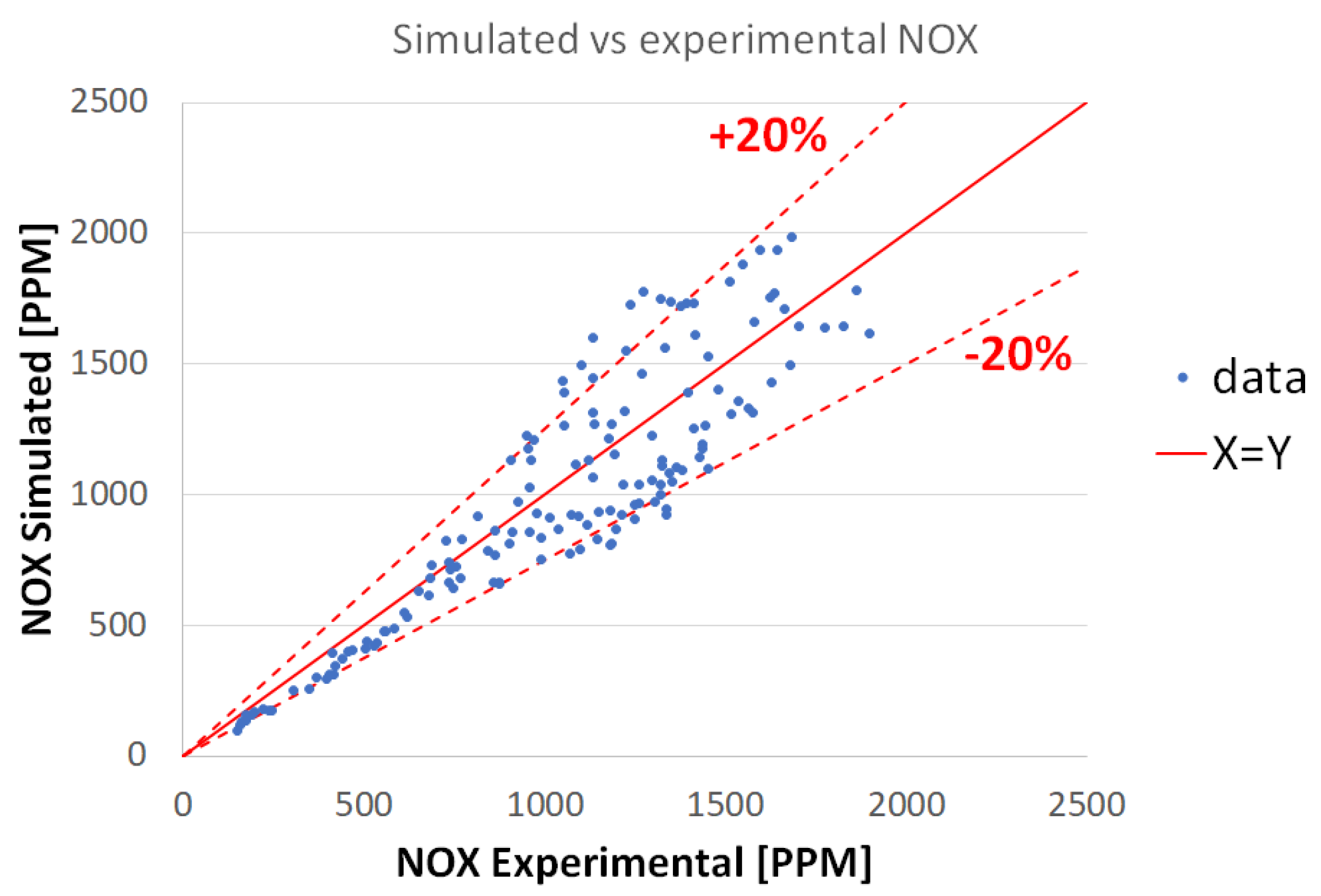
4.1. Steady State Simulation

After the DIPulse combustion model was calibrated as described in Section 3.1, the optimized DIPulse multipliers were fixed for all engine operating points, and the accuracy of the model was confirmed for all operating points on the map. The pressure and burn rate profiles are presented in Figure 8 for three speeds at full load. Good agreement was obtained between the predicted burn rates and the in-cylinder pressure with measured values. Similarly good agreement was achieved across the entire engine operating map.
To demonstrate the predictive capability of the model, the errors between experimental and simulated values of Brake Specific Fuel Consumption (BSFC) (Figure 9a), air mass flow rate (Figure 9b), temperature before turbine (Figure 10a), temperature after turbine (Figure 10b), peak cylinder pressure (Figure 11a), and turbocharger speed (Figure 11b) are shown as contour plots in the engine map. The absolute average errors are 1.77%, 1.46%, 9.3 °C, 10.8 °C, 2.9 bar, and 1.2%, respectively.
As shown in Figure 12, the simulated engine-out NOx values versus the measured values have an R-squared coefficient of 0.81 and an error band of 20% at most of the points on the engine map.

4.2. Transient Operation Simulation

The engine’s behavior was numerically and experimentally analyzed during transient operation. An abrupt change in pedal position (from 0 to 100%) was specified to occur at a constant engine speed. The objective was to define the response time of the turbocharger. The tests were carried out at two different speeds (900 rpm and 1900 rpm). The results are shown in Figure 13 and Figure 14.

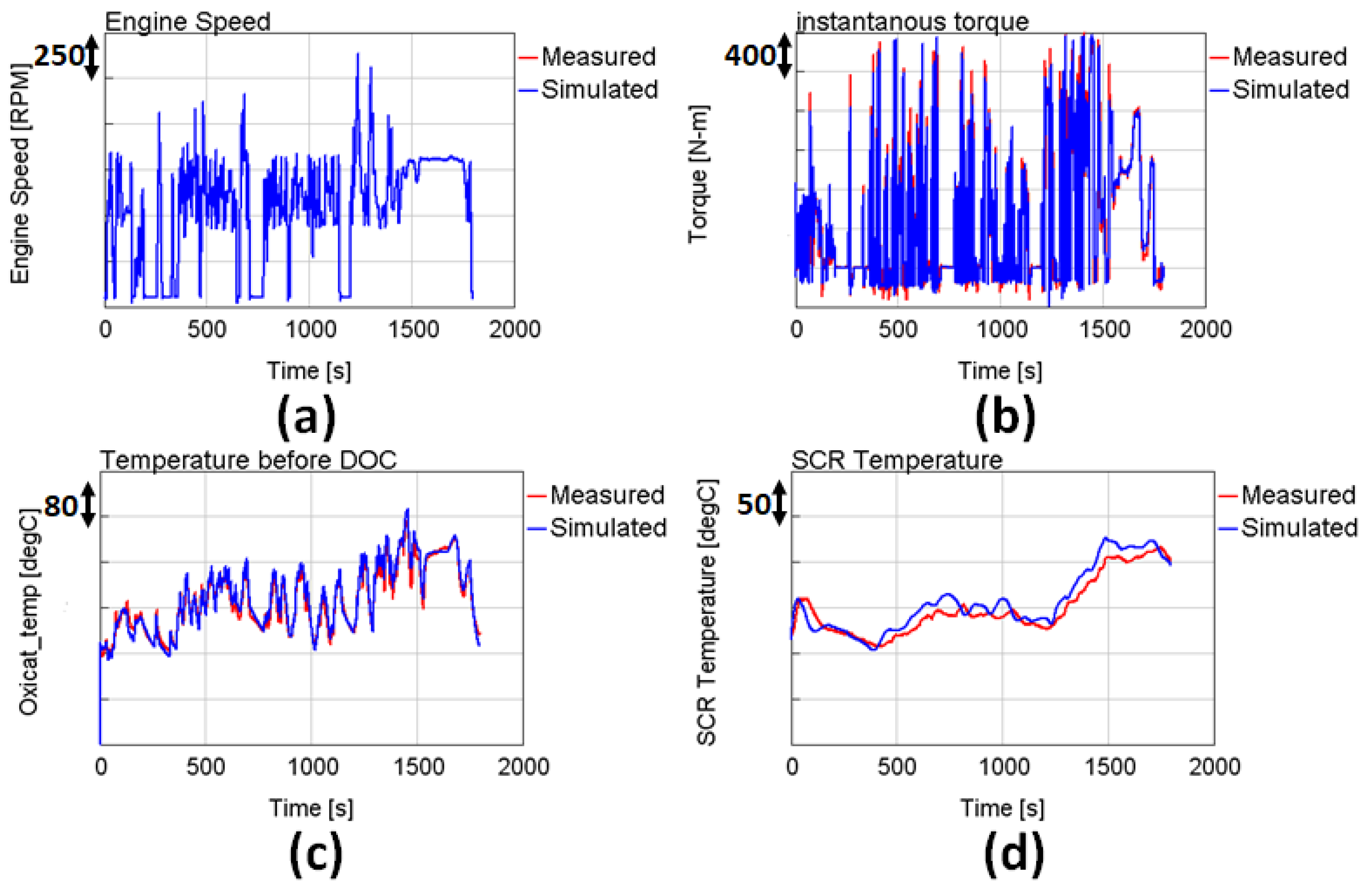
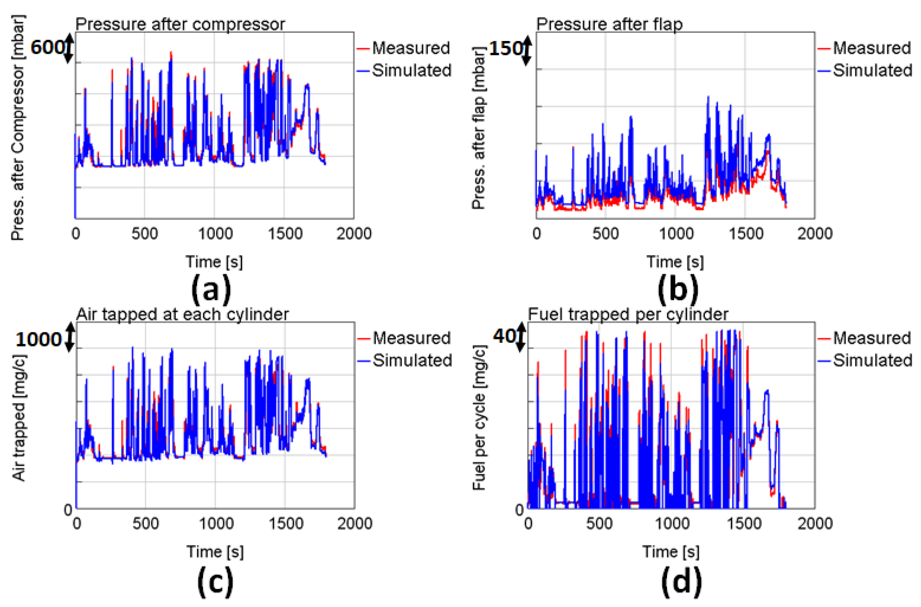
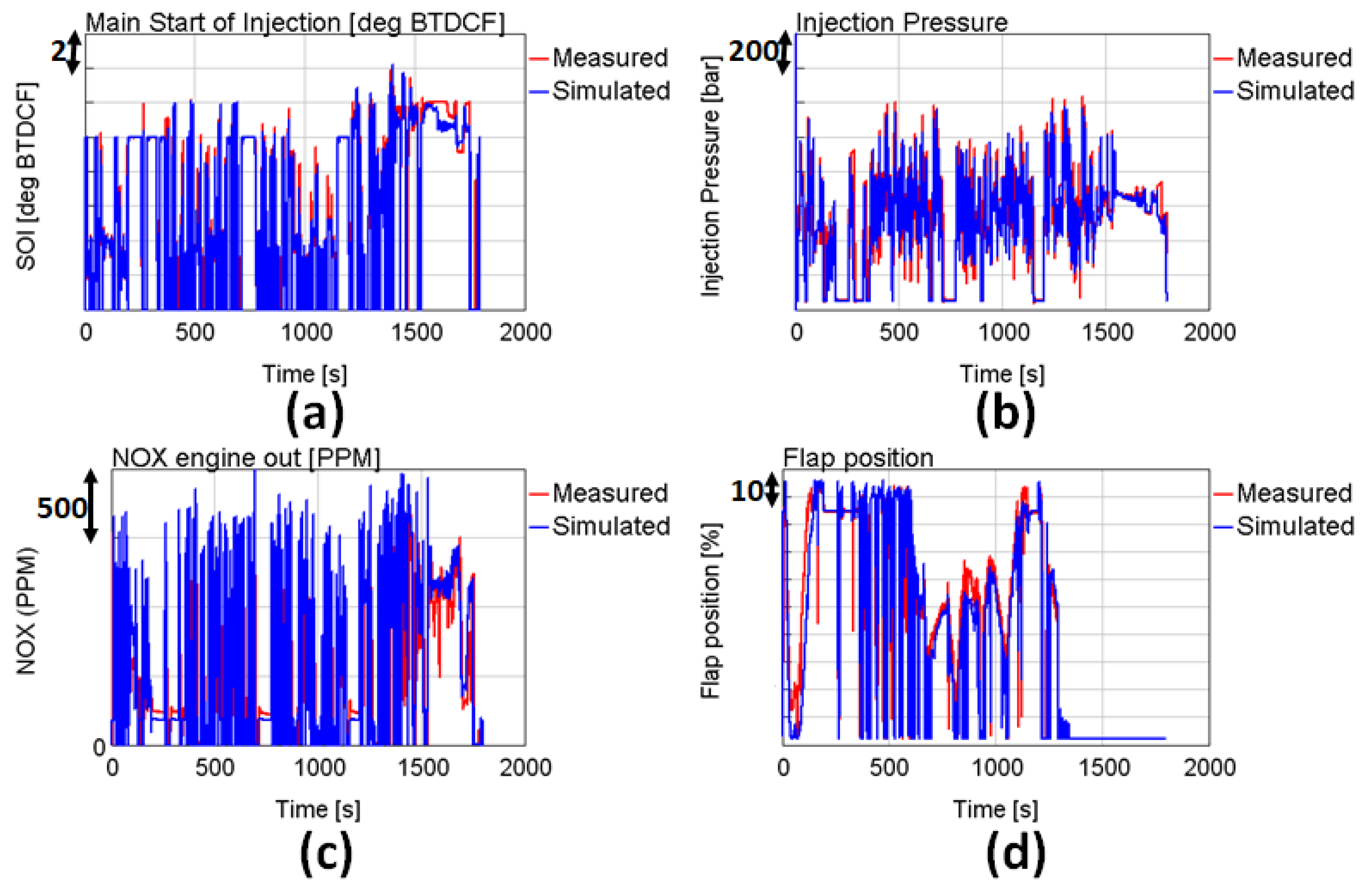
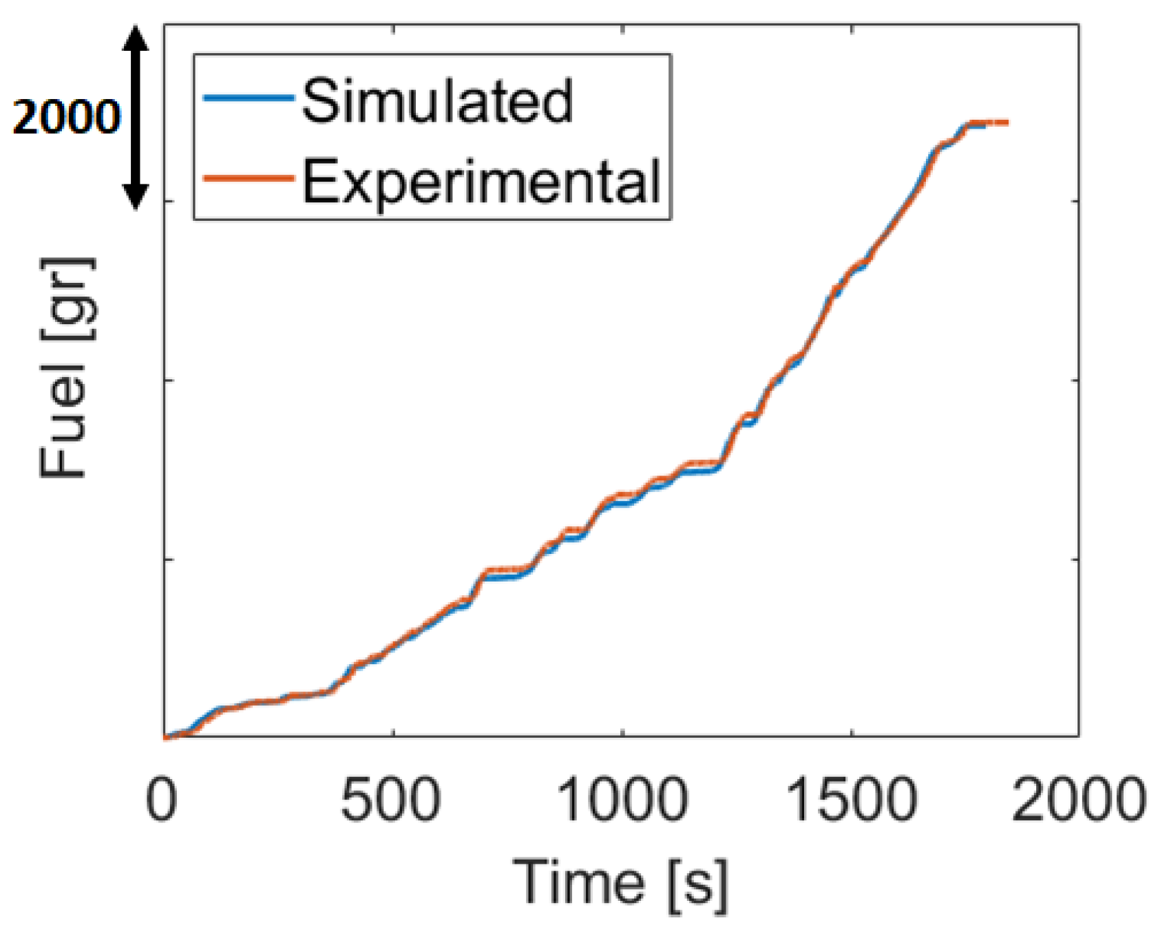
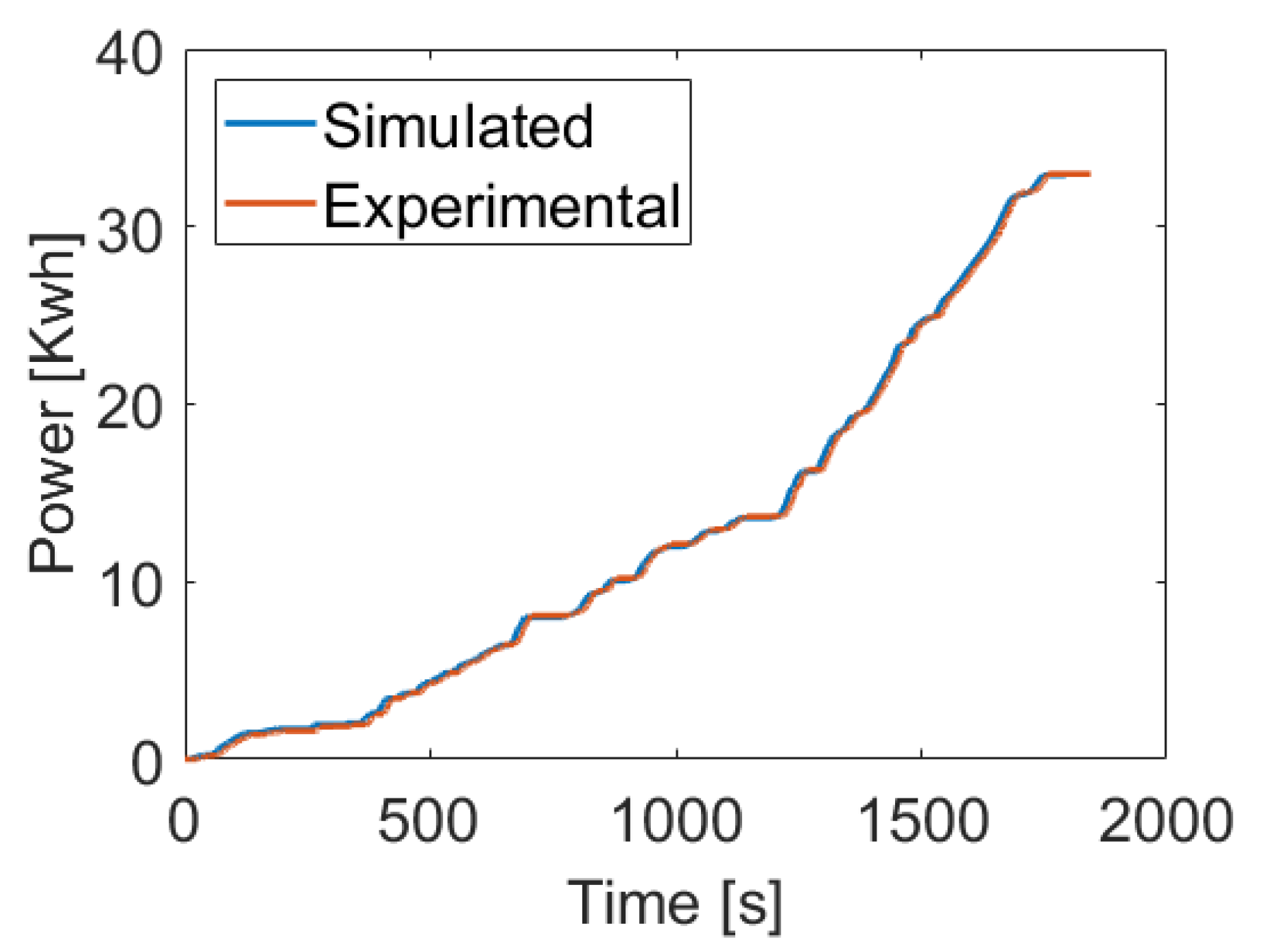
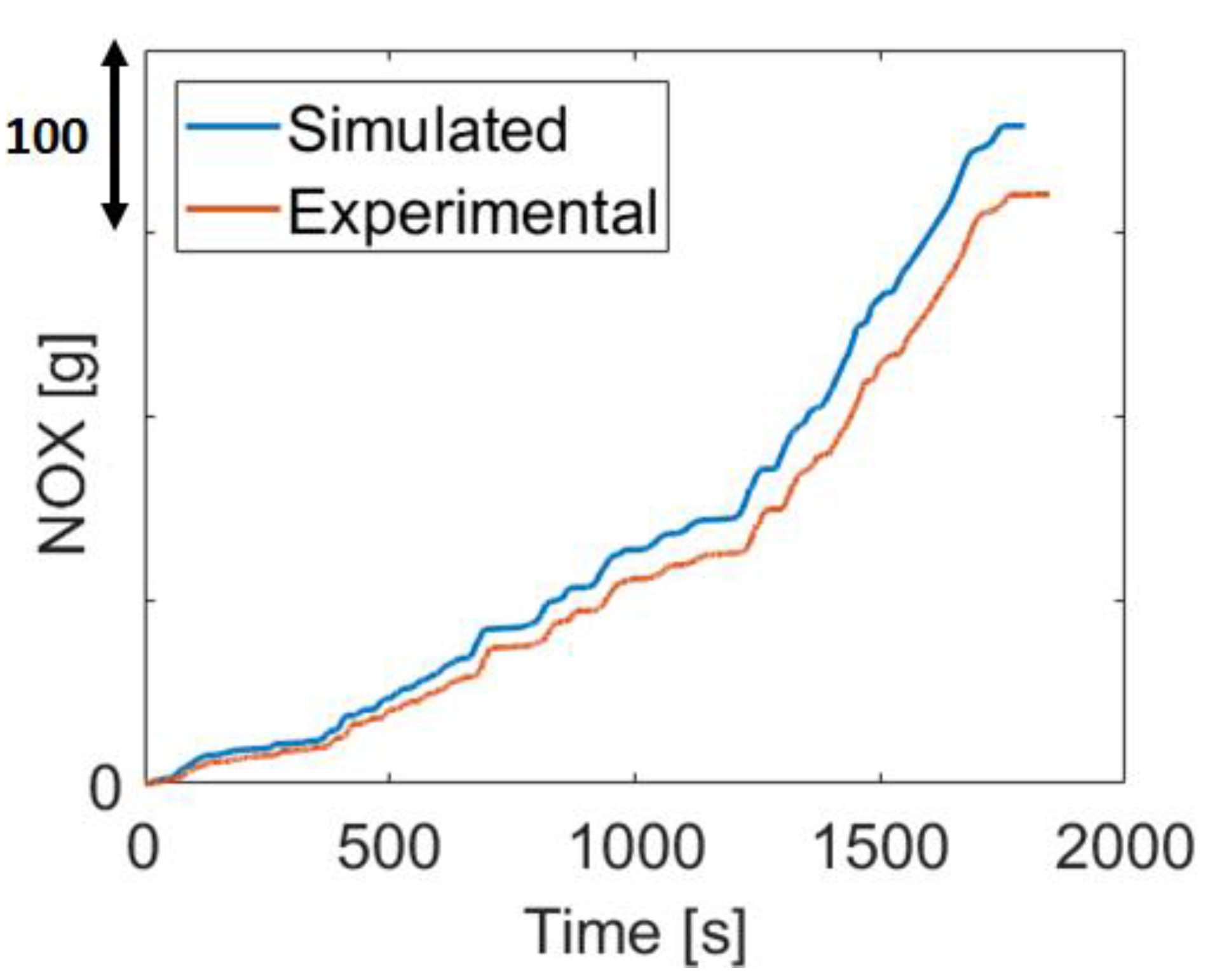
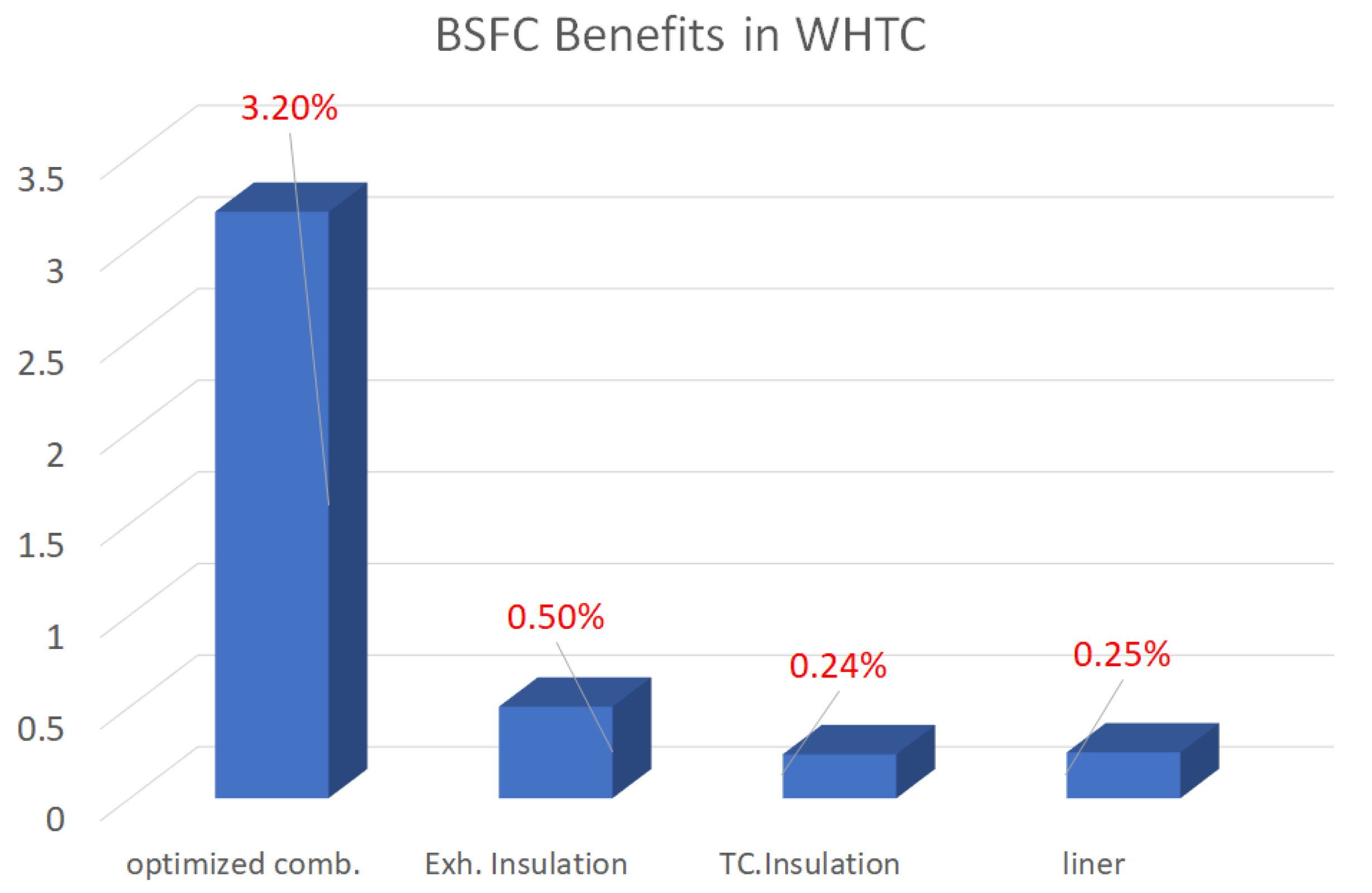
4.3. WHTC Simulation

We used the simulation to analyze the engine’s behavior during a hot World Harmonized Transient (WHT) homologation cycle with the aim of assessing the predictive capability of the model. The engine speed and torque traces (typical WHTCs) are the main inputs of the model. The engine speed was imposed, while the torque was controlled by the fueling within the limits defined in the ECU (smoke map and maximum fuel injection).
As shown in Figure 15, there is satisfactory agreement between the experimental and simulated temperature before diesel catalyst oxidation and SCR temperature. A comparison of the other operating parameters is shown in Figure 16.
The exhaust flap and combustion are controlled by the SCR temperature. Two combustion modes were used in the WHTC. In the first part (from 0 s to about 1350 s), the ‘late combustion’ mode was used, in which the exhaust flap was active (Figure 17d) since the SCR temperature was below the specified threshold temperature in the calibration (Figure 17b). In the second part (from 1350 s to 1800 s), the ‘normal combustion mode’ was active and the exhaust flap was fully open (Figure 17d). The difference in SOI between the two combustion modes is shown in Figure 18. It can be observed that the difference in SOI is larger at a low speed and in the low load region.
A comparison of the simulated and experimental cumulative injected fuel, power, and engine-out NOx emissions is shown in Figure 19, Figure 20 and Figure 21, respectively. The error in BSFC (g/kWh) and engine-out NOx (g/kWh) emissions is 0.3% and 11.5%, respectively, over the entire cycle.

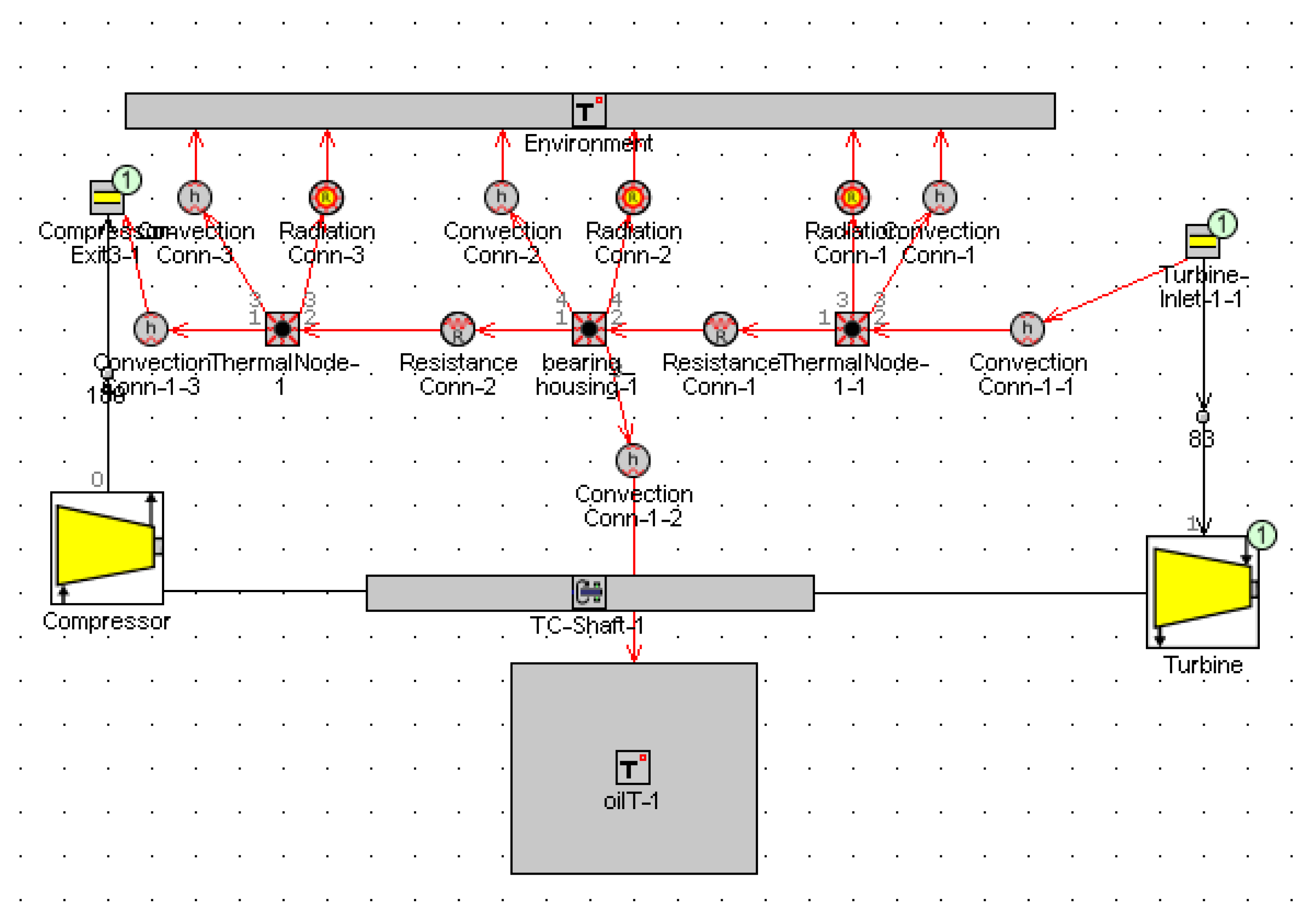
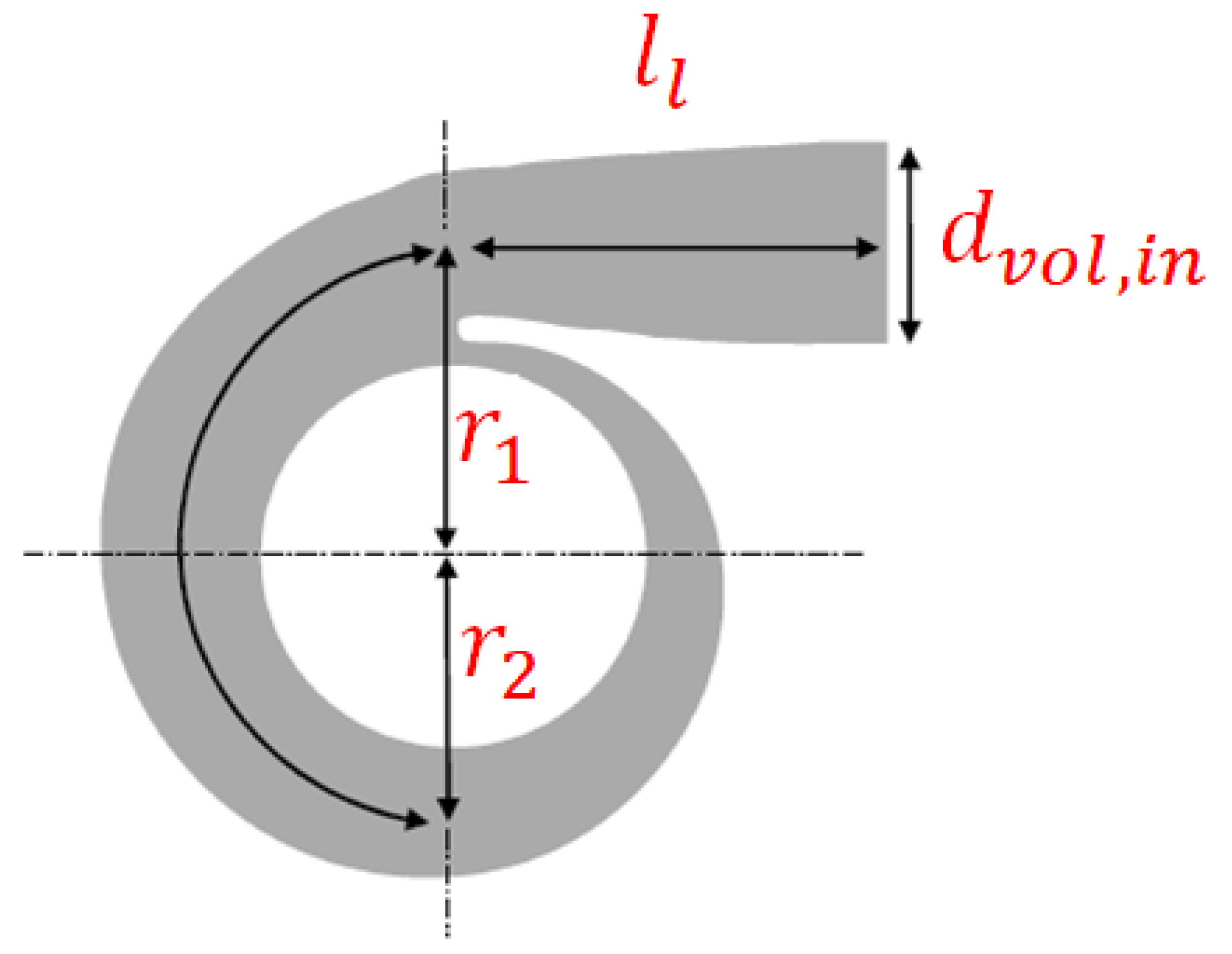
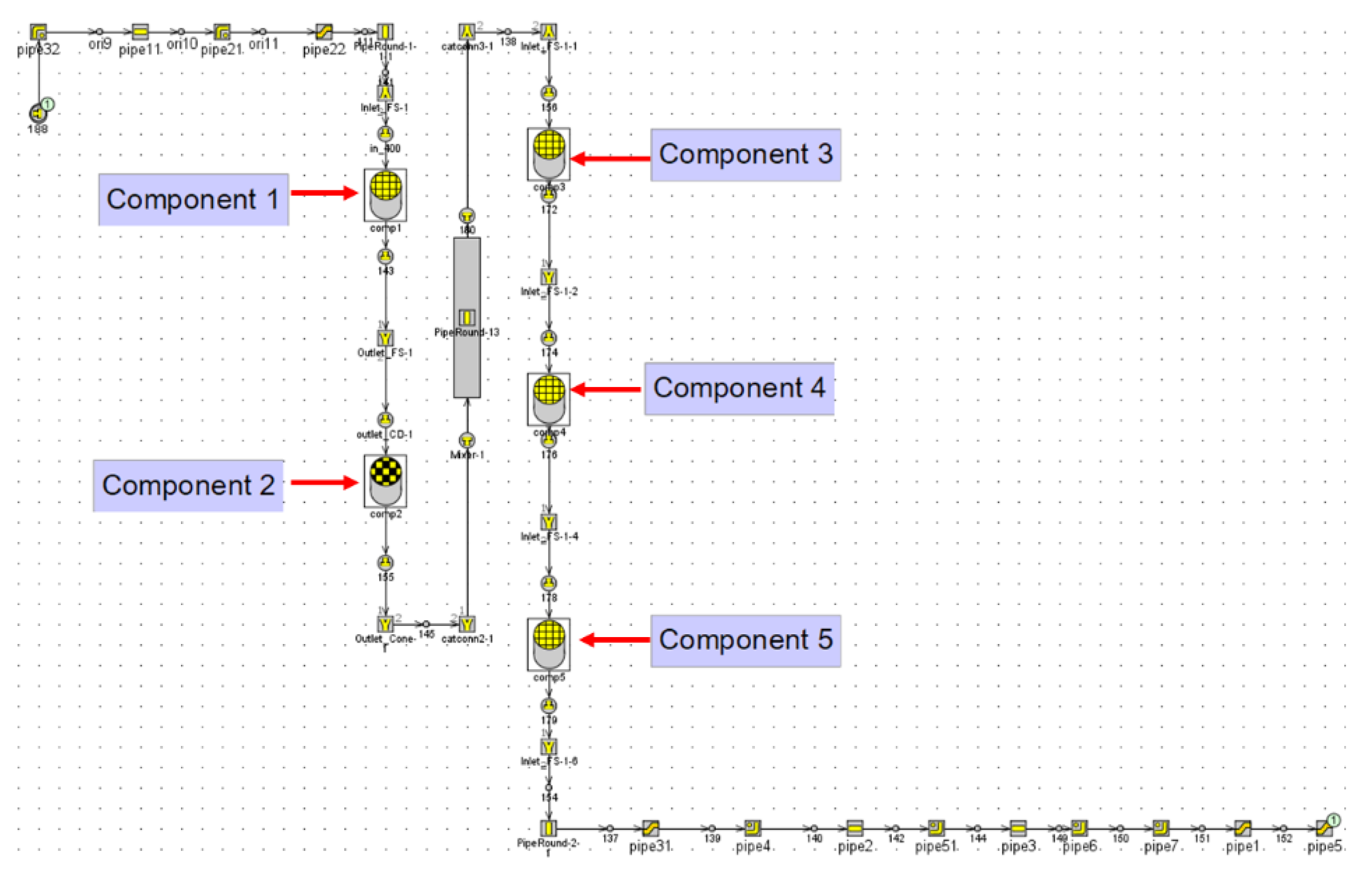
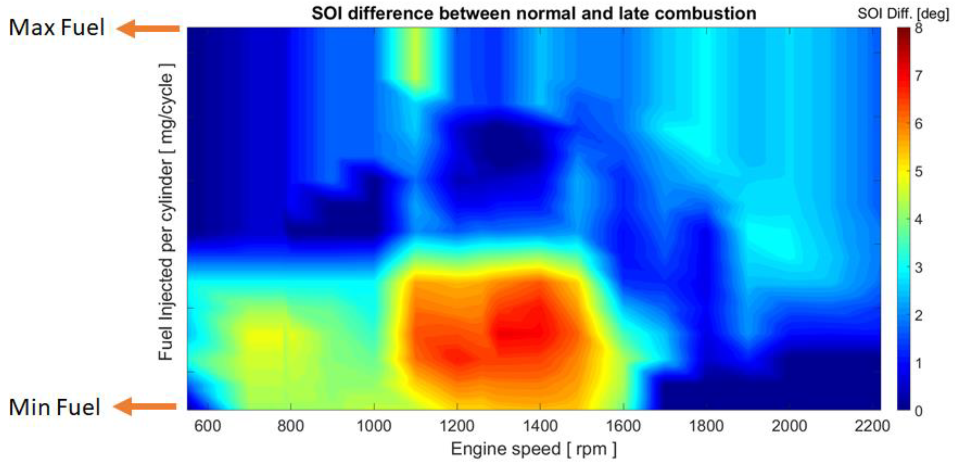
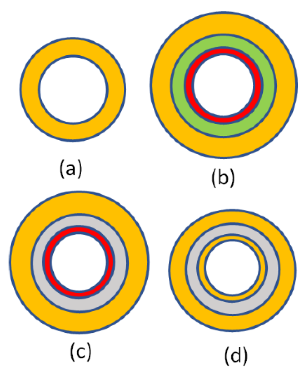
4.4. Thermal Insulation Analysis

As the SCR temperature approaches the target operating temperature, the flap actuation will be reduced and, once the target temperature is reached, combustion will be switched to the optimal mode. Preserving the available exhaust gas enthalpy through insulating the exhaust manifold, exhaust ports, and turbocharger (Figure 22 and Figure 23) should make it possible to reduce flap activation and, thus, improve fuel consumption.
Since there were no experimental data available regarding the insulation material, we used the data available in [32,33].
Different thermal insulation layouts can be found in [32]. The actual insulation of the baseline, exhaust manifold, exhaust ports, and turbocharger is shown in Figure 22. The baseline exhaust manifold was made from cast iron (Figure 22a). We made the following assumptions about the insulation:
  • for the exhaust port, a Yttria-stabilized zirconia [34] is sandwiched between the inner stainless-steel liner and the external iron structure (Figure 22b);
  • for the exhaust manifold, an air gap exists between the inner stainless-steel liner and the external iron manifold (Figure 22c); and
  • for the turbocharger, an external iron shield creates one air gap layer on the cast-iron turbine housing (Figure 22d).
The material properties that we used are shown in Table 3 [32]. It is worth noting that the values for thermal conductivities in the table are averages and the temperature-dependent thermal conductivity was used in the simulation.
In the final step of the analysis, the WHTC was simulated considering the insulation of different parts. The BSFC benefits are shown in Figure 24. Thermal insulation of the exhaust ports, exhaust manifold, and turbocharger leads to BSFC improvements of 0.5%, 0.24%, and 0.25%, respectively. In the ideal situation, if the SCR could be maintained at a temperature higher than the minimum threshold over the entire cycle, and thus always be in the optimal combustion mode, a maximum fuel saving of 3.2% over the baseline is possible. This is the maximum possible benefit using various technologies, such as catalytic heating.

5. Conclusions and Future Work

The aim of this study is to couple a 0D combustion model and an ECU model in order to correctly predict, under steady-state and transient conditions, the combustion trend, emissions, and other performance-related parameters of a heavy-duty diesel engine. Optimization of individual subsystems, such as the ICE, ATS, and control strategy, may not lead to the global optimal solution due to their complex interaction within the entire system. However, the holistic approach of physical models coupled with the real airpath ECU controls presented in this work increases the reliability of the predicted system performance and interactions. Such a tool could be utilized as a virtual test bench to better identify a system’s behavior in terms of emissions and engine performance. It could also be used to prepare the engineer before they go to the test bench, where an efficient use of time is critical to reducing development costs.
After careful validation of the engine model, the DIPulse predictive combustion model was calibrated using a DoE technique with the objective of minimizing the RMS error between the predicted and experimental burn rates. Additionally, the engine-out NOx emissions were predicted using the extended Zeldovich mechanism.
Subsequently, the ECU model, developed in the Simulink environment and validated during both transient and steady-state operation, was coupled with the engine model. The results show good agreement with measurements over a WHTC.
The coupled model was then used to predict the benefits of thermal insulation on the exhaust line in terms of fuel consumption during a hot WHTC. It was shown that insulation of the exhaust ports, exhaust manifold, and turbocharger leads to BSFC improvements of 0.5%, 0.24%, and 0.25%, respectively. A further simulation was carried out considering constant operation in the optimal combustion mode with a fully open exhaust flap. This analysis predicted a maximum achievable BSFC benefit using innovative technologies, such as catalytic heating, of about 3.2% over the baseline hot WHTC.
Future development of the work presented here will include an evaluation of the effectiveness of different thermal management technologies, such as VVA, catalytic heating, thermal insulation, intake flaps, and cylinder deactivation during a cold WHTC. Moreover, a fully calibrated ATS model, including chemical reactions, will be included in order to predict tailpipe NOx emissions in a fully integrated engine, controls, and ATS analysis.
Finally, due to its reduced computational and calibration requirements, the 0D/1D model developed in this study could be used as a “virtual test rig”, allowing for the evaluation of changes in hardware or software and their impact on the system from an early stage of engine development.

Author Contributions

Conceptualization, M.M. and S.L.; data curation, M.M.; formal analysis, M.M. and S.L.; funding acquisition, S.L.; Investigation, M.M. and S.L.; methodology, M.M. and S.L.; project administration, S.L.; software, M.M.; supervision, S.L.; validation, M.M. and S.L.; visualization, M.M.; writing—original draft, M.M.; writing—review & editing, M.M. and S.L. All authors have read and agreed to the published version of the manuscript.

Funding

This research was funded by FPT Industrial.

Acknowledgments

The authors would like to thank Philip Scarth, Giuseppe Cerada, and Oscar Chinellato for their precious and constant support as well as for their invaluable suggestions during the simulation activities.

Conflicts of Interest

The authors declare no conflict of interest.

Definitions and Abbreviations

Aftertreatment SystemATS
Brake Mean Effective PressureBMEP
Brake Specific Fuel ConsumptionBSFC
Computational Fluid DynamicsCFD
Design of ExperimentDoE
Diesel Oxidation CatalystDOC
Diffusion Combustion Rate MultiplierDCRM
Electronic Control UnitECU
Entrainment Rate MultiplierERM
European UnionEU
Exhaust Gas RecirculationEGR
Genetic AlgorithmGA
Ignition Delay MultiplierIDM
Internal Combustion EngineICE
Original Equipment ManufacturersOEMs
Premixed Combustion Rate MultiplierPCRM
Proportional, Integral and DerivativePID
Real Driving EmissionRDE
Root Mean SquaredRMS
Selective Catalytic ReductionSCR
Software in the LoopSiL
Start of InjectionSoI
Variable Geometry TurbochargerVGT
Variable Valve ActuationVVA
World Harmonized Transient CycleWHTC

References

  1. Johnson, T. Diesel emissions in review. SAE Int. J. Engines 2011, 4, 143–157. [Google Scholar] [CrossRef]
  2. Yamashita, A.; Ohki, H.; Tomoda, T.; Nakatani, K. Development of Low Pressure Loop EGR System for Diesel Engines; SAE Technical Paper 2011-01-1413; SAE International: Warrendale, PA, USA, 2011. [Google Scholar]
  3. Dittrich, P.; Peter, F.; Huber, G.; Kuehn, M. Thermodynamic Potentials of a Fully Variable Valve Actuation System for Passenger-Car Diesel Engines; SAE Technical Paper 2010-01-1199; SAE International: Warrendale, PA, USA, 2010. [Google Scholar]
  4. Piano, A.; Millo, F.; di Nunno, D.; Gallone, A. Numerical Assessment of the CO2 Reduction Potential of Variable Valve Actuation on a Light Duty Diesel Engine; SAE Technical Paper 2018-37-0006; SAE International: Warrendale, PA, USA, 2018. [Google Scholar]
  5. Burke, R.; Liu, Y.; Vijayakumar, R.; Werner, J.; Dalby, J. Inner-Insulated Turbocharger Technology to Reduce Emissions and Fuel Consumption from Modern Engines; SAE Technical Paper 2019-24-0184; SAE International: Warrendale, PA, USA, 2019. [Google Scholar]
  6. Pillai, S.; LoRusso, J.; van Benschoten, M. Analytical and Experimental Evaluation of Cylinder Deactivation on a Diesel Engine; SAE Technical Paper 2015-01-2809; SAE International: Warrendale, PA, USA, 2015. [Google Scholar]
  7. Millo, F.; Piano, A.; Paradisi, B.P.; Boccardo, G.; Mirzaeian, M.; Arnone, L.; Manelli, S. The Effect of Post Injection Coupled with Extremely High Injection Pressure on Combustion Process and Emission Formation in an Off-Road Diesel Engine: A Numerical and Experimental Investigation; SAE Technical Paper 2019-24-0092; SAE International: Warrendale, PA, USA, 2019. [Google Scholar]
  8. Rafigh, M. Exhaust Aftertreatment Modeling for Efficient Calibration in Diesel Passenger Car Applications. Ph.D. Thesis, Politecnico di Torino, Torino, Italy, 2017. [Google Scholar]
  9. Pfahl, U.; Schatz, A.; Konieczny, R. Advanced Exhaust Gas Thermal Management for Lowest Tailpipe Emissions-Combining Low Emission Engine and Electrically Heated Catalyst; SAE Technical Paper 2012-01-1090; SAE International: Warrendale, PA, USA, 2012. [Google Scholar]
  10. Cloudt, R.; Willems, F. Integrated Emission Management strategy for cost-optimal engine-aftertreatment operation. SAE Int. J. Engines 2011, 4, 1784–1797. [Google Scholar] [CrossRef]
  11. Domeit, P.A.; Lang, O.; Schulz, R.; Weng, V. CFD Simulation of Diesel Injection and Combustion; SAE Technical Paper 2002-01-0945; SAE International: Warrendale, PA, USA, 2002. [Google Scholar]
  12. Zhang, K.; Xin, Q.; Mu, Z.; Niu, Z.; Wang, Z. Numerical simulation of diesel combustion based on n-heptane and toluene. Propuls. Power Res. 2019, 8, 121–127. [Google Scholar] [CrossRef]
  13. Li, G.; Sapsford, S.; Morgan, R. CFD Simulation of DI Diesel Truck Engine Combustion Using VECTIS.; SAE Technical Paper 2000-01-2940; SAE International: Warrendale, PA, USA, 2000. [Google Scholar]
  14. Lebas, R.; Mauviot, G.; le Berr, F.; Albrecht, A. A Phenomenological approach to model diesel engine combustion and in-cylinder pollutant emissions adapted to control strategy. IFAC Proc. Vol. 2009, 42, 32–39. [Google Scholar] [CrossRef]
  15. Payri, F.; Olmeda, P.; Martín, J.; García, A. A complete 0D thermodynamic predictive model for direct injection diesel engines. Appl. Energy 2011, 88, 4632–4641. [Google Scholar] [CrossRef]
  16. Gamma Technologies. GT-SUITE Engine Performance Application Manual; Gamma Technologies: Belgrad, Serbia, 2019. [Google Scholar]
  17. Piano, A.; Millo, F.; Boccardo, G.; Rafigh, M. Assessment of the Predictive Capabilities of a Combustion Model for a Modern Common Rail Automotive Diesel Engine; SAE International: Warrendale, PA, USA, 2016. [Google Scholar]
  18. Heywood, J. Internal Combustion Engines Fundamentals; Mcgraw-Hill International: New York, NY, USA, 1953; Volume 11.2. [Google Scholar]
  19. Gelso, E.R.; Dahl, J. Diesel engine control with exhaust aftertreatment constraints. IFAC-PapersOnLine 2017, 50, 8921–8926. [Google Scholar] [CrossRef]
  20. Martin, J.; Arnau, F.; Piqueras, P.; Auñon, A. Development of an Integrated Virtual Engine Model to Simulate New Standard Testing Cycles; SAE Technical Paper 2018-01-1413; SAE International: Warrendale, PA, USA, 2018. [Google Scholar]
  21. Baines, N.; Wygant, K.; Dris, A. The Analysis of heat transfer in automotive turbochargers. J. Eng. Gas Turb. Powertrans. 2010, 132, 042301. [Google Scholar] [CrossRef]
  22. Romagnoli, A.; Martinez-Botas, R. Heat Transfer on a Turbocharger Under Constant Load Points. In Proceedings of the 54th ASME Turbo Expo, Orlando, FL, USA, 8–12 June 2009. [Google Scholar]
  23. Romagnoli, A.; Martinez-Botas, R. Heat transfer analysis in a turbocharger turbine: An experimental and computational evaluation. Appl. Therm. Eng. 2012, 38, 58–77. [Google Scholar] [CrossRef] [Green Version]
  24. Cormerais, M.; Chesse, P.; Hetet, J.F. Turbocharger heat transfer modeling under steady and transient conditions. Int. J. Thermodyn. 2009, 12, 193–202. [Google Scholar]
  25. Serrano, J.; Olmeda, P.; Arnau, F.; Reyes-Belmonte, M.; Lefebvre, A. Importance of heat transfer phenomena in small turbochargers for passenger car applications. SAE Int. J. Eng. 2013, 6, 716–728. [Google Scholar] [CrossRef] [Green Version]
  26. Serrano, J.; Olmeda, P.; Arnau, F.; Dombrovsky, A.; Smith, L. Analysis and methodology to characterize heat transfer phenomena in automotive turbochargers. J. Eng. Gas Turb. Power 2015, 137, 021901. [Google Scholar] [CrossRef]
  27. Serrano, J.; Olmeda, P.; Arnau, F.; Dombrovsky, A. Turbocharger heat transfer and mechanical losses influence in pre-dicting engines performance by using one-dimensional simulation codes. Energy 2015, 86, 204–218. [Google Scholar] [CrossRef] [Green Version]
  28. Chen, H.; Hakeem, I.; Martinez-Botas, R.F. Modelling of a Turbocharger Turbine under Pulsating Inlet Conditions. Proceedings of the Institution of Mechanical Engineers, Part A. J. Power Energy 1996, 210, 397–408. [Google Scholar] [CrossRef]
  29. Aymanns, R.; Scharf, J.; Uhlmann, T.; Lückmann, D. A revision of quasi steady modelling of turbocharger turbines in the simulation of pulse charged engines. Motortechnisch. Z. 2012, 55, 149–163. [Google Scholar]
  30. Millo, F.; Pautasso, E.; Delneri, D.; Troberg, M. A DoE Analysis on the Effects of Compression Ratio, Injection Tim-ing, Injector Nozzle Hole Size and Number on Performance and Emissions in a Diesel Marine Engine; SAE Technical Paper 2007-01-0670; SAE International: Warrendale, PA, USA, 2007. [Google Scholar]
  31. Mirzaeian, M.; Millo, F.; Rolando, L. Assessment of the Predictive Capabilities of a Combustion Model for a Modern Downsized Turbocharged SI; SAE Technical Paper 2016-01-0557; SAE International: Warrendale, PA, USA, 2016. [Google Scholar]
  32. Martin, J.; Serrano, J.; Piqueras, P.B. Diesel, Turbine and exhaust ports thermal insulation impact on the engine efficiency and aftertreatment inlet temperature. Appl. Energy 2019, 240, 409–423. [Google Scholar]
  33. Serrano, J.; Piqueras, P.; Navarro, R.; Gómez, J.; Marc, M.; Benedicte, T. Modelling Analysis of Aftertreatment Inlet Temperature Depend-ence on Exhaust Valve and Ports Design Parameters; SAE Technical Paper 2016-01-0670; SAE International: Warrendale, PA, USA, 2016. [Google Scholar]
  34. Viazzi, C.; Deboni, A.; Ferreira, J.Z.; Bonino, J.P.; Ansart, F. Synthesis of Yttria Stabilized Zirconia by sol–gel route: Influence of experimental parameters and large scale production. Solid State Sci. 2006, 8, 1023–1028. [Google Scholar] [CrossRef] [Green Version]
Figure 1. Experimental test matrix.
Energies 14 00652 g001
Figure 2. Model layout with the engine, turbocharger, and aftertreatment.
Energies 14 00652 g002
Figure 3. Heat transfer path from turbocharger to coolant and environment.
Energies 14 00652 g003
Figure 4. The 0D heat transfer model from turbocharger to coolant and environment.
Energies 14 00652 g004
Figure 5. Simplified representation of the turbine volute geometry [16].
Energies 14 00652 g005
Figure 6. Aftertreatment line layout.
Energies 14 00652 g006
Figure 7. Schematic presentation of the Electronic Control Unit (ECU) model coupled to the GT-Suite power engine model.
Energies 14 00652 g007
Figure 8. Comparison between measured and simulated in-cylinder pressure (a) and burn rate (b).
Energies 14 00652 g008
Figure 9. Percentage error between experimental and simulated values of Brake Specific Fuel Consumption (BSFC) (a) and air flow rate (b).
Energies 14 00652 g009
Figure 10. Error between experimental and simulated values of temperature before turbine operation (a) and temperature after turbine operation (b).
Energies 14 00652 g010
Figure 11. Error between experimental and simulated values of peak cylinder pressure (a) and turbocharger speed (b).
Energies 14 00652 g011
Figure 12. Comparison between experimental and simulated engine-out NOx.
Energies 14 00652 g012
Figure 13. Operating parameters of the engine during transient operation at 900 rpm.
Energies 14 00652 g013
Figure 14. Operating parameter of the engine during transient operation at 1900 rpm.
Energies 14 00652 g014
Figure 15. Comparison of simulated and experimental engine speed (a), torque (b), temperature before diesel catalyst oxidation (c), and selective catalytic reduction (SCR) temperature (d).
Energies 14 00652 g015
Figure 16. Comparison of experimental and simulated pressure after compression (a), pressure after flap opening, (b) air trapped at each cylinder (c), and fuel trapped per cylinder (d).
Energies 14 00652 g016
Figure 17. Comparison of experimental and simulated main Start of Injection (SOI) (a), injection pressure (b), engine-out NOx (c), and flap position (d).
Energies 14 00652 g017
Figure 18. Difference in SOI between normal and late combustion.
Energies 14 00652 g018
Figure 19. Comparison of simulated and experimental cumulative injected fuel during the World Harmonized Transient Cycle (WHTC).
Energies 14 00652 g019
Figure 20. Comparison of simulated and experimental cumulative power during the WHTC.
Energies 14 00652 g020
Figure 21. Comparison of simulated and experimental cumulative engine-out NOx during the WHTC.
Energies 14 00652 g021
Figure 22. (a) Baseline, (b) exhaust port insulation, (c) exhaust manifold insulation, and (d) turbocharger insulation.
Energies 14 00652 g022
Figure 23. Insulated parts in the model: exhaust port, exhaust manifold, and turbocharger.
Energies 14 00652 g023
Figure 24. BSFC benefits obtained by insulating the exhaust manifold, turbocharger, and exhaust ports.
Energies 14 00652 g024
Table 1. Main characteristics of the test engine.
Engine Characteristics
Bore128
Stroke144
N° cylinders6
Displacement11 L
Peak Power370 kW @1900 rpm
Peak Torque2360 Nm @1000 rpm
Valvetrain4 valves per cylinder
Table 2. Optimized values of the combustion model’s calibration parameters.
Calibration ParametersValue
ERM1.86
IDM0.35
PCRM0.85
DCRM0.65
Table 3. Material properties [32].
MaterialColorDensity ( k g m 3 ) Thermal Conductivity ( W m · K ) Surface Emissivity (–]
Stainless-steelRed790025.40.85
AirGray1.160.0667
YSZGreen4950 [1]1.0 [1]0.729
IronYellow787069.50.8
Publisher’s Note: MDPI stays neutral with regard to jurisdictional claims in published maps and institutional affiliations.

