An Improved Variational Mode Decomposition and Its Application on Fault Feature Extraction of Rolling Element Bearing

Abstract

The fault diagnosis of rolling element bearing is of great significance to avoid serious accidents and huge economic losses. However, the characteristics of the nonlinear, non-stationary vibration signals make the fault feature extraction of signal become a challenging work. This paper proposes an improved variational mode decomposition (IVMD) algorithm for the fault feature extraction of rolling bearing, which has the advantages of extracting the optimal fault feature from the decomposed mode and overcoming the noise interference. The Shuffled Frog Leap Algorithm (SFLA) is employed in the optimal adaptive selection of mode number K and bandwidth control parameter α. A multi-objective evaluation function, which is based on the envelope entropy, kurtosis and correlation coefficients, is constructed to select the optimal mode component. The efficiency coefficient method (ECM) is utilized to transform the multi-objective optimization problem into a single-objective optimization problem. The envelope spectrum technique is used to analyze the signals reconstructed by the optimal mode components. The proposed IVMD method is evaluated by simulation and practical bearing vibration signals under different conditions. The results show that the proposed method can improve the decomposition accuracy of the signal and the adaptability of the influence parameters and realize the effective extraction of the bearing vibration signal.

1. Introduction

As the key component of rotating machinery, the rolling bearings play an important role in the rotating machinery of modern industry. The running condition of the rolling element bearing is directly associated with the safety of the rotating machine [1,2]. However, the rolling element bearings are easily damaged under the long-term operation of a harsh environment with high speed, heavy load, and strong impact. The mechanical faults may cause the deterioration of operating conditions, resulting in serious economic losses and casualties [3,4,5]. The detected vibration signal is always related to the rich measurement information that a series of shock pulses will occur when the rolling bearing is subjected to a local failure [6,7]. However, the pulses caused by the defects in practice are too weak to distinguish the essential characteristic from a vibration signal corrupted by a large amount of background noise. Therefore, it is essential to remove the noise and extract the intrinsic features from the measured signal for the fault diagnosis of a rolling bearing.

Many vibration-based signal analysis methods have been researched and developed, where the feature extraction methods in time-domain such as probability analysis, correlation function method, synchronous averaging method [8], frequency-domain method such as spectrum analysis, cepstrum analysis, envelope analysis [9], and time–frequency domain features such as short-time Fourier transform (STFT), Wigner–Viller distribution (WVD), wavelet transform (WT), and its extension method, etc. [10]. Due to the inherent limitations of the method, the STFT method cannot get a high resolution in the time–frequency domain when dealing with the non-stationary signals. The disadvantage of the WVD method is that it cannot guarantee non-negative, especially for the multi-component signals or the complex modulation signals, there will be serious cross-term interference. The WT method decomposes the signal by performing scaling and translation operations on the wavelet basis. It has a good localization properties and multi-resolution analysis features in the time–frequency domain [11,12]. However, the high frequency band cannot be accurately split by the WT, which always exist the modulation information the faulty bearing. The wavelet packet transform (WPT) is an improved method based on WT, which divides the frequency-domain into various parts and allows a better time–frequency localization of signals [13]. Second generation wavelet transforms (SGWT) is a new wavelet construction method using the lifting scheme [14]. The time–frequency resolution of the SGWT method varies with the decomposition levels. It provides a good time and poor frequency resolution at high frequency sub-band and a good frequency and poor time resolution at low frequency sub-band [15].

Compared to the conventional time–frequency analysis methods, Empirical Mode Decomposition (EMD) method is a new adaptive signal processing method. It is suitable for the analysis of the nonlinear and non-stationary signals [16,17,18]. The EMD method can decompose the signal into a series of intrinsic mode functions (IMFs), which is built on the local characteristic time scales through performing a series of recursive calculations. The IMFs is characterized by the fundamental oscillatory modes of the signal, which makes the instantaneous frequency have the practical physical meaning. Therefore, the EMD method has received more attention for its application in the condition identification and the fault diagnosis of the rolling element bearings [19,20,21,22,23,24]. However, the EMD method has the phenomenon of the mode mixing caused by the intermittent signals when dealing with the non-linear and non-stationary signals. The Ensemble EMD (EEMD) with the noise assisted method was developed, which can eliminate the mode mixing by adding white noise [25,26]. However, this method also generated a new problem, which tolerates the residual noise in the signal reconstruction. The complementary ensemble empirical mode decomposition (CEEMD) is an improved algorithm of noise enhanced data analysis method. The residue of added white noise can be extracted by the pairs of complementary ensemble IMFs with positive and negative added white noise in this approach. It effectively eliminated the residual noise in the IMFs [27,28].

Variational mode decomposition (VMD) method has been proposed and developed recently, which is an alternative non-recursive signal decomposition method that can adaptively determine the relevant frequency bands and the corresponding mode simultaneously [29,30,31]. The VMD method decomposes a signal into a series of band-limited modes. These modes can be continuously updated with Wiener filtering, and the central frequency of each mode can be gradually demodulated to the corresponding baseband [19]. The non-recursive signal decomposition of VMD is more efficient than the EMD and its extension forms in computation. At the same time, the application of Wiener filtering makes the VMD method robust to the background noise. Due to the application of Wiener filters, the narrow-banded function of VMD resultant modes not only reduces the mode mixing issues existing in the EMD but also helps to accurately extract the fault characteristics of the signal through the Hilbert transform. However, the decomposition accuracy of the VMD method is usually affected by the mode number k and the bandwidth control parameter α. The original VMD used the default values to implement the signal analysis, which largely limits its decomposition precision and feature extraction capability.

In this paper, an improved fault feature extraction algorithm based on VMD is presented. The Shuffled Frog Leap Algorithm (SFLA) is employed to carry out the optimal adaptive selection of mode number k and the bandwidth control parameter α. A multi-objective evaluation function, which is built on the envelope entropy, the kurtosis and the correlation coefficients, is constructed to select the optimal mode component. The efficiency coefficient method (ECM) is utilized to transform the multi-objective optimization problem into a single-objective optimization problem. The optimal modal component is reconstructed and processed by the spectrum analysis method. The rest of the paper is organized as following. Section 2 gives the theoretical background of the VMD and SFLA. Section 3 provides the improved variational mode decomposition (IVMD) method, which is based on SFLA and the objective optimization function of multi-parameter fusion. Section 4 presents the basic framework of the proposed method for signal analysis. Section 5 verifies the effectiveness of the proposed method in the feature extraction for the bearing fault diagnosis. Finally, the conclusions are drawn in Section 6.

2. Basic Theory

2.1. Variational Mode Decomposition

VMD is a new adaptive and quasi-orthogonal signal processing method [29], through which an input signal $f\left(t\right)$ can be decomposed into a limited number of IMFs. By solving the optimal solution of the constrained variational problem, the central frequency and band-limited of each mode can be decided. An input signal $f\left(t\right)$ can be expressed as following:

$$f\left(t\right)={\displaystyle \sum }_{k=1}^K{u}_k\left(t\right)$$

(1)

where $k$ represents the decomposition number of IMFs. $u_k\left(t\right)$ is the narrow-band mode function.

The VMD method decomposes the input signal into a certain number of modes, which make them reappear the input signal and have specific sparsity properties. It assumes each mode closely integrates around the center frequency. To assess the bandwidth of a mode, the following scheme is needed: (1) Compute the analyzed signal by the Hilbert transform to get a one-sided frequency spectrum for the mode $u_k$. (2) Transform the frequency spectrum of each mode to the baseband by mixing with an exponential tuned to the estimated center frequency. (3) Estimate the bandwidth through the H¹ Gaussian smoothness of the demodulation signal, that is, the squared L²-norm of the gradient. The constrained variational problem can be expressed as following:

$$\underset{\left\{u_k\right\},\left\{{\omega }_k\right\}}{min}\left\{{\displaystyle \sum }_k\Vert {\partial }_t\left[\left(\delta \left(t\right)+\frac{j}{\pi t}\right)\ast u_k\left(t\right)\right]e^{-j{\omega }_{k}t}{\Vert }_2^2\right\}, s.t.{\displaystyle \sum }_k{u}_k\left(t\right)=f\left(t\right)$$

(2)

where $\left\{u_k\right\}=\left\{u_1,u_2,\cdots ,u_K\right\},$ K denotes the number of the IMF component by the decomposition, ${\omega }_{k }\left(k=1,2,\cdots ,K\right)$ represents the central frequency of the k-th IMF, ${\partial }_t$ is the partial derivative function, and $\delta \left(t\right)$ Is the unit pulse function.

To transform the constrained variational problem into unconstrained problem, the quadratic penalty factor and Lagrange multiplier are introduced, and then the augmented variational problem is gotten by

$$L(\left\{u_k\right\},\left\{{\omega }_k\right\},\lambda )=\alpha {{\displaystyle \sum _k\Vert {\partial }_t\left[(\delta (t)+\frac{j}{\pi t})u_k(t)\right]e^{-j{\omega }_{k}t}\Vert }}_2^2+{\Vert f(t)-{\displaystyle \sum _k{u}_k(t)}\Vert }_2^2+\langle \lambda (t),f(t)-{\displaystyle \sum _k{u}_k(t)}\rangle$$

(3)

where $\alpha$ denotes the quadratic penalty factor (i.e., the bandwidth control parameter). $\lambda$ is the Lagrange multiplier.

To solve the variational problem, the alternate direction method of multipliers (ADMM) is applied to the Equation (3) by optimizing the parameters $u_k \mathrm{and} {\omega }^k$. The optimization of $u_k \mathrm{and} {\omega }^k$ are established by Equations (4) and (5), respectively.

$$u_k^{k+1}=\underset{u_k}{min}\left\{\alpha \Vert {\partial }_t\left[\left(\delta \left(t\right)+\frac{j}{\pi t}\right)\ast u_k\left(t\right)\right]e^{-j{\omega }_{k}t}{\Vert }_2^2+\Vert f\left(t\right)-{\displaystyle \sum }_i{u}_i\left(t\right)+\frac{\lambda \left(t\right)}{2}{\Vert }_2^2\right\}$$

(4)

$${\omega }_k^{k+1}=\underset{{\omega }_k}{min}\{\Vert {\partial }_t\left[\left(\delta \left(t\right)+\frac{j}{\pi t}\right)\ast u_k\left(t\right)\right]e^{-j{\omega }_{k}t}{\Vert }_2^2\}$$

(5)

The iterative equations of the mode and the center frequency can be obtained in the frequency domain by solving Equations (4) and (5), and are represented as follows:

$$u_k^{n+1}\left(\omega \right)=\frac{f\left(\omega \right)-{\sum }_{i\ne k}u\left(\omega \right)+\frac{\lambda \left(\omega \right)}{2}}{1+2\alpha {(\omega -{\omega }_k)}^2}$$

(6)

$${\omega }_k^{n+1}=\frac{{\int }_0^{\infty }\omega {\left|u_k\left(\omega \right)\right|}^{2}d\omega }{{\int }_0^{\infty }{\left|u_k\left(\omega \right)\right|}^{2}d\omega }$$

(7)

The Lagrange multipliers $\lambda$ can be updated as follows:

$${\lambda }^{n+1}\left(\omega \right)={\lambda }^n\left(\omega \right)+\tau \left(f\left(\omega \right)-{\displaystyle \sum }_k{u}_k^{n+1}\left(\omega \right)\right)$$

(8)

The calculation processes of VMD are the following:

Step 1: Initialize: $\left\{u_k^1\right\}$, $\left\{{\omega }_k^1\right\}$, ${\lambda }^1$ and $n=1$;

Step 2: Start iteration, $n=n+1;$

Step 3: Update $u_k$ and ${\omega }_k$ according to Equations (6) and (7);

Step 4: Update the Lagrange multipliers $\lambda$ using Equation (8);

Step 5: For a given accuracy $\epsilon$, if $\sum _k\Vert u_k^{n+1}-u_k^n{\Vert }_2^2<\epsilon$, stop the iteration, else turn to Step 2.

2.2. Shuffled Frog Leaping Algorithm

Shuffled frog leaping algorithm (SFLA) is a novel heuristic population evolution algorithm. It combines the advantages of both the genetic-based memetic algorithm (MA) and the social behavior-based the particle swarm optimization algorithm [32,33,34]. Compared with the traditional optimization algorithms, SFLA has a superior ability of global optimization and fast convergence.

Suppose a population of frogs $N_{pop}$ is randomly generated within the S-dimensional space. The i-th frog is expressed by variables $S$ as $X_i=\left(x_{i1},x_{i2},\cdots ,x_{iS}\right)$. Based on their self-fitness, the frogs are sorted by descending order. Thereafter, the population $N_{pop}$ is divided into $N_m$ subsets. The subsets are referred to as the memeplexes. Each memeplex contains $N_n$ frogs (i.e., $N_{pop}=N_m\times N_n$). In this process, the first frog goes to the first memeplex, the second frog goes to the second memeplex, the $m$ frog goes to the m-th memeplex, the $m+1$ frog goes back to the first memeplex, and so forth. Assuming that $M^k$ is a set of frogs for the k-th memeplex, the allocation process can be expressed as follows:

$$M^k=\left\{X_{k+m\left(l-1\right)}\in P|1\le l\le n\right\}, 1\le l\le m$$

(9)

For each memeplex, the frog with the best fitness is defined as $X_b$, the frog with the worst fitness is defined as $X_{\omega }$, and the frog with the global best fitness is defined as $X_g$. An evolutionary process is used to improve the worst fitness frog (i.e. not all frogs) in each cycle. Accordingly, the position of the frog with the worst fitness can be adjusted as the following:

$$D_i=Rand\times \left(X_b-X_{\omega }\right)$$

(10)

$${X^{\prime }}_{\omega }=X_{\omega }+D_i,\Vert D\Vert \le D_{max}$$

(11)

where $D_{max}$ expresses the maximum allowable change in the position of a frog.

If the process of evolution produces a better frog, it will replace the worst frog. Otherwise, the computations in Equations (10) and (11) will be repeated to get the global best frog (i.e., $X_g$ replaces $X_b$). If there is no improvement in this case, a new solution will be randomly generated to replace the worst frog with another frog having an arbitrary fitness. The computations will continue for a specific number of evolutionary iterations within each memeplex. Therefore, SFLA simultaneously implements an independent local search in each memeplex using a process similar to the particle swarm optimization algorithm [35].

After a predefined number of memetic evolutionary steps within each memeplex, the solutions of evolved memeplexes $\left\{X_1,X_2,\cdots ,X_P\right\}$ Are replaced in the new population, this is called the shuffling process. The shuffling process promotes global information exchange among the frogs. Then, the population is sorted in order of decreasing value and updates the population best frog’s position $X_g$, repartition the frog group into memeplexes, and progress the evolution within each memeplex until the conversion criteria are satisfied. Usually, the convergence criteria can be defined as follows [31]:

• The relative change in the fitness of the global frog within a number of consecutive shuffling iterations is less than a pre-specified tolerance.
• The maximum predefined number of shuffling iterations has been obtained.

3. Improved VMD Algorithm

To process of nonlinear vibration signal using the VMD algorithm, the selection of the mode number K and the bandwidth control parameter α has a greater impact on the decomposition result. A smaller α will result in a larger bandwidth of the IMF component. Conversely, there is a smaller bandwidth of the IMF component. The excessive selection of the mode number will produce the redundant components. While a small mode number will lead to the mode aliasing. On the other hand, a wider filter bandwidth will make more noise and interference information into the decomposition results. Narrow filter bandwidth will lead to the lack of important information. To improve the accuracy of signal decomposition, SFLA is utilized to search for the optimal combination of influencing parameters, which can avoid the intervention of the subjective factors and automatically screen out the best combination of influence parameters. The multi-objective evaluation function is constructed for the selection of the optimal mode component. The efficiency coefficient method (ECM) is utilized to transform the multi-objective optimization problem into a single-objective optimization problem.

Suppose that the population composed of $N_{pop}$ frogs is $X$ in D dimensional space, $N_{pop}$ frogs are divided into $N_m$ subgroups through the descending order. The best individual $p_b$ and the worst individual $p_w$ in the subgroup can be calculated. Group optimal solution $S_1$ in the maximum number of iterations $M$ can be expressed as follows:

$$S_1=A\times \left(p_b-p_w\right)$$

(12)

When SFLA is utilized to optimize the influencing parameters, every update of the frog is performed by comparing the fitness value. Therefore, a fitness objective function should be established.

Shannon entropy can represent the amount of chaos owing to the many uncertainties within a system; the disorder is greater in a system. The greater is its randomness and the higher is its entropy value. The vibration signals of rolling element bearings have the characteristics of the uncertainty, the non-linearity, and the non-stationarity, and the entropy can be used as a feature indicator to measure complex signals and signals with the uncertain status of distribution [36]. The envelope signal after the demodulation is processed through a probability distribution sequence $p_i$. The envelope entropy $E_p$ of the signal $x_i$ could be expressed as following:

$$\begin{array}{c}{E}_p=-{\displaystyle {\displaystyle \sum }_{i=1}^N}{p}_i lg{p}_i\\ p_i=\frac{a\left(i\right)}{{\sum }_{i=1}^{N}a\left(i\right)}\end{array}\}$$

(13)

where $p_i$ is the normalization of $a\left(i\right)$, $a\left(i\right)$ is the obtained envelope signal by demodulating the signal $x_i$.

In the analysis and processing of the vibration signals, kurtosis is usually used to reflect the impact components in the signals and to describe the peak degree of the signals [37]. It is a dimensionless parameter. The calculation formula is as follows:

$$E=\frac{E\left(X-\mu \right)}{{\sigma }^4}$$

(14)

where $\sigma$ is the standard deviation of signals, $E\left(X\right)$ is the mathematical expression of signals, $\mu$ is the mean value of signals. A larger kurtosis value indicates that the signal contains more impact components. The kurtosis value is smaller, indicating that the signal is stable.

The correlation coefficient is often used in the vibration signal analysis, which reflects the degree of correlation between the two signals [38]. It can be expressed as

$${\rho }_{XY}=Corr\left(X,Y\right)=\frac{Cov\left(X,Y\right)}{\sqrt{D\left(X\right)}\sqrt{D\left(Y\right)}},\left|{\rho }_{XY}\right|\le 1$$

(15)

where $Cov\left(X,Y\right)$ is the covariance. $D\left(X\right)$ and $D\left(Y\right)$ are the variance of signal X and Y, respectively. The correlation coefficient is closer to 0, indicates that the correlation degree of the signals is lower. The absolute value of the correlation coefficient is closer to 1, indicates that the correlation degree of the signals is higher.

The multi-objective evaluation function is constructed for the selection of the optimal mode component and the calculation of fitness value, which is based on the envelope entropy, the kurtosis, and the correlation coefficients. When the i-th frog is located in the position $j$ (corresponding to a set of parameters ${\alpha }_j$ and $K_j$), the kurtosis, the correlation coefficient, and the envelope entropies of all mode components obtained by VMD process are all calculated. The components with the largest kurtosis value, the highest correlation and the smallest envelope entropy are selected and reconstructed as the fitness value in the optimization process.

In order to facilitate the operation of the SFLA, the efficacy coefficient method is used to convert the multi-objective function into a single objective function [39]. Each sub-objective function $f_i\left(X^{\left(k\right)}\right)$ can use an efficacy coefficient ${\eta }_i\left(0\le {\eta }_i\le 1\right)$ to express the quality of the objective. When ${\eta }_i=1$, it means that the effect of the i-th objective function is the best, and when ${\eta }_i=0$ means that the i-th objective function is the worst. The efficacy coefficient of the ith objective function at the data point $f_i\left(X^{\left(k\right)}\right)$ is defined as

$${\eta }_i=\frac{f_i\left(X^{\left(k\right)}\right)-f_{imin}\left(X\right)}{f_{imax}\left(X\right)-f_{imin}\left(X\right)}$$

(16)

where $f_{imin}\left(X\right)$ and $f_{imax}\left(X\right)$ are the minimum and maximum values under the constraints, respectively.

The efficacy coefficients of the kurtosis, the correlation, and the minimum envelope entropy obtained by the above formula are ${\eta }_K$, ${\eta }_C$ and ${\eta }_E$, respectively. The multi-objective optimization problem can be evaluated by the average of the efficacy coefficients. The total efficacy coefficient is expressed as $\eta =\sqrt[3]{{\eta }_E{\eta }_K{\eta }_C}$. Obviously, the value η is close to 1, indicates that the effect of the optimization is better. Conversely, when the value $\eta$ is close to 0, the optimization effect is worse.

When the improved VMD is used for the nonlinear and non-stationary vibration signal processing, the flowchart of the parameter optimization is shown in Figure 1, and the optimization steps are briefly described as the following:

• Initialize the parameters: total number of frogs $N_{pop}$, number of subgroups $N_m$, number of each group frogs $N_f$, maximal number of iterations $M$, random initialization of frog individuals, initialize the population;
• Implement VMD, and obtain a set of IMFs;
• Construct the global fitness function based on the envelope entropy, the kurtosis, and the correlation coefficients;
• Calculate the fitness value of each frog;
• Rank the frogs according to their fitness values;
• Divided the sorted frogs $N_{pop}$ into $N_m$ subgroups according to the descending order of the objective function. The first frog goes to the first memeplex, the second frog goes to the second memeplex, frog m goes to the m-th memeplex, and frog $m+1$ goes to the first memeplex, and so on.
• Determine the best individual of the subgroup $p_b$, the worst individual $p_w$ and the optimal solutions in the population $S_1$, the worst solution is improved by the Equation (12) in evolutional iterations $M$;
• Update the worst individual and descend the order to the individual to form a new group;
• Judge whether the algorithm satisfies the terminating condition, outputs the optimum solution when the algorithm satisfies the termination condition, otherwise moves on to step 6.

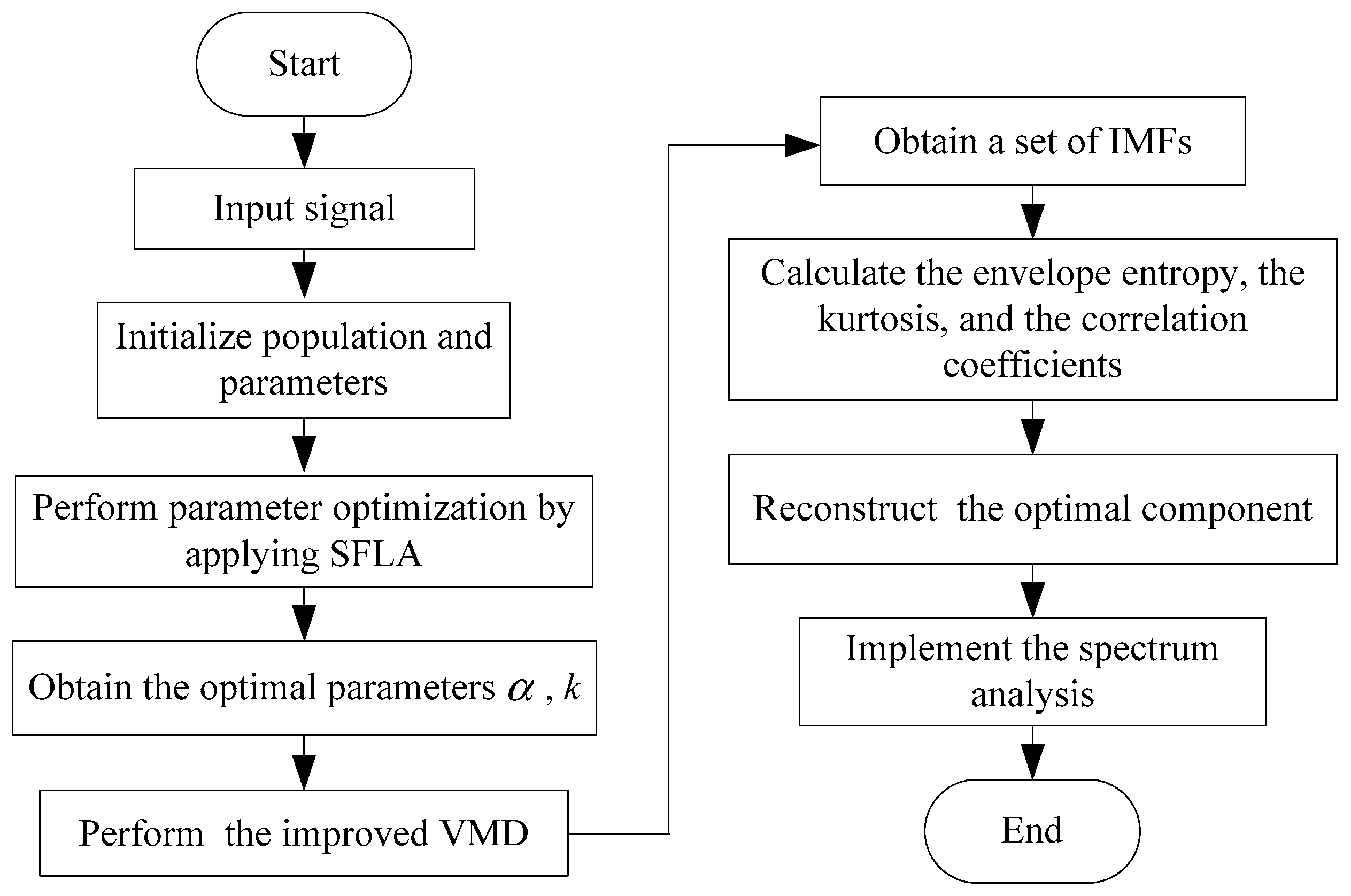
4. Fault Feature Extraction by IVMD

The periodic impact energy caused by the failure of the rolling bearing is weak, and it is relatively difficult to extract fault features due to the effects of noise and signal attenuation. When there is a fault for the rolling bearing, the useful characteristic components usually have very little energy, and it is submerged by the background noise. It is difficult to extract useful fault features. In order to extract the fault feature effectively and realize the fault diagnosis, the IVMD is presented to extract the useful fault features for the fault diagnosis of the rolling element bearing. The vibration signal is decomposed into a series of intrinsic mode functions by the IVMD algorithm. The envelope spectrum technique is utilized to analyze the best signal component. The fault features of the rolling bearing would be easily detected and extracted. The fault features extraction procedure of the IVMD method is briefly described as follows and Figure 2 is its flow chart.

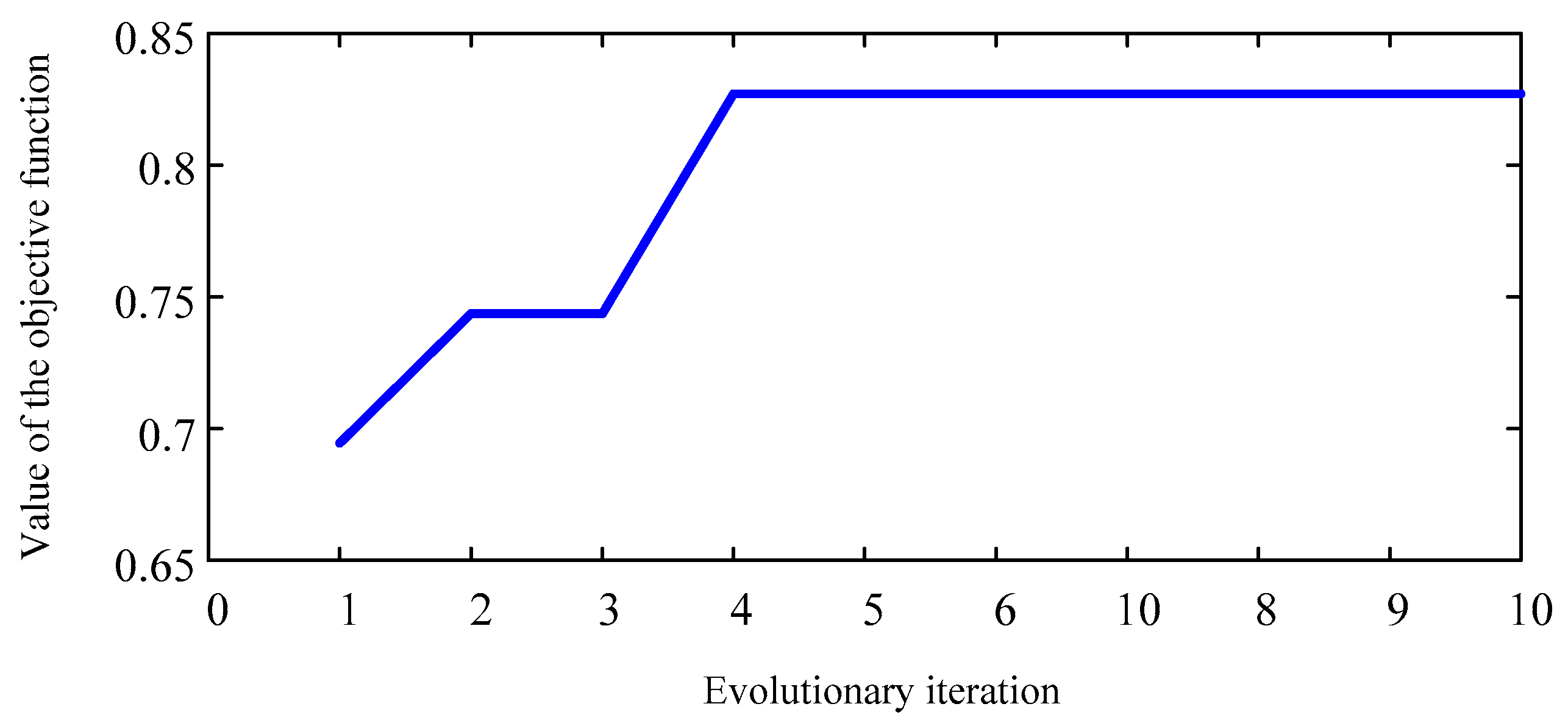
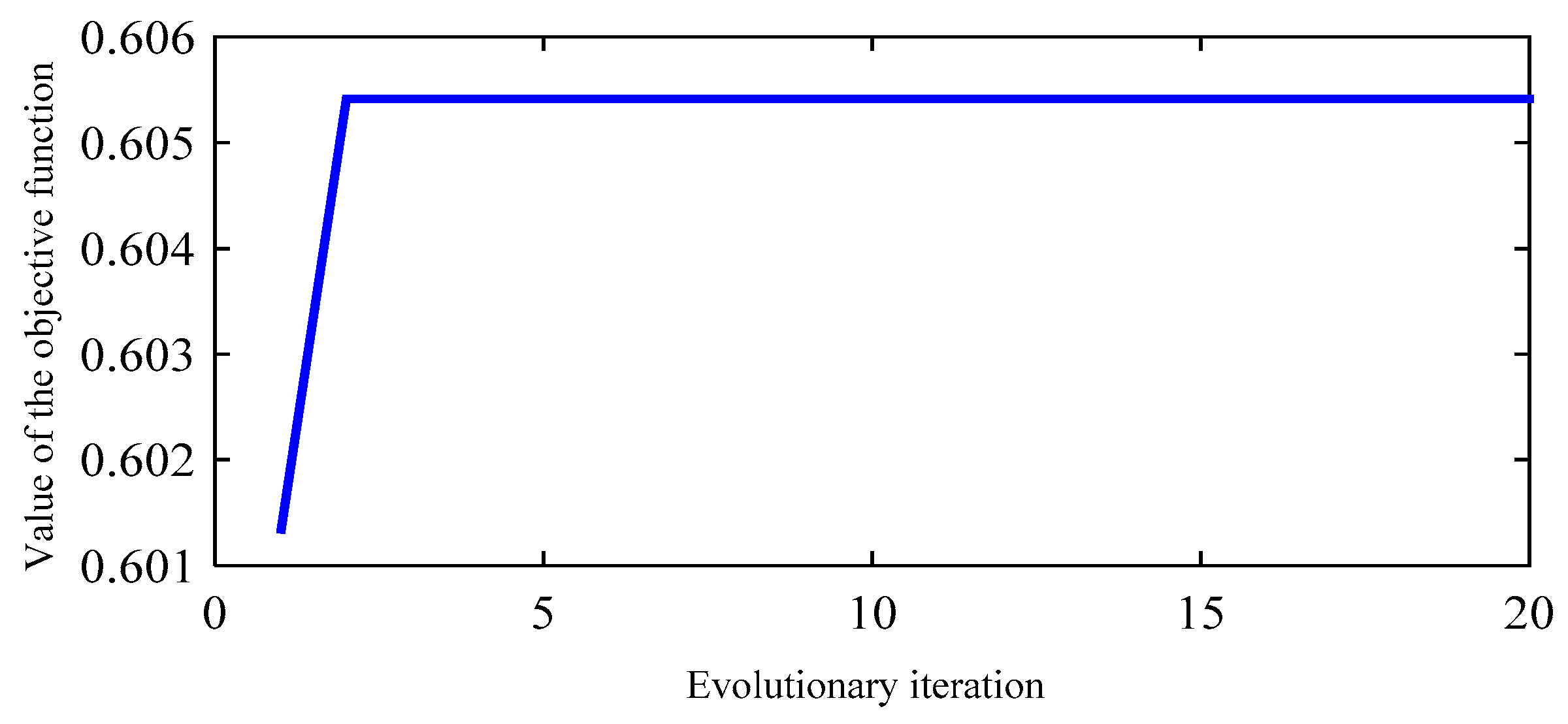
• Initialize population and parameters: the numbers of subgroup $N_m$, the numbers of each group frogs $N_f$, the numbers of iteration within a group $N_e$, the numbers of evolutional iteration $M$;
• Optimize VMD parameters by applying SFLA and obtain global optimal parameter k and $\alpha$;
• Decompose the original vibration signal into a set of the IMFs by the improved VMD;
• Calculate the envelope entropy, kurtosis and correlation coefficients of all IMF components;
• Select the reconstructed IMF component with the largest kurtosis value, the highest correlation and the smallest envelope entropy as the optimal component;
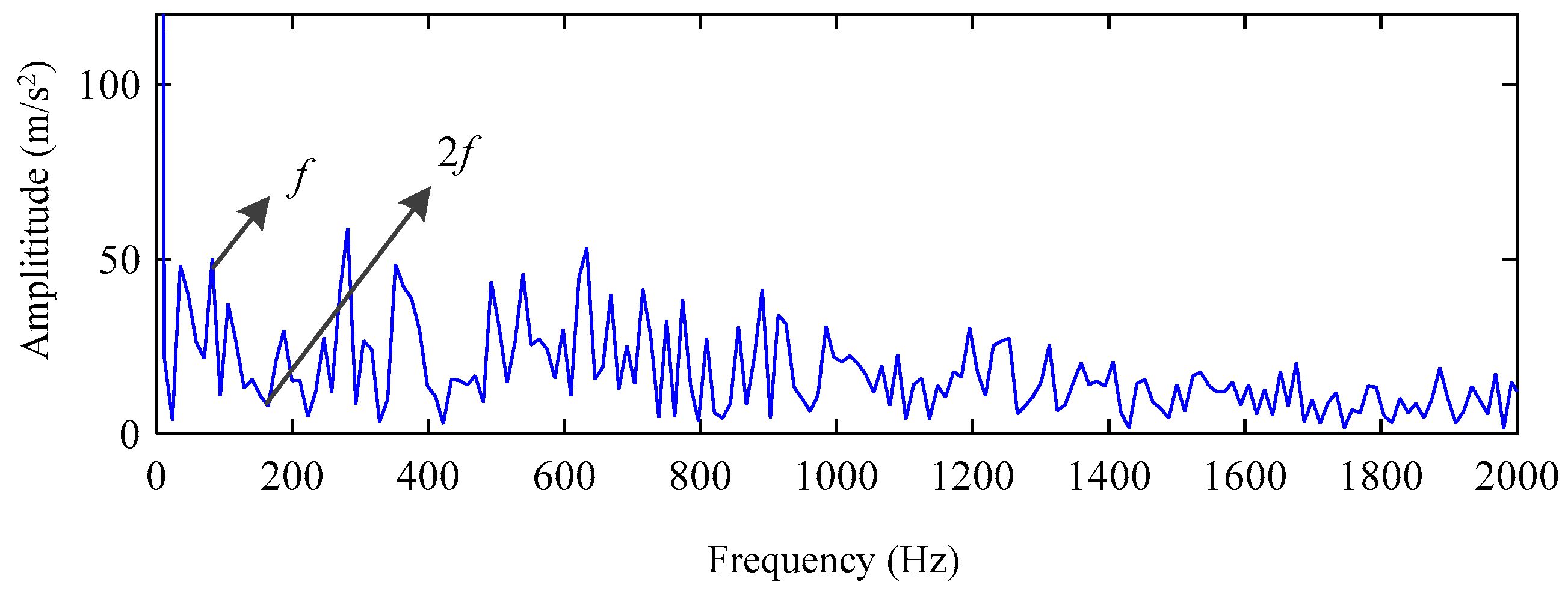
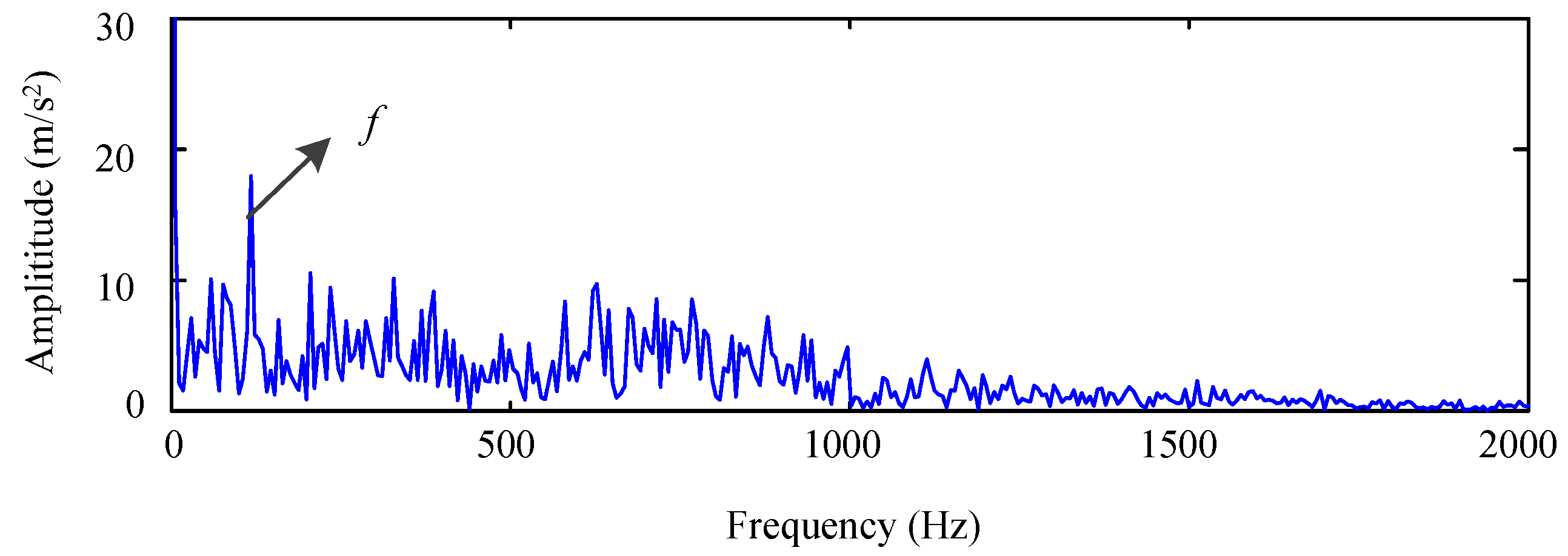
• Implement the spectrum analysis and compare the fault feature frequency in the envelope spectrum with the theoretical value of the bearing fault and determine the fault.

5. Experimental Results and Analysis

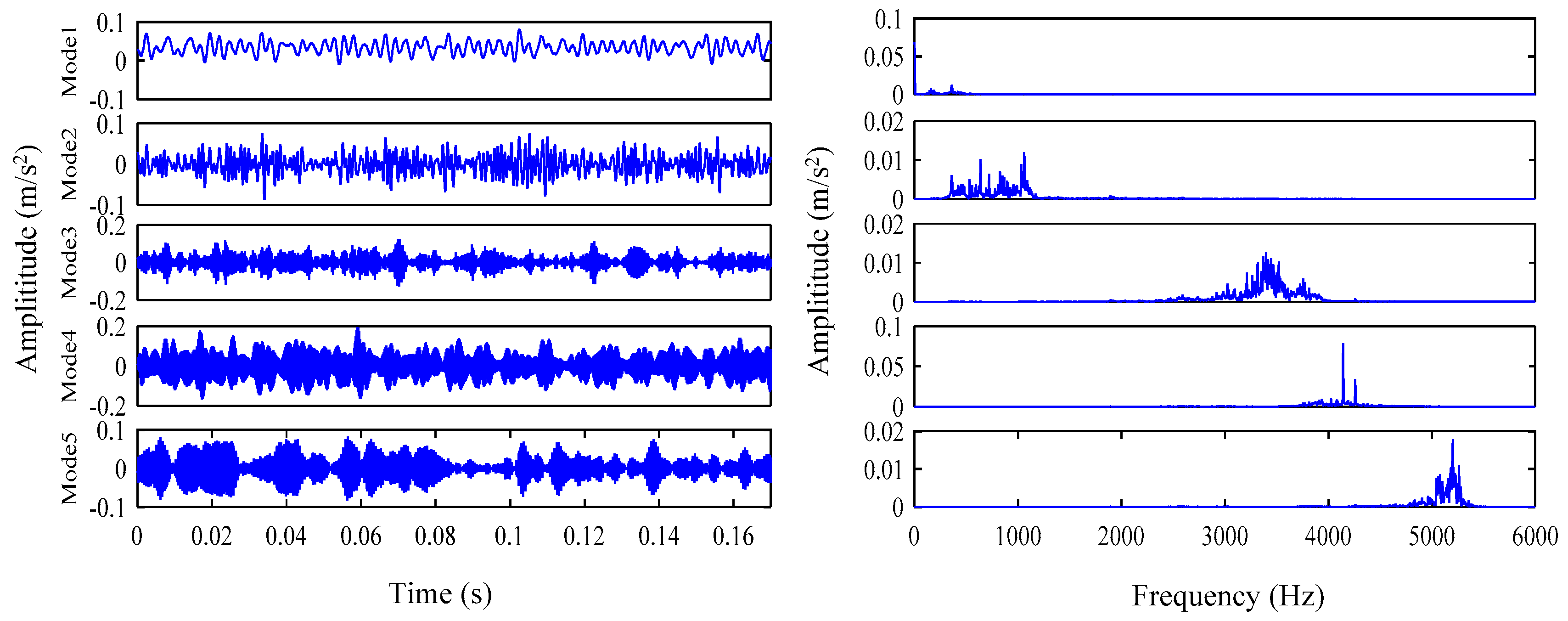
5.1. Simulation Analysis Using IVMD Algorithm

In order to quantitatively evaluate the feasibility of the IVMD method, the simulation signal of bearing fault is constructed. As we all know, the rolling element bearing failure will produce a series of pulse impact. Therefore, the simulation signal was mainly composed of the impact signal and noise signal generated by a bearing fault. The signal is sampled at 12 kHz. The simulated fault frequency $f_i$ is set to 80 Hz. The resonance frequency $f_n$ is set to 3 kHz. The rotating frequency $f_r$ is 20 Hz. The simulated signal is expressed as the following:

$$\begin{array}{c}x\left(t\right)=s\left(t\right)+n\left(t\right)={\displaystyle {\displaystyle \sum }_i}{A}_{i}h\left(t-iT-{\tau }_i\right)+n\left(t\right)\\ A_i=1+A_{0}sin(2\pi f_{r}t)\\ h\left(t\right)=e^{-Ct}sin(2\pi f_{n}t)\end{array}\}$$

(17)

where $h\left(t\right)$ is the generated waveform of a single impact, $A_i$ is the amplitude of the i-th impact force and considers possible periodic modulations, and $n\left(t\right)$ is the white Gaussian noise, Signal to noise ratio $R_{SNR}$ is −1 dB. $T$ is the mean spacing among impacts, the attenuation coefficient $C$ is 700, ${\tau }_i$ is the random variable.

The time-domain plot and the envelope spectrum of the simulated signal are shown in Figure 3. It can be seen from Figure 3 that the impact signal is submerged in the strong background noise in the simulated signal. The resonance frequency band of the spectrum is also not obvious. The frequency and period of the signal could not be found, and the feature frequency of the fault signals could not be accurately found from the envelope spectrum.

The simulated signal is decomposed by EMD, and the corresponding frequency spectrum is shown in Figure 4. Obviously, the useful frequency components could not be distinguished from the decomposed IMFs, and they are contaminated with noise. Many parts of IMF 1 are replaced by the intermittent pulse signal. The replaced parts of IMF 1 are shifted to IMF 2 resulting in the phenomenon of mode mixing in the second and all the following IMFs. In addition, as noted in Figure 4, the first three IMFs provided more information than the other IMFs, and the rest of the IMFs contain many redundant low-frequency components. In other words, the first three IMFs could be regarded as valid components of the signal, while the other IMFs were the low-frequency pseudo-components that can mislead the analysis of the signal.

The same simulated signal is decomposed by EEMD, CEEMD, VMD, and IVMD method, respectively. The decomposition results and corresponding frequency spectrums are presented in Figure 5, Figure 6, Figure 7 and Figure 8. It can be seen from Figure 4 and Figure 5 that the IMF 1 shows the mixture of the signals contaminated to a certain degree by adding noise. From the mode components and corresponding frequency spectrums shown in Figure 5 and Figure 6, it can be observed that the decomposition effect of EEMD and CEEMD was not much different from EMD. The feature frequency still could not be distinguished. The difference between EEMD and CEEMD of the decomposition results could be distinguished from the residuals. The residual of adding white noise is obviously smaller than EEMD. It is evident from Figure 9 that the residual amplitude of CEEMD signal was almost zero. Compared with the EEMD method, CEEMD added the white noise via pairs of complementary ensemble IMFs with positive and negative added white noise into the original signal. This method can effectively remove the white noise after decomposition and solve the problem of reconstruction error caused by the added auxiliary noise.

Compared with the decomposition results of EMD, EEMD, and CEEMD, the decomposition results of VMD and IVMD are better than the above methods. These two methods can effectively eliminate the phenomenon of mode mixing and suppress noise.

EMD, EEMD, and CEEMD methods use cyclic recursive sieving to obtain component signals. Therefore, the first component of the three methods contains abundant fault information and can be regarded as the optimal component. The envelope spectrum of their optimum components is shown by Figure 10, Figure 11 and Figure 12, respectively. It can be seen in the envelope spectrum of the optimal component shown in Figure 10, Figure 11 and Figure 12 that the characteristic frequency of the fault signal could not be accurately extracted, and there are the pseudo components. The mode component corresponding to the optimal component by using the VMD method is mode 4. The envelope spectrum of the optimal component is shown as Figure 13. It was the same as the decomposition results of EMD, EEMD, and CEEMD, still could not distinguish the fault frequency of 80 Hz.

The IVMD method is implemented to analyze the simulation signal. The relationship between the value of the objective function and the number of evolutionary iterations is illustrated in Figure 14. It can be seen from Figure 14 that the frog of SFLA is only evolved to the fourth generation. The value of the optimal objective function is 0.8271. The optimal parameter combination $\left[k \alpha \right]$ obtained by the optimization is [8, 1360]. The simulation signal was processed by the IVMD, and the obtained efficacy coefficients corresponding to the decomposed mode components are shown in

Table 1. Efficacy coefficients corresponding to Decomposed Mode components for simulation signal.

Mode Number	Efficacy Coefficient
	ηK (Kurtosis)	ηC (Correlation Degree)	ηE (Envelope Entropy)
1	3.4182	0.3075	3.2476
2	3.2029	0.3560	3.2406
3	2.6970	0.4076	3.2577
4	2.4257	0.4114	3.2703
5	3.6255	0.4880	3.2486
6	2.8788	0.3777	3.2474
7	2.6286	0.4042	3.2588
8	3.2790	0.3026	3.2443

. Among the eight components obtained, the largest efficiency coefficient of the kurtosis corresponding to the mode component 5 is 3.6255. The largest efficiency coefficient of the highest correlation corresponding to the mode component 5 is 0.4880. The smallest efficiency coefficient of the envelope entropy is 3.2406. The envelope spectrum of optimized reconstruction components is shown as Figure 15. It can be seen from Figure 15 that the spectral amplitude of the envelope spectrum is prominent at the characteristic frequency of 80Hz, and the clear peak spectra can be also observed in the double and triple frequency of the fault frequencies, which means that the proposed IVMD can correctly decompose the fault signal and accurately extract the feature frequency than VMD.

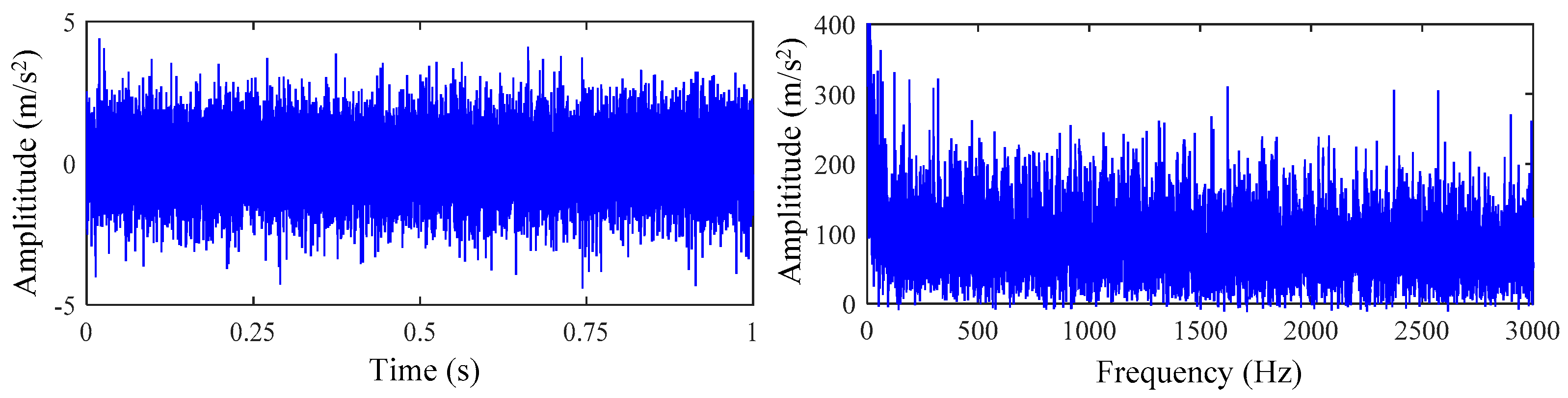
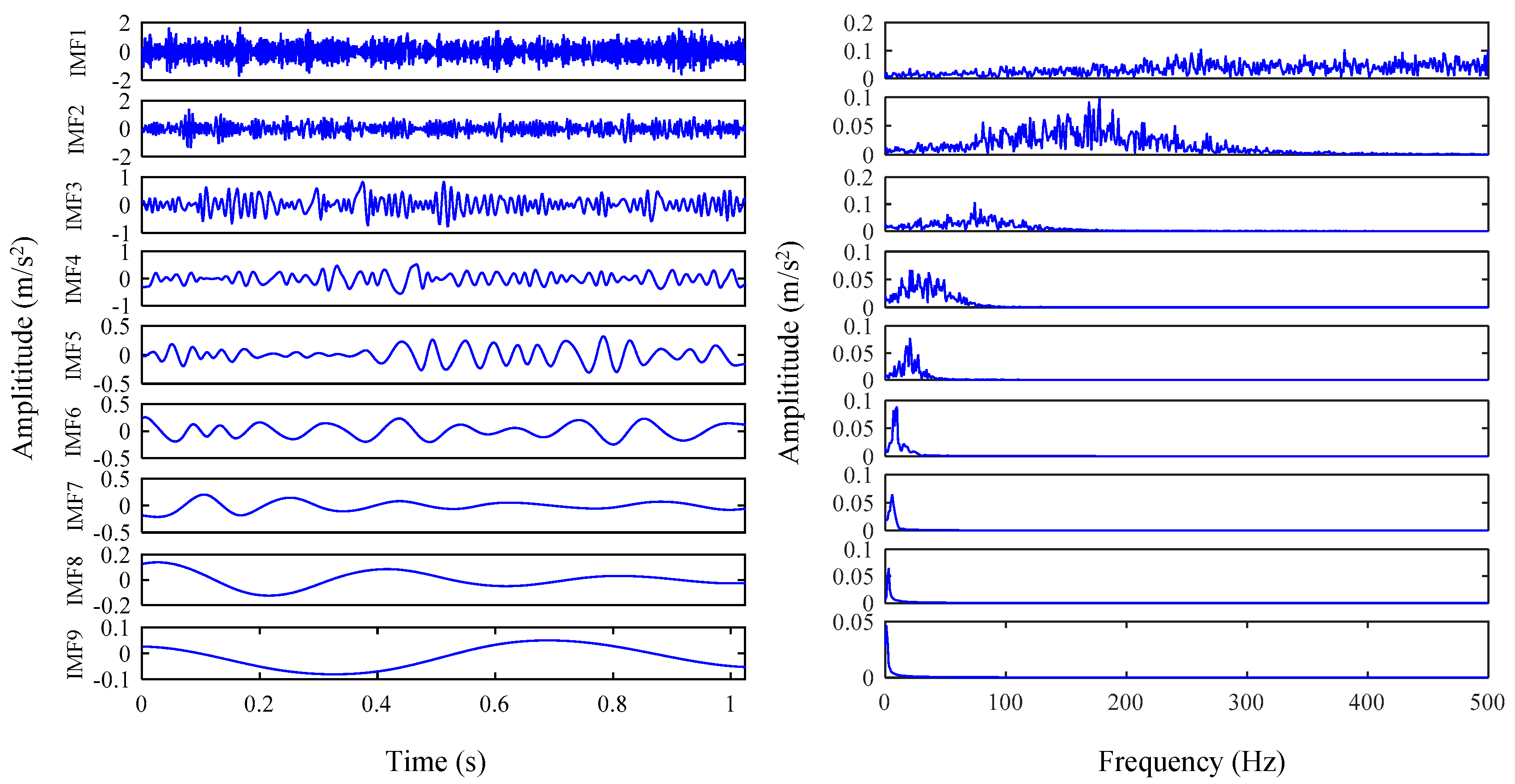
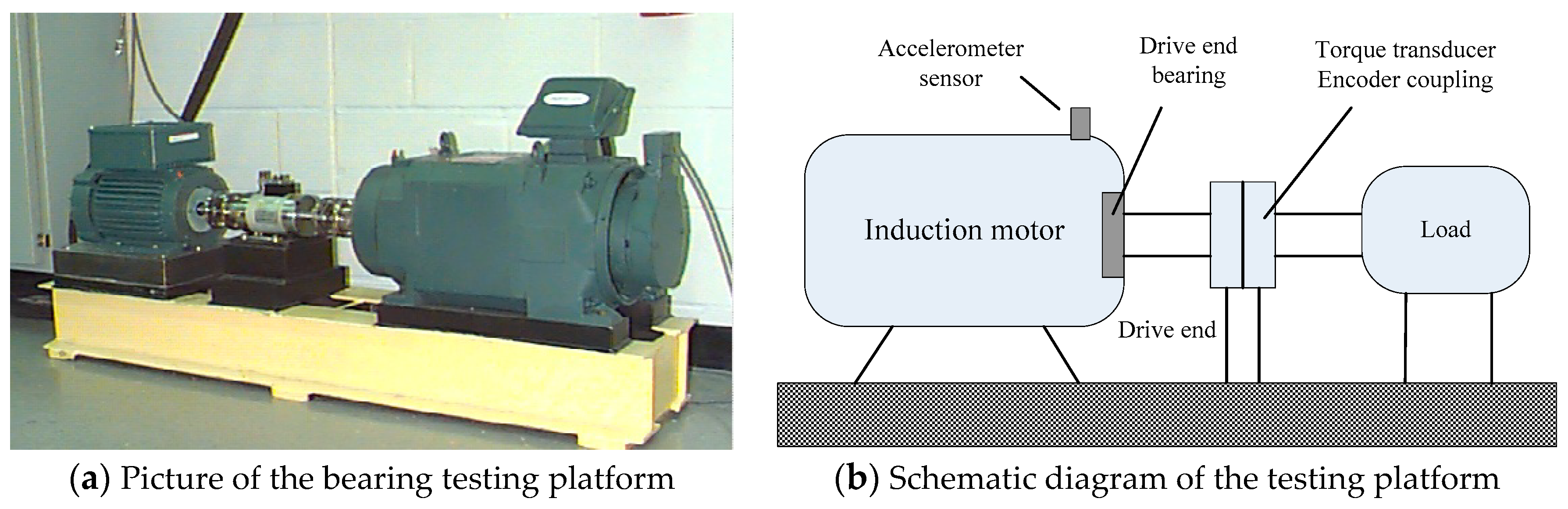
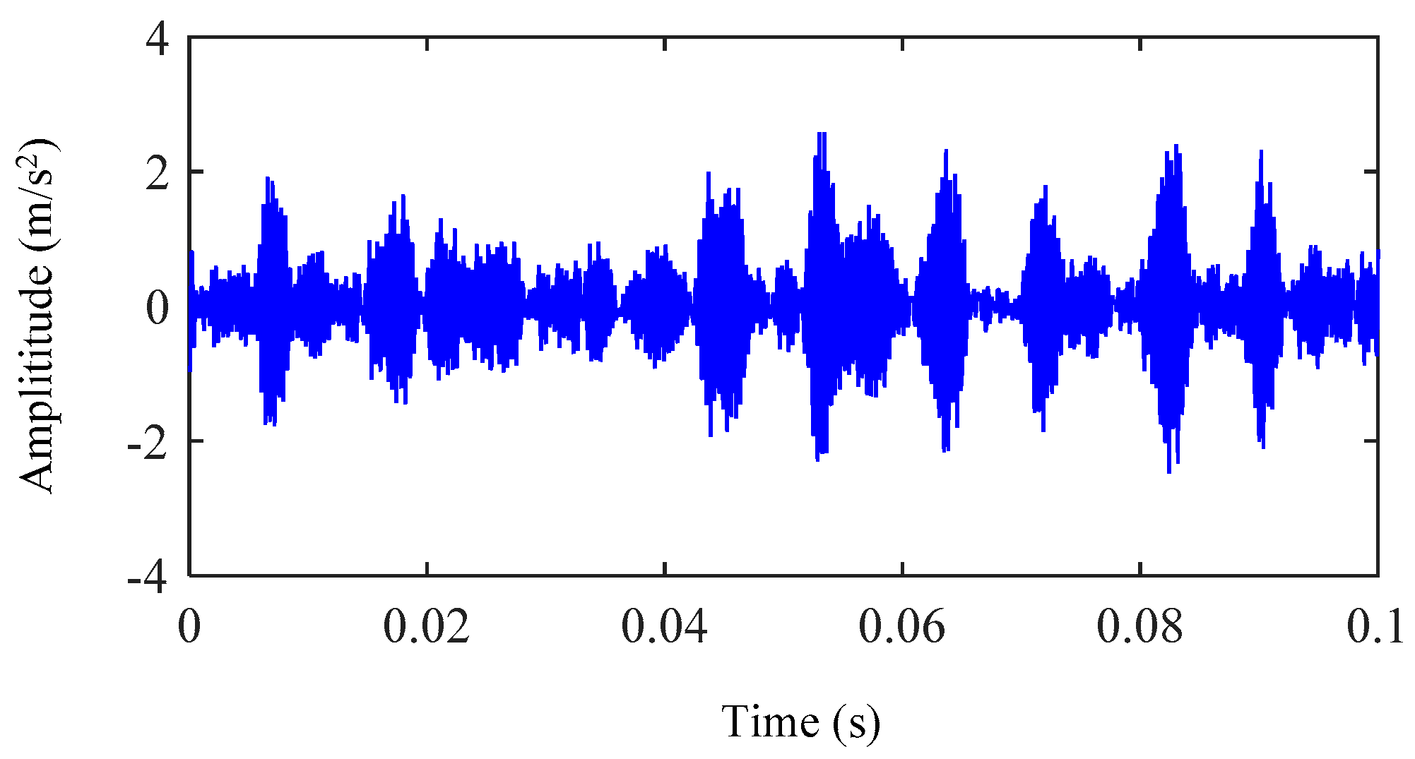
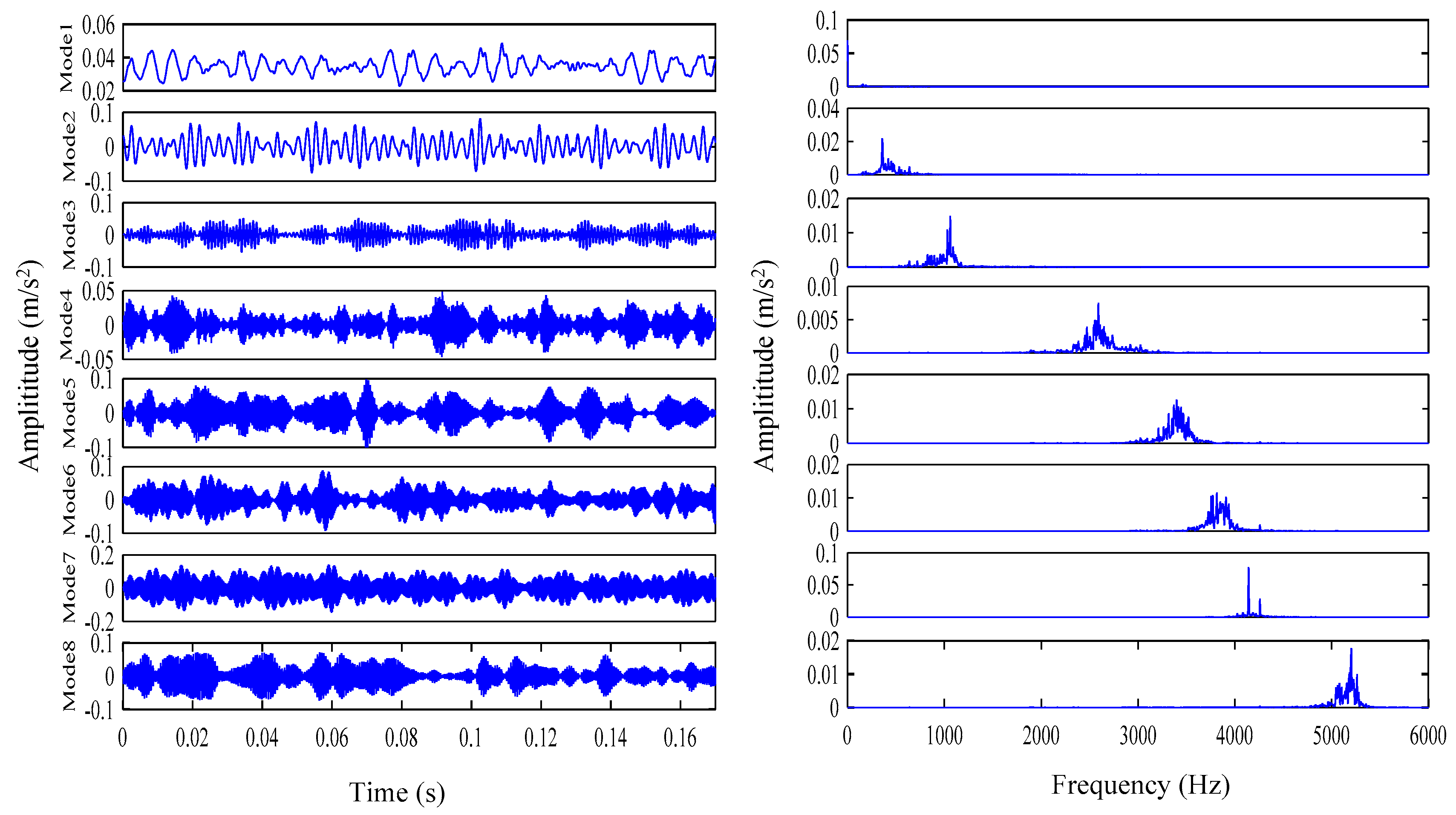
5.2. Actual Vibration Signal Analysis

In order to further verify the IVMD method, the experiment of the actual fault feature extraction is conducted. The bearing vibration data are provided by the Case Western Reserve University (CWRU) Bearing Data Center [40], the rolling bearing failure test rig of CWRU is shown in Figure 16 [40]. The testing platform consisted of a torque transducer/encoder, a dynamometer and a 2 hp, three-phase induction motor. The test bearings support the motor shaft at the drive end. Single point faults are introduced to the test bearings using electro-discharge machining with fault diameters. The dynamometer is utilized to control so that desired torque load levels could be achieved. The deep groove ball bearing with the type of 6205-2RS JEM SKF is employed in the test. The sampling frequency of the vibration data is 12 kHz, the accelerometers are mounted on the drive end of the motor. The vibration signals with the rotational speed of 1797 rpm, the motor load 0 hp and the fault diameters 0.007 inches are chosen to extract the fault feature. The characteristic frequency calculated by geometric parameters is 107.37 Hz.

Figure 17 illustrates representative waveforms of the outer race defects with motor load 0 hp and diameters 0.007in. IMFs from 1 to 9 could be obtained after decomposition by the EMD method. Figure 18 shows the decomposition results and the corresponding frequency spectrum of IMFs. The rolling bearings with partial faults will generate the shock pulse when running. Then the high-frequency vibration is generated, and the amplitude of vibration is modulated by impact force. In order to obtain the fault feature frequency, the bearing vibration signal needs to be demodulated. Because of the complexity of its waveform, it is generally difficult to extract fault information directly from vibration signals. Just as shown in Figure 18, the frequency spectrum of the decomposed IMFs using EMD could not effectively extract the fault feature frequency. Similarly, just as showed in Figure 19, Figure 20, Figure 21 and Figure 22, the frequency spectrums of the decomposed components by using EEMD, CEEMD, VMD and the IVMD could not be effectively identified the fault feature frequency.

Theoretically, the EMD, EEMD, and CEEMD method are equivalent to the filtering process, and the obtained IMFs can be regarded as the component of the vibration signal in a specific frequency band. Therefore, the envelope analysis can be used in the IMF to check the fault feature frequency. The optimal mode component corresponding to the EMD, EEMD, and CEEMD is IMF1, respectively. The envelope spectrum of the optimal component by using EMD, EEMD, and CEEMD is shown in Figure 23, Figure 24 and Figure 25, respectively. It can be seen from Figure 23, Figure 24 and Figure 25 that the impact characteristics associated with faults could be identified, and the feature frequency of fault signals could be extracted. The envelope spectrums of the optimal component by using EMD, EEMD, and CEEMD still had the redundant pseudo components. In addition, the envelope spectrums of the first component processed by the EMD, EEMD, and CEEMD are basically unchanged.

The outer ring defect signal of rolling bearing is decomposed by the VMD method, and six intrinsic mode components could be obtained. Among the six components obtained, the largest efficiency coefficient of the kurtosis corresponding to the mode component 6 is 2.6372. The largest efficiency coefficient of the highest correlation corresponding to the mode component 3 is 0.6781. The smallest efficiency coefficient of the envelope entropy corresponding to the mode component 6 is 3.2370. The envelope spectrum of the optimized reconstruction components is shown as Figure 26. It can be observed in Figure 26 that the spectral amplitude of the envelope spectrum is prominent at the characteristic frequency of 107.37 Hz. At the same time, noise interference still is available in the envelope spectrum of the reconstructed components.

The proposed IVMD method was utilized to analyze the practical bearing vibration signal. The frog of SFLA is only evolved to the first generation to obtain the value of the optimal objective function of 0.9874. The optimal parameter combination obtained by the optimization is [5, 964]. The outer race signal is processed by the IVMD, and the obtained efficacy coefficients corresponding to the decomposed mode components are shown in

Table 2. Efficacy coefficients corresponding to Decomposed Mode components for outer ring defect.

Mode Number	Efficacy Coefficient
	ηK (Kurtosis)	ηC (Correlation Degree)	ηE (Envelope Entropy)
1	3.5669	0.1121	3.2413
2	2.6746	0.4765	3.2577
3	3.1393	0.7161	3.2524
4	3.1648	0.6993	3.2296
5	3.8560	0.2220	3.2358

. Among the obtained eight components, the largest efficiency coefficient of the kurtosis corresponding to the mode component 5 is 3.8560. The largest efficiency coefficient of the highest correlation corresponding to the mode component 3 is 0.7161. The smallest efficiency coefficient of the envelope entropy corresponding to the mode component 4 is 3.2296. The envelope spectrum of reconstruction components is shown in Figure 27. It could be seen from Figure 27 that the spectral amplitude of the envelope spectrum was prominent at the characteristic frequency 80Hz, and the clear peak spectra is also observed at the double frequency of the fault frequencies. Compared with the VMD method without optimization, the fault frequency extracted by the IVMD method is more prominent and the noise is also suppressed.

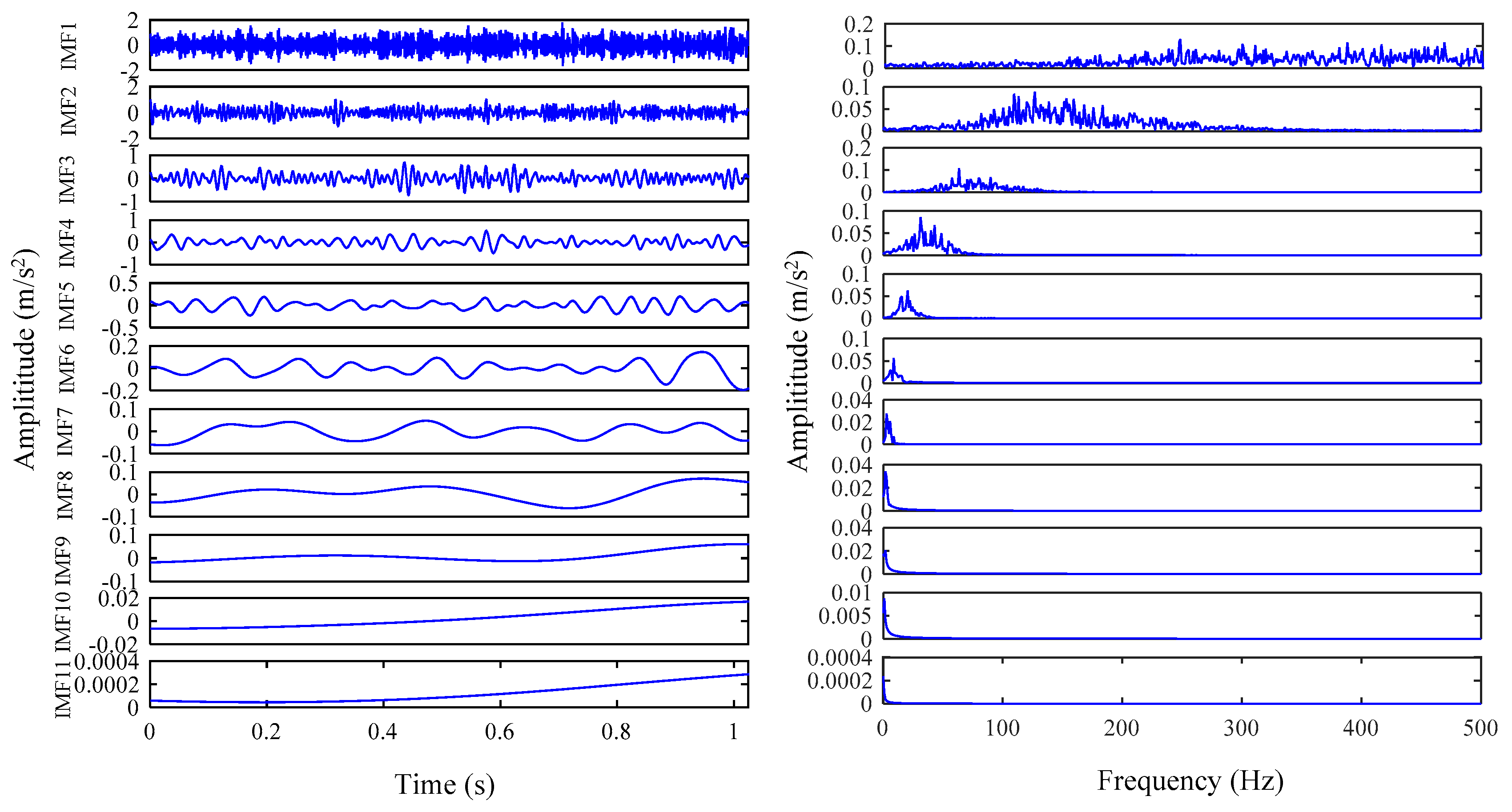
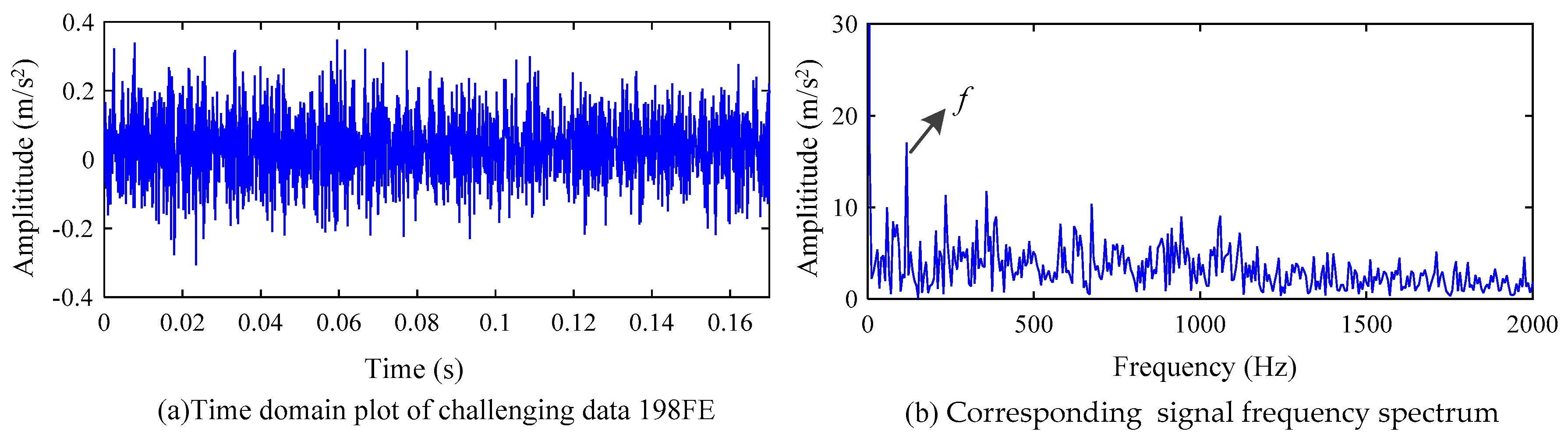
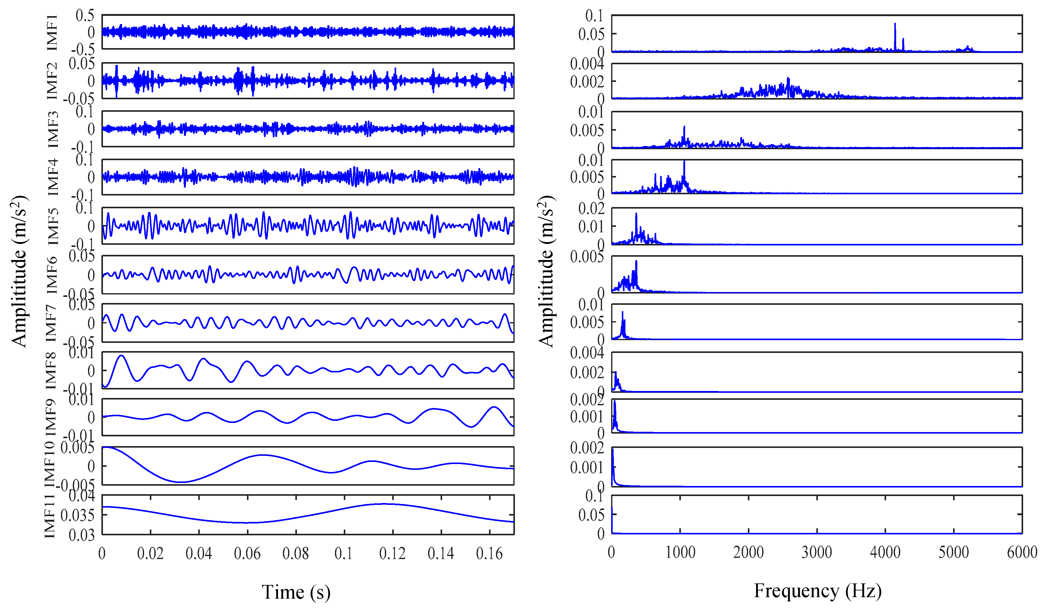
5.3. Challenging Data Analysis

However, the experimental data from CWRU Bearing Data Center have their own unique characteristics. A comprehensive study of CWRU data has been provided in the document, this study provides a benchmark analysis by using three established bearing diagnostic techniques [41,42]. It was noted that the data records ranged from very easily diagnosable (using simple envelope analysis of the raw signal) to not diagnosable with any of the applied methods. In the literature, these data that could not be diagnosed using three given methods were called challenging data. To further verify the applicability of the proposed diagnostic algorithms, the challenging data 198FE is used for robustness testing, which was listed in the literature [41,42]. The rotational speed of challenging data 198FE is 1772 rpm, the motor load is 1 hp and the fault diameter is 0.014 inches. The feature frequency of the outer race defect is 105.87 Hz. The time-domain plot and the envelope spectrum of challenging data 198FE are shown in Figure 28.

It can be seen from Figure 28 that the challenging signal was submerged in the strong background noise in the time domain plot. The feature frequency of the challenging data could be found from the envelope spectrum, but the serious noise interference still existed in the envelope spectrum.

The challenging data is decomposed by CEEMD, VMD, and the proposed IVMD method, respectively. The decomposition results and corresponding frequency spectrums were shown in Figure 29, Figure 30 and Figure 31. It can be seen from Figure 29, Figure 30 and Figure 31 that the feature frequency could not be effectively distinguished.

The envelope spectrum of the optimal component of challenging signal by using CEEMD is shown in Figure 32. Among five components decomposed by the VMD method in Figure 30, according to the multi-objective evaluation function, the largest efficiency coefficient of the kurtosis corresponding to the mode component 3 is 3.2639. The largest efficiency coefficient of the highest correlation corresponding to the mode component 4 is 0.7357. The smallest efficiency coefficient of the envelope entropy corresponding to the mode component 3 is 3.2436. The envelope spectrum of the reconstruction component by the mode components 3 and 4 is shown in Figure 33. It can be observed in Figure 32 and Figure 33 that the impact characteristics associated with the faults could be identified, the feature frequency of the challenging signal could be extracted. However, envelope spectrums of the optimal component by using CEEMD and VMD still had the redundant pseudo components. Compared with Figure 32 and Figure 33, the envelope spectrum of the optimal component obtained by the VMD method is better than that by the CEEMD method in the noise reduction, and the fault characteristic frequency is more prominent.

The IVMD method is applied to analyze the challenging signal. The relationship between the value of the objective function and the number of evolutionary iterations is shown in Figure 34. It can be seen from Figure 34 that the frog of SFLA is only evolved to the second generation. The value of the optimal objective function is 0.6054. The optimal parameter combination obtained by the optimization is [8, 1137]. The challenging data are processed by the IVMD, the obtained efficacy coefficients corresponding to the decomposed mode components are as shown in

Table 3. Efficacy coefficients corresponding to Decomposed Mode components to the challenging signal.

Mode Number	Efficacy Coefficient
	ηK (Kurtosis)	ηC (Correlation Degree)	ηE (Envelope Entropy)
1	2.4683	0. 0910	3.3077
2	2.4792	0.1832	3.2730
3	2.9384	0.0134	3.2527
4	3.6555	0.0885	3.2390
5	2.7657	0.2204	3.2524
6	2.7522	0.2287	3.2509
7	1.8823	0.6227	3.2961
8	2.8763	0.2941	3.2673

. Among the obtained eight components, the largest efficiency coefficient corresponding to the mode component 4 for the kurtosis is 3.6555. The largest efficiency coefficient corresponding to the mode component 7 is 0.6227 for the highest correlation. The smallest efficiency coefficient of the envelope entropy corresponding to the mode component 4 is 3.2390. The envelope spectrum of optimized reconstruction components is shown as Figure 35. It can be seen from Figure 35 that the spectral amplitude of the envelope spectrum is prominent at the characteristic frequency of 105.87 Hz, which means that the IVMD can correctly decompose the challenging signal and accurately extract the feature frequency of the challenging data. Compared with the VMD method without optimization, the fault frequency extracted by the proposed method is more prominent and the noise is also effectively suppressed.

6. Conclusions

The completely non-recursive signal modal variational nature of the VMD method makes it more advantageous than the EMD and its extension methods in terms of robustness against noise, overcoming end effects and mode aliasing. However, the decomposition accuracy of VMD method is affected by the choice of mode number K and bandwidth control parameter α. The IVMD in this paper was developed to achieve the accurate decomposition of fault signal and adaptive control of influence parameters. The shuffled frog leaping algorithm was used to implement the optimization the influence parameters. The multi-objective evaluation function was constructed for the selection of the optimal mode component and the calculation of fitness value, which is based on the envelope entropy, the kurtosis, and the correlation coefficients. The envelope spectrum technique was used to analyze the optimal mode component. According to the characteristics of the vibration signal, we built the simulation signal to verify the feasibility and effectiveness of the signal, and also used the vibration data of Case Western Reserve University Bearing Data Center to verify the proposed method.

A series of experiments were conducted, and the results proved the effectiveness of the proposed fault feature extraction method for the rolling element bearing fault diagnosis. The IVMD method could achieve the optimal combination of influencing parameters, improve the accuracy of decomposition, effectively extract the fault feature and eliminate the noise interference. The results also show that the fault feature extraction performance of the improved VMD method is better than the original VMD algorithm, and the improved VMD method achieves a higher fault diagnosis accuracy than the original VMD algorithm, EMD, EEMD and CEEMD.

The operating condition of rolling bearings is uncertain, and this uncertainty makes the distribution differences for the data of different operating conditions, so the proposed methods need to be further improved. In the time–frequency domain, combining the improved method with transfer learning, and studying the robustness of the improved method for extracting fault features under different working conditions and different types of faults is the work of future research.

References

1. Liu, R.; Yang, B.; Zio, E.; Chen, X. Artificial intelligence for fault diagnosis of rotating machinery: A review. Mech. Syst. Signal Process. 2018, 108, 33–47. [Google Scholar] [CrossRef]
2. Jiang, H.; Li, X.; Shao, H.; Zhao, K. Intelligent fault diagnosis of rolling bearings using an improved deep recurrent neural network. Meas. Sci. Technol. 2018, 29, 065107. [Google Scholar] [CrossRef]
3. Xiong, S.; Zhou, H.; He, S.; Zhang, L.; Xia, Q.; Xuan, J.; Shi, T. A novel end-to-end fault diagnosis approach for rolling bearings by integrating wavelet packet transform into convolutional neural network structures. Sensors 2020, 20, 4965. [Google Scholar] [CrossRef] [PubMed]
4. Yan, X.; Liu, Y.; Jia, M.; Zhu, Y. A multi-stage hybrid fault diagnosis approach for rolling element bearing under various working conditions. IEEE Access 2019, 7, 138426–138441. [Google Scholar] [CrossRef]
5. Chen, F.; Cheng, M.; Tang, B.; Xiao, W.; Chen, B.; Shi, X. A novel optimized multi-kernel relevance vector machine with selected sensitive features and its application in early fault diagnosis for rolling bearings. Measurement 2020, 156, 107583. [Google Scholar] [CrossRef]
6. Zhao, X.; Jia, M. Fault diagnosis of rolling bearing based on feature reduction with global-local margin Fisher analysis. Neurocomputing 2018, 315, 447–464. [Google Scholar] [CrossRef]
7. Chaabi, L.; Lemzadmi, A.; Djebala, A.; Bouhalais, M.L.; Ouelaa, N. Fault diagnosis of rolling bearings in non-stationary running conditions using improved CEEMDAN and multivariate denoising based on wavelet and principal component analyses. Int. J. Adv. Manuf. Technol. 2020, 107, 3859–3873. [Google Scholar] [CrossRef]
8. Randall, R.B.; Antoni, J. Rolling element bearing diagnostics—A tutorial. Mech. Syst. Signal Process. 2011, 25, 485–520. [Google Scholar] [CrossRef]
9. Dong, G.; Chen, J. Noise resistant time frequency analysis and application in fault diagnosis of rolling element bearings. Mech. Syst. Signal Process. 2012, 33, 212–236. [Google Scholar] [CrossRef]
10. Guo, J.; Zhen, D.; Li, H.; Shi, Z.; Gu, F.; Ball, A.D. Fault feature extraction for rolling element bearing diagnosis based on a multi-stage noise reduction method. Measurement 2019, 139, 226–235. [Google Scholar] [CrossRef] [Green Version]
11. Wang, D.; Zhao, Y.; Yi, C.; Tsui, K.L.; Lin, J. Sparsity guided empirical wavelet transform for fault diagnosis of rolling element bearings. Mech. Syst. Signal Process. 2018, 101, 292–308. [Google Scholar] [CrossRef]
12. Singh, J.; Darpe, A.K.; Singh, S.P. Rolling element bearing fault diagnosis based on over-complete rational dilation wavelet transform and auto-correlation of analytic energy operator. Mech. Syst. Signal Process. 2018, 100, 662–693. [Google Scholar] [CrossRef]
13. Wang, C.; Gan, M. Fault feature extraction of rolling element bearings based on wavelet packet transform and sparse representation theory. J. Intell. Manuf. 2018, 29, 937–951. [Google Scholar] [CrossRef]
14. Tong, Q.; Cao, J.; Han, B.; Zhang, X.; Nie, Z.; Wang, J.; Lin, Y.; Zhang, W. A fault diagnosis approach for rolling element bearings based on RSGWPT-LCD bilayer screening and extreme learning machine. IEEE Access 2017, 5, 5515–5530. [Google Scholar] [CrossRef]
15. Huang, W.; Kong, F.; Zhao, X. Spur bevel gearbox fault diagnosis using wavelet packet transform and rough set theory. J. Intell. Manuf. 2018, 29, 1257–1271. [Google Scholar] [CrossRef]
16. Huang, N.E.; Shen, Z.; Long, S.R.; Wu, M.C.; Shih, H.H.; Zheng, Q.; Yen, N.C.; Tung, N.C.; Liu, H.H. The empirical mode decomposition and the Hilbert spectrum for nonlinear and non-stationary time series analysis. Proc. R Soc. Lond. Ser. A Math. Phys. Eng. Sci. 1998, 454, 903–995. [Google Scholar] [CrossRef]
17. Xu, Y.; Cai, Z.; Ding, K. An enhanced bearing fault diagnosis method based on TVF-EMD and a high-order energy operator. Meas. Sci. Technol. 2018, 29, 095108. [Google Scholar] [CrossRef]
18. Wang, J.; Du, G.; Zhu, Z.; Shen, C.; He, Q. Fault diagnosis of rotating machines based on the EMD manifold. Mech. Syst. Signal Process. 2020, 135, 106443. [Google Scholar] [CrossRef]
19. Abdelkader, R.; Kaddour, A.; Derouiche, Z. Enhancement of rolling bearing fault diagnosis based on improvement of empirical mode decomposition denoising method. Int. J. Adv. Manuf. Technol. 2018, 97, 3099–3117. [Google Scholar] [CrossRef]
20. Ye, X.; Hu, Y.; Shen, J.; Feng, R.; Zhai, G. An improved empirical mode decomposition based on adaptive weighted rational quartic spline for rolling bearing fault diagnosis. IEEE Access 2020, 8, 123813–123827. [Google Scholar] [CrossRef]
21. Fan, H.; Shao, S.; Zhang, X.; Wan, X.; Cao, X.; Ma, H. Intelligent fault diagnosis of rolling bearing using FCM clustering of EMD-PWVD vibration images. IEEE Access 2020, 8, 145194–145206. [Google Scholar] [CrossRef]
22. Mohanty, S.; Gupta, K.K.; Raju, K.S. Hurst based vibro-acoustic feature extraction of bearing using EMD and VMD. Measurement 2018, 117, 200–220. [Google Scholar] [CrossRef]
23. Niu, Y.; Fei, J.; Li, Y.; Wu, D. A novel fault diagnosis method based on EMD, cyclostationary, SK and TPTSR. J. Mech. Sci. Technol. 2020, 34, 1925–1935. [Google Scholar] [CrossRef]
24. Han, D.; Zhao, N.; Shi, P. Gear fault feature extraction and diagnosis method under different load excitation based on EMD, PSO-SVM and fractal box dimension. J. Mech. Sci. Technol. 2019, 33, 487–494. [Google Scholar] [CrossRef]
25. Wu, Z.; Huang, N.E. Ensemble empirical mode decomposition: A noise-assisted data analysis method. Adv. Adapt. Data Anal. 2009, 1, 1–41. [Google Scholar] [CrossRef]
26. Jiang, F.; Zhu, Z.; Li, W.; Ren, Y.; Zhou, G.; Chang, Y. A fusion feature extraction method using EEMD and correlation coefficient analysis for bearing fault diagnosis. Appl. Sci. 2018, 8, 1621. [Google Scholar] [CrossRef] [Green Version]
27. Han, T.; Liu, Q.; Zhang, L.; Tan, A.C. Fault feature extraction of low speed roller bearing based on Teager energy operator and CEEMD. Measurement 2019, 138, 400–408. [Google Scholar] [CrossRef]
28. Liu, F.; Gao, J.; Liu, H. The feature extraction and diagnosis of rolling bearing based on CEEMD and LDWPSO-PNN. IEEE Access 2020, 8, 19810–19819. [Google Scholar] [CrossRef]
29. Dragomiretskiy, K.; Zosso, D. Variational mode decomposition. IEEE Trans. Signal Process. 2013, 62, 531–544. [Google Scholar] [CrossRef]
30. Wang, Y.; Markert, R.; Xiang, J.; Zheng, W. Research on variational mode decomposition and its application in detecting rub-impact fault of the rotor system. Mech. Syst. Signal Process. 2015, 60, 243–251. [Google Scholar] [CrossRef]
31. Zhao, H.; Liu, H.; Xu, J.; Guo, C.; Deng, W. Research on a fault diagnosis method of rolling bearings using variation mode decomposition and deep belief network. J. Mech. Sci. Technol. 2019, 33, 4165–4172. [Google Scholar] [CrossRef]
32. Eusuff, M.; Lansey, K.; Pasha, F. Shuffled frog-leaping algorithm: A memetic meta-heuristic for discrete optimization. Eng. Optimiz. 2006, 38, 129–154. [Google Scholar] [CrossRef]
33. Eusuff, M.M.; Lansey, K.E. Optimization of water distribution network design using the shuffled frog leaping algorithm. J. Water. Res. Plan. Manag. 2003, 129, 210–225. [Google Scholar] [CrossRef]
34. Pérez-Delgado, M.L. Color image quantization using the shuffled-frog leaping algorithm. Eng. Appl. Artif. Intel. 2019, 79, 142–158. [Google Scholar] [CrossRef]
35. Venkatesan, T.; Sanavullah, M.Y. SFLA approach to solve PBUC problem with emission limitation. Int. J. Elec. Power 2013, 46, 1–9. [Google Scholar] [CrossRef]
36. Sun, J.; Xiao, Q.; Wen, J.; Wang, F. Natural gas pipeline small leakage feature extraction and recognition based on LMD envelope spectrum entropy and SVM. Measurement 2014, 55, 434–443. [Google Scholar] [CrossRef]
37. Sawalhi, N.; Randall, R.; Endo, H. The enhancement of fault detection and diagnosis in rolling element bearings using minimum entropy deconvolution combined with spectral kurtosis. Mech. Syst. Signal Process. 2007, 21, 2616–2633. [Google Scholar] [CrossRef]
38. Wang, S.; Huang, W.; Zhu, Z.K. Transient modeling and parameter identification based on wavelet and correlation filtering for rotating machine fault diagnosis. Mech. Syst. Signal Process. 2011, 25, 1299–1320. [Google Scholar] [CrossRef]
39. Chen, Q.; Wang, C.; Wen, P.; Wang, M.; Zhao, J. Comprehensive performance evaluation of low-carbon modified asphalt based on efficacy coefficient method. J. Clean. Prod. 2018, 203, 633–644. [Google Scholar] [CrossRef]
40. Case Western Reserve University Bearing Data Center. Seeded Fault Test Data. 2012. Available online: https://csegroups.case.edu/bearingdatacenter/home (accessed on 18 January 2019).
41. Li, X.; Zhang, W.; Ding, Q. Cross-domain fault diagnosis of rolling element bearings using deep generative neural networks. IEEE Trans. Ind. Electron. 2018, 66, 5525–5534. [Google Scholar] [CrossRef]
42. Smith, W.A.; Randall, R.B. Rolling element bearing diagnostics using the Case Western Reserve University data: A benchmark study. Mech. Syst. Signal Process. 2015, 64, 100–131. [Google Scholar] [CrossRef]
Figure 1. Flowchart of the parameter optimization by using the Shuffled Frog Leap Algorithm (SFLA).
Energies 14 01079 g001
Figure 2. Flowchart of the fault feature extraction by using parameters-optimized Variational mode decomposition (VMD).
Energies 14 01079 g002
Figure 3. Time-domain plot of simulated signal and corresponding frequency spectrum.
Energies 14 01079 g003
Figure 4. Decomposition results and corresponding frequency spectrum of intrinsic mode functions (IMFs) with Empirical Mode Decomposition (EMD).
Energies 14 01079 g004
Figure 5. Decomposition results and corresponding frequency spectrum of IMFs with Ensemble EMD (EEMD).
Energies 14 01079 g005
Figure 6. Decomposition results and corresponding frequency spectrum of IMFs with complementary ensemble empirical mode decomposition (CEEMD).
Energies 14 01079 g006
Figure 7. Decomposition results and corresponding frequency spectrum of modes with VMD.
Energies 14 01079 g007
Figure 8. Decomposition results and corresponding frequency spectrum of modes by using improved variational mode decomposition (IVMD).
Energies 14 01079 g008
Figure 9. Residues of added white noises derived by EEMD and CEEMD.
Energies 14 01079 g009
Figure 10. Envelope spectrum of optimal component by using EMD.
Energies 14 01079 g010
Figure 11. Envelope spectrum of optimal component by using EEMD.
Energies 14 01079 g011
Figure 12. Envelope spectrum of optimal component by using CEEMD.
Energies 14 01079 g012
Figure 13. Envelope spectrum of optimal component by using VMD.
Energies 14 01079 g013
Figure 14. Changing curve of between the value of the objective function and the iteration number.
Energies 14 01079 g014
Figure 15. Envelope spectrum of optimal component by using IVMD.
Energies 14 01079 g015
Figure 16. Rolling bearing failure test rig of Case Western Reserve University (CWRU) [40].
Energies 14 01079 g016
Figure 17. Time domain plot of the signal with outer race defect.
Energies 14 01079 g017
Figure 18. Decomposition results and corresponding frequency spectrum of the IMFs for outer ring defect using EMD.
Energies 14 01079 g018
Figure 19. Decomposition results and corresponding frequency spectrum of IMFs for outer ring defect with EEMD.
Energies 14 01079 g019
Figure 20. Decomposition results and corresponding frequency spectrum of IMFs for outer ring defect with CEEMD.
Energies 14 01079 g020
Figure 21. Decomposition results and corresponding frequency spectrum of modes for outer ring defect with VMD.
Energies 14 01079 g021
Figure 22. Decomposition results and corresponding frequency spectrum of modes by IVMD.
Energies 14 01079 g022
Figure 23. The envelope spectrum of the optimal component for outer ring defect by using EMD.
Energies 14 01079 g023
Figure 24. The envelope spectrum of the optimal component for outer ring defect by using EEMD.
Energies 14 01079 g024
Figure 25. The envelope spectrum of the optimal component for outer ring defect by using CEEMD.
Energies 14 01079 g025
Figure 26. The envelope spectrum of the optimal component for outer ring defect by using VMD.
Energies 14 01079 g026
Figure 27. The envelope spectrum of the optimal component by using IVMD.
Energies 14 01079 g027
Figure 28. Time domain plot of challenging data 198FE and envelope spectrum.
Energies 14 01079 g028
Figure 29. Decomposition results and corresponding frequency spectrum of the IMFs for challenging signal with CEEMD.
Energies 14 01079 g029
Figure 30. Decomposition results and corresponding frequency spectrum of the IMFs for challenging signal with VMD.
Energies 14 01079 g030
Figure 31. Decomposition results and corresponding frequency spectrum of the IMFs for challenging signal with IVMD.
Energies 14 01079 g031
Figure 32. Envelope spectrum of optimal component of challenging signal by using CEEMD.
Energies 14 01079 g032
Figure 33. Envelope spectrum of optimal component of challenging signal by using VMD.
Energies 14 01079 g033
Figure 34. Variation curve of between the objective function and the number of evolutionary iterations for the challenging signal.
Energies 14 01079 g034
Figure 35. Envelope spectrum of optimal component of challenging signal by using IVMD.
Energies 14 01079 g035