Load Frequency Regulator in Interconnected Power System Using Second-Order Sliding Mode Control Combined with State Estimator

Abstract

In multi-area interconnected power systems (MAIPS), the measurement of all system states is difficult due to the lack of a sensor or the fact that it is expensive to measure. In order to solve this limitation, a new load frequency controller based on the second-order sliding mode is designed for MAIPS where the estimated state variable is used fully in the sliding surface and controller. Firstly, a model of MAIPS integrated with disturbance is introduced. Secondly, an observer has been designed and used to estimate the unmeasured variables with disturbance. Thirdly, a new second-order sliding mode control (SOSMC) law is used to reduce the chattering in the system dynamics where slide surface and sliding mode controller are designed based on system states observer. The stability of the whole system is guaranteed via the Lyapunov theory. Even though state variables are not measured, the experimental simulation results show that the frequency remains in the nominal range under load disturbances, matched and mismatched uncertainties of the MAIPS. A comparison to other controllers illustrates the superiority of the highlighted controller designed in this paper.

1. Introduction

In modern multi-area power systems (MAPS), where the power plants are geographically distributed, maintaining the tie-power flow and frequency are the central aspects of the MAPS. At sudden change in the net load, frequency and tie-schedule power deviate from nominal. Therefore, it is essential to preserve the quality of the generated power in the power plant through designing a load frequency control (LFC) [1,2,3,4,5,6]. The general function of the LFC is to maintain the balance between the new net-load demand and the generated power by regulating the tie-line and frequency power flow in MAPS.

In general, power plants are connected together via tie-lines. Maintaining scheduled power flows between interconnected large systems is very crucial. Moreover, keeping the frequencies of each area in a nominal range where the plant model exhibits the following drawbacks: random load change, and mismatched uncertainties. These made the LFC design more complex [7]. Thus, two approaches are used for LFC in the interconnected power network: a centralized and decentralized LFC scheme where the second scheme is preferable as the controller feed-in by the regional information [8,9,10].

There are a lot of control methods that have been designed for LFC, and the significant research papers were proposed for LFC as summarized in [11]. Proportional integral (PI) is the first control method studied in the field of LFC, where the mismatched parameters were neglected. It follows that the PI tuned once for specific operating conditions, hence the PI controller failed under variable operating points [12]. In recent years, some advanced control methods have also been developed. Some intelligent control schemes such as particle swarm optimization, fuzzy logic, artificial neural network and genetic algorithm have been proposed for LFC in MAPS [13,14,15,16,17]. In addition, the optimal control scheme with Proportional integral derivative (PID), particularly the particle swarm optimization (PSO) algorithm, was implemented for tuning PID-based LFC [18]. However, the above-proposed controllers consider the mismatched uncertainty of the power systems [19].

Robust control scheme such as variable structure control (VSC) is used to control power frequency. VSC is robust against various power system problems. VSC for LFC for MAPS is presented in [20]. Among the VSC control methods, sliding mode control (SMC) has been greatly used by control engineers. The SMC method is discussed in [21]. The SMC control strategy provides robust performance and fast response. Discrete and continuous time SMC for LFC are examined for power systems [22,23], respectively. A decentralized SMC with an integral sliding surface is studied and presented in [24]. In the literature, the SMC discussed acts on a first-order time derivative. The first-order SMC combination with state observer is provided for LFC in MAPS which is suffered from chattering phenomenon [25]. The second-order sliding mode control (SOSMC) has been proposed to handle this problem [26]. The system state variables were assumed to be measured [20,21,22,23,24,25,26]. In contrast, some state variables of the real power system are difficult to measure. The direct measurements with sensors in some cases are difficult or expensive for the measurement. In order to solve the above problem, the state observer has been widely explored for industrial application such as the Luenberger observer [27], unscented Kalman filter [28] and extended observer [29] where the system performance is also affected by matched uncertainty. The state estimator for LFC of MAPS is employed and presented in [29]. With the aim of improving the system performance, first-order SMC based on an observer has been used to observe the load disturbance of the power network given in [30,31]. Also, SOSMC combined with a state estimator has been used to observe the disturbance of the MAPS to improve the system performance with making it free of chattering [32,33]. These controllers above were designed to observe the load change and keep the frequency at nominal if all the system state variables are measured. However, this cannot guarantee for the practical application of these above controllers where some state variables of MAPS are not measurable or difficult to measure. Therefore, this motivates the design of LFC based on a new SMC where the state observer is used fully in the sliding surface and a decentralized second-order sliding mode controller (SOSMCr) is used to solve the above the problems. The major contributions of the paper are as below:

• The integral sliding surface (ISS) and the decentralized controller are designed based on the estimated system state variables (SSV) so that we do not need to measure the power SSV to achieve LFC. Therefore, the limitation of measuring the power system state variables to achieve LFC in [32,33] has been solved.
• A new LMI technique is proposed to ensure the stability of MAPS via the Lyapunov theory.
• SOSMC combined with state estimator is designed to improve the system performance due to a decrease in chattering in the control input.
• The simulation results indicate the proposed approach has a better performance in terms of settling time and under/overshoots. Thus, this provides evidence of the new controller application for large MAPS.

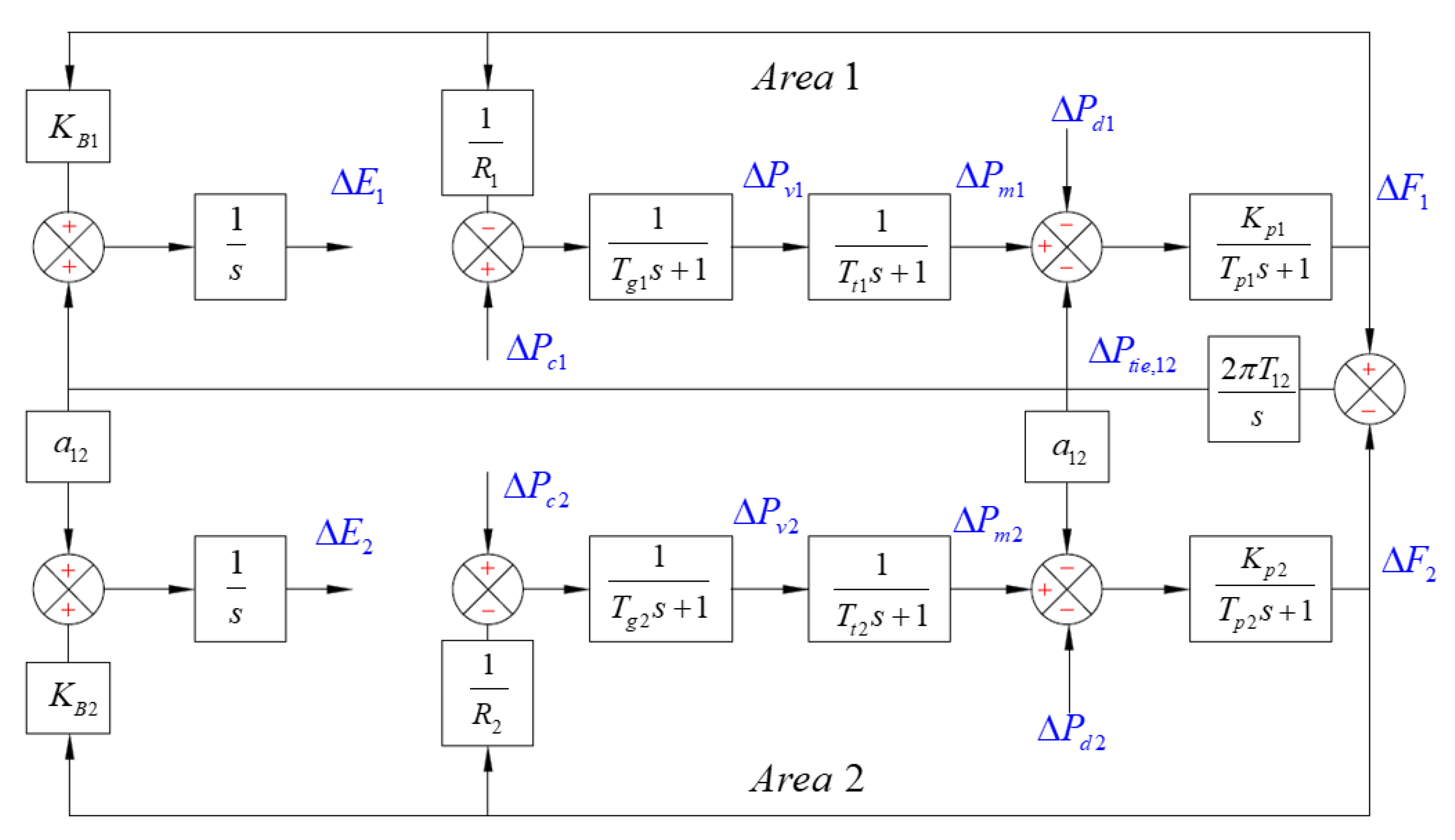
2. Model of Two-Area Power System (TAPS) in State Space Form

In this section, we introduce the linear dynamic equations for TAPS. A representative diagram of a decentralized LFC for the system is presented in Figure 1. Both areas have their proposed local controller which will be designed in the following sections. The interconnected power line and frequency are kept constant by the proposed local controller. In general, the frequency regulator scheme consists of two feedback loops, mainly the primary LFC loop (inner loop) and secondary LFC loop (outer loop). The inner loop consists of governor droop speed. The outer loop consists of the proposed controller.

The SSV denoted in Figure 1 describes the dynamics of the TAPS.

Using the above system model, the following differential equations are obtained

$$\Delta {\dot{f}}_1=-\frac{1}{T_{p1}}\Delta f_1+\frac{K_{p1}}{T_{p1}}\Delta P_{m1}-\frac{K_{p1}}{T_{p1}}\Delta P_{tie1,2}-\frac{K_{p1}}{T_{p1}}\Delta P_{d1}$$

(1)

$$\Delta {\dot{P}}_{m1}=-\frac{1}{T_{t1}}\Delta P_{m1}+\frac{1}{T_{t1}}\Delta P_{v1}$$

(2)

$$\Delta {\dot{P}}_{v1}=-\frac{1}{R_1{T}_{g1}}\Delta f_1-\frac{1}{T_{g1}}\Delta P_{v1}+\frac{1}{T_{g1}}\Delta P_{c1}$$

(3)

$$\Delta {\dot{f}}_2=-\frac{1}{T_{p2}}\Delta f_2+\frac{K_{p2}}{T_{p2}}\Delta P_{m2}-\frac{a_{12}{K}_{p2}}{T_{p2}}\Delta P_{tie1,2}-\frac{K_{p2}}{T_{p2}}\Delta P_{d2}$$

(4)

$$\Delta {\dot{P}}_{m2}=-\frac{1}{T_{t2}}\Delta P_{m2}+\frac{1}{T_{t2}}\Delta P_{v2}$$

(5)

$$\Delta {\dot{P}}_{v2}=-\frac{1}{R_2{T}_{g2}}\Delta f_2-\frac{1}{T_{g2}}\Delta P_{v2}+\frac{1}{T_{g2}}\Delta P_{c2}$$

(6)

$$\Delta P_{tie1,2}=2\pi T_{12}\Delta f_1-2\pi T_{12}\Delta f_2$$

(7)

$$\Delta {\dot{E}}_1=K_B{}_1\Delta f_1+\Delta P_{tie1,2}$$

(8)

$$\Delta {\dot{E}}_2=K_{B2}\Delta f_2+a_{12}\Delta P_{tie1,2}$$

(9)

where $\Delta f_1$ and $\Delta f_2$ are the frequency deviations of the first and second areas, $\Delta P_{m1}$ and $\Delta P_{m2}$ are the generator mechanical output deviations of the first and second areas, $\Delta P_{v1}$ and $\Delta P_{v2}$ are the valve position deviations of first and second areas, $\Delta E_1$ and $\Delta E_2$ are the area control errors of first and second areas, $\Delta P_{tie1,2}$ is the tie-line active power deviation between the first and second areas. $K_{p1}$ and $K_{p2}$ are operations of the system power of the first and second areas, $T_{p1}$ and $T_{p2}$ are time constants of the power system of the first and second areas, $T_{t1}$ and $T_{t2}$ are turbine time constants of the first and second areas, $T_{g1}$ and $T_{g2}$ are governor time constants of steam of the first and second areas, $R_1$ and $R_2$ are speed drops of the first and second areas, $K_B{}_1$ and $K_B{}_2$ are frequency bias factors of the first and second areas, $T_{12}$ is the tie-line reactance and synchronizing coefficient between the first and second areas, and $a_{12}$ is the control area capacity ratio.

The system dynamic Equations (1)–(9) are defined in the state space form

$$\begin{array}{l}\dot{x}(t)=Ax(t)+Bu(t)+Fw(t)\\ y(t)=Cx(t)\end{array}$$

(10)

where

$$B={\left[\begin{array}{ccccccccc}0& 0& \frac{1}{T_{g1}}& 0& 0& 0& 0& 0& 0\\ 0& 0& 0& 0& 0& \frac{1}{T_{g2}}& 0& 0& 0\end{array}\right]}^T;F={\left[\begin{array}{ccccccccc}-\frac{K_{p1}}{T_{p1}}& 0& 0& 0& 0& 0& 0& 0& 0\\ 0& 0& 0& -\frac{K_{p2}}{T_{p2}}& 0& 0& 0& 0& 0\end{array}\right]}^T$$

$$A=\left[\begin{array}{ccccccccc}-\frac{1}{T_{p1}}& \frac{K_{p1}}{T_{p1}}& 0& 0& 0& 0& -\frac{K_{p1}}{T_{p1}}& 0& 0\\ 0& -\frac{1}{T_{t1}}& \frac{1}{T_{t1}}& 0& 0& 0& 0& 0& 0\\ -\frac{1}{R_1{T}_{g1}}& 0& -\frac{1}{T_{g1}}& 0& 0& 0& 0& 0& 0\\ 0& 0& 0& -\frac{1}{T_{p2}}& \frac{K_{p2}}{T_{p2}}& 0& -\frac{a_{12}{K}_{p2}}{T_{p2}}& 0& 0\\ 0& 0& 0& 0& -\frac{1}{T_{t2}}& \frac{1}{T_{t2}}& 0& 0& 0\\ 0& 0& 0& -\frac{1}{R_2{T}_{g2}}& 0& -\frac{1}{T_{g2}}& 0& 0& 0\\ 2\pi T_{12}& 0& 0& -2\pi T_{12}& 0& 0& 0& 0& 0\\ B_1& 0& 0& 0& 0& 0& 1& 0& 0\\ 0& 0& 0& B_2& 0& 0& a_{12}& 0& 0\end{array}\right]$$

System variable: $x(t)={\left[\begin{array}{ccccccccc}\Delta f_1& \Delta P_{m1}& \Delta P_{v1}& \Delta f_2& \Delta P_{m2}& \Delta P_{v2}& \Delta P_{tie,12}& \Delta E_1& \Delta E_2\end{array}\right]}^T$

Control input: $u(t)={\left[\begin{array}{cc}\Delta P_{c1}& \Delta P_{c2}\end{array}\right]}^T$

Disturbance: $w(t)={\left[\begin{array}{cc}\Delta P_{d1}& \Delta P_{d2}\end{array}\right]}^T$

The basic assumptions are derived for the progress of this work.

Assumption 1.

The pair matrices$(A,B)$are controllableand the pair matrices$(A,C)$are observable.

Assumption 2.

Thedisturbance in Equation (10) is bounded and defined by$\Vert w(t)\Vert \le \varsigma$, where$\Vert .\Vert$is the norm.

In addition, some Lemma are adopted for the progress of the paper.

Lemma 1

([34]). Let $X$ and $Y$ be a real matrix of suitable dimension then, for any scalar $\mu >0$ , the below matrix inequality holds:

$$X^{T}Y+Y^{T}X\le \mu X^{T}X+{\mu }^{-1}{Y}^{T}Y.$$

(11)

Lemma 2

([34]). The following matrix inequality

$$\left[\begin{array}{cc}R(z)& I(z)\\ I{(z)}^T& P(z)\end{array}\right]>0$$

(12)

where $R(z)=R{(z)}^T$, $P(z)=P{(z)}^T$ and $I(z)$ depend affinity on z, is equivalent to $P(z)>0$

$$R(z)-I(z)P{(z)}^{-1}I{(z)}^T>0.$$

(13)

3. New Second Order-Sliding Mode Control Based Observer Design

3.1. Design of Observer

In control system engineering, it is costly or hard (or sometimes impossible) to measure all system variables; the direct observation of the physical state of the system cannot be done in some cases. Analyzing the indirect effect between the measured input and output signal is considered. Observing and estimating the unmeasured states by measuring enough state variables has been used to overcome this limitation. Due to the estimations, inaccurate results would be inevitable. The state observer is a subsystem that computes the internal state of a given system which cares for unmeasured state variables, by knowing the input and output of the real power system. We use a state space form of the systems open loop to design the observer, and it is written as follows:

$$\begin{array}{l}\dot{z}(t)=Az(t)+Bu(t)+L[y(t)-\widehat{y}(t)]\\ \widehat{y}(t)=Cz(t)\end{array}$$

(14)

The states observed take two inputs from measuring the real power system, which is $u(t)$ and $y(t)$, the estimated state $\widehat{y}(t)$ is the output signal coming from the observer. To make the system stable, we chose proper feedback gain $K$ via the pole assignment method which makes the eigenvalues of $A^T-C^{T}K$ lie in the predefined locations in the negative hyperplane. The observer gain $L$ for the system can be calculated by using the following relationship: $L=K^T$.

3.2. Integral Sliding Surface (ISS) with State Observer

In this subsection, the design of the proposed controller includes two steps. Firstly, the design of ISS which the states of the system in the ISS can asymptotically converge to zero. Secondly, a robust SOSMCr is designed for the system states which always converged to the predefined sliding surface.

We begin by proposing an ISS for the power system

$$\sigma [z(t)]=Gz(t)-{\displaystyle \underset{0}{\overset{t}{\int }}G(A-BK)z(\tau )d\tau }$$

(15)

where $G$ is the constant matrix and $K$ is the design matrix. $G$ is calculated to ensure that matrix $GB$ is invertible. $K\in R^{m\times n}$ satisfies the inequality in Equation (16)

$$\mathrm{Re}[{\lambda }_{\max }(A-BK)]<0$$

(16)

Taking time derivative of Equation (15) and combined with Equation (14), then

$$\dot{\sigma }[z(t)]=G\{Az(t)+Bu(t)+L[y(t)-\widehat{y}(t)]\}-G(A-BK)z(t)$$

(17)

Setting $\dot{\sigma }[z(t)]=\sigma [z(t)]=0$, we can see that the equivalent control is presented as

$$u^{eq}(t)=-{(GB)}^{-1}[GAz(t)+GL[y(t)-\widehat{y}(t)]-G(A-BK)z(t)]$$

(18)

Substituting Equation (18) into the MAPS in Equation (10) yields

$$\begin{array}{l}\dot{x}(t)=Ax(t)+Bu(t)+Fw(t)\\ =Ax(t)-BKz(t)-B{(GB)}^{-1}GL[y(t)-\widehat{y}(t)]+Fw(t)\\ =(A-BK)x(t)+(BK-B{(GB)}^{-1}GLC)d(t)+Fw(t)\end{array}$$

(19)

where $d(t)$ is the difference of the estimated and real SSV. Then the time derivative of $d(t)$ is as below

$$\dot{d}(t)=\dot{x}(t)-\dot{z}(t)=(A-LC)d(t)+Fw(t)$$

(20)

The sliding motion equation can be rewritten as the equation below:

$$\left[\begin{array}{l}\dot{x}(t)\\ \dot{d}(t)\end{array}\right]=\left[\begin{array}{l}A-BK(BK-B{(GB)}^{-1}GLC)\\ 0A-LC\end{array}\right]\left[\begin{array}{l}x(t)\\ d(t)\end{array}\right]+\left[\begin{array}{l}Fw(t)\\ Fw(t)\end{array}\right]$$

(21)

Equation (21) is the power system in the ISS where an eigenvalue of $(A-BK)$ is used to drive the estimated SSV to the hyperplane. The stability of MAPS can be stated as follows.

Theorem 1.

The dynamic system as described in Equation (21)is asymptoticallystable,if there existtwopositive definitematrices $R,$$P$and positive scalars$\mu ,$$\gamma$such that the following LMIs hold

$$\left[\begin{array}{cccc}R(A-BK)+{(A-BK)}^{T}R& R(BK-B{(GB)}^{-1}GLC)& F^{T}R& 0\\ {(BK-B{(GB)}^{-1}GLC)}^{T}R& P(A-LC)+{(A-LC)}^{T}P& 0& F^{T}P\\ RF& 0& -{\mu }^{-1}& 0\\ 0& PF& 0& -{\gamma }^{-1}\end{array}\right]<0.$$

(22)

To demonstrate the stability of the system dynamic, the Lyapunov function is selected as follows:

$$V[x(t),d(t)]={\left[\begin{array}{l}x(t)\\ d(t)\end{array}\right]}^T\left[\begin{array}{l}R0\\ 0P\end{array}\right]\left[\begin{array}{l}x(t)\\ d(t)\end{array}\right]$$

(23)

The derivative of $V[x(t),d(t)]$ is given by

$$\dot{V}[x(t),d(t)]={\left[\begin{array}{l}x(t)\\ d(t)\end{array}\right]}^T\left[\begin{array}{l}R0\\ 0P\end{array}\right]\left[\begin{array}{l}\dot{x}(t)\\ \dot{d}(t)\end{array}\right]+{\left[\begin{array}{l}\dot{x}(t)\\ \dot{d}(t)\end{array}\right]}^T\left[\begin{array}{l}R0\\ 0P\end{array}\right]\left[\begin{array}{l}x(t)\\ d(t)\end{array}\right]$$

(24)

According to Equations (19) and (24), we have

$$\begin{array}{l}\dot{V}[x(t),d(t)]={\left[\begin{array}{l}x(t)\\ d(t)\end{array}\right]}^T\left[\begin{array}{l}R0\\ 0P\end{array}\right]\{\left[\begin{array}{l}A-BK(BK-B{(GB)}^{-1}GLC)\\ 0A-LC\end{array}\right]\left[\begin{array}{l}x(t)\\ d(t)\end{array}\right]+\left[\begin{array}{l}Fw(t)\\ Fw(t)\end{array}\right]\}\\ +{\left[\left[\begin{array}{l}A-BK(BK-B{(GB)}^{-1}GLC)\\ 0A-LC\end{array}\right]\left[\begin{array}{l}x(t)\\ d(t)\end{array}\right]+\left[\begin{array}{l}Fw(t)\\ Fw(t)\end{array}\right]\right]}^T\left[\begin{array}{l}R0\\ 0P\end{array}\right]\left[\begin{array}{l}x(t)\\ d(t)\end{array}\right]\\ ={\left[\begin{array}{l}x(t)\\ d(t)\end{array}\right]}^T\left[\begin{array}{l}R(A-BK)R(BK-B{(GB)}^{-1}GLC)\\ 0P(A-LC)\end{array}\right]\left[\begin{array}{l}x(t)\\ d(t)\end{array}\right]+{\left[\begin{array}{l}x(t)\\ d(t)\end{array}\right]}^T\left[\begin{array}{l}R0\\ 0P\end{array}\right]\left[\begin{array}{l}Fw(t)\\ Fw(t)\end{array}\right]\\ +{\left[\begin{array}{l}x(t)\\ d(t)\end{array}\right]}^T\left[\begin{array}{cc}{(A-BK)}^{T}R& 0\\ {(BK-B{(GB)}^{-1}GLC)}^{T}R& {(A-LC)}^{T}P\end{array}\right]\left[\begin{array}{l}x(t)\\ d(t)\end{array}\right]+{\left[\begin{array}{l}Fw(t)\\ Fw(t)\end{array}\right]}^T\left[\begin{array}{l}R0\\ 0P\end{array}\right]\left[\begin{array}{l}x(t)\\ d(t)\end{array}\right]\\ ={\left[\begin{array}{l}x(t)\\ d(t)\end{array}\right]}^T\left[\begin{array}{l}R(A-BK)+{(A-BK)}^{T}RR(BK-B{(GB)}^{-1}GLC)\\ {(BK-B{(GB)}^{-1}GLC)}^{T}RP(A-LC)+{(A-LC)}^{T}P\end{array}\right]\left[\begin{array}{l}x(t)\\ d(t)\end{array}\right]\\ +x^T(t)RFw(t)+w^T(t)F^{T}Rx(t)+d^T(t)PFw(t)+w^T(t)F^{T}Pd(t)\end{array}$$

(25)

Applying Lemma 1 to Equation (25), we obtain

$$\begin{array}{l}\dot{V}[x(t),d(t)]\le {\left[\begin{array}{l}x(t)\\ d(t)\end{array}\right]}^T\left[\begin{array}{l}R(A-BK)+{(A-BK)}^{T}RR(BK-B{(GB)}^{-1}GLC)\\ {(BK-B{(GB)}^{-1}GLC)}^{T}RP(A-LC)+{(A-LC)}^{T}P\end{array}\right]\left[\begin{array}{l}x(t)\\ d(t)\end{array}\right]\\ +\mu x^T(t)RF{F}^{T}Rx(t)+{\mu }^{-1}{w}^T(t)w(t)+\gamma d^T(t)PF{F}^{T}Pd(t)+{\gamma }^{-1}{w}^T(t)w(t)\\ \le {\left[\begin{array}{l}x(t)\\ d(t)\end{array}\right]}^T\left[\begin{array}{l}R(A-BK)+{(A-BK)}^{T}R+\mu RF{F}^{T}RR(BK-B{(GB)}^{-1}GLC)\\ {(BK-B{(GB)}^{-1}GLC)}^{T}RP(A-LC)+{(A-LC)}^{T}P+\gamma PF{F}^{T}P\end{array}\right]\left[\begin{array}{l}x(t)\\ d(t)\end{array}\right]\\ +\lambda {\varsigma }^2\end{array}$$

(26)

where $\lambda ={\gamma }^{-1}+{\mu }^{-1}$.

Simplifying Equation (26), we get

$$\dot{V}[x(t),d(t)]\le {\left[\begin{array}{l}x(t)\\ d(t)\end{array}\right]}^T\Phi \left[\begin{array}{l}x(t)\\ d(t)\end{array}\right]+\lambda {\varsigma }^2$$

(27)

In addition, by using Lemma 2 to Equation (22), the LMI (22) is equivalent to the below equation

$$\Phi =-\left[\begin{array}{l}R(A-BK)+{(A-BK)}^{T}R+\mu RF{F}^{T}RR(BK-B{(GB)}^{-1}GLC)\\ {(BK-B{(GB)}^{-1}GLC)}^{T}RP(A-LC)+{(A-LC)}^{T}P+\gamma PF{F}^{T}P\end{array}\right]>0$$

(28)

From Equations (27) and (28), it can be obtained

$$\dot{V}\le -{\lambda }_{\min }(\Phi ){\Vert \left[\begin{array}{l}x(t)\\ d(t)\end{array}\right]\Vert }^2+\partial$$

(29)

where the constant value is $\partial =\lambda {\varsigma }^2$ and the eigenvalue is ${\lambda }_{\min }(\Phi )>0$.Therefore, $\dot{V}[x(t),d(t)]<0$ is achieved with $\Vert \left[\begin{array}{l}x(t)\\ d(t)\end{array}\right]\Vert >\sqrt{\frac{\partial }{{\lambda }_{\min }(\Phi )}}$. Hence, the sliding motion (21) is asymptotically stable.

3.3. Design of Second-Order Sliding Mode Controller Based on State Estimator

In the previous step, we designed the new ISS based on a state observer and proved the whole system is asymptotically stable. In this step, the SOSMC is designed. The concept behind the SOSMC is to take the advantage of the second-order time derivative of the sliding variable $\sigma [z(t)]$ rather than first derivative.

We consider the following sliding manifold $M[z(t)]$

$$M[z(t)]=\dot{\sigma }[z(t)]+\epsilon \sigma [z(t)]$$

(30)

and

$$\dot{M}[z(t)]=\ddot{\sigma }[z(t)]+\epsilon \dot{\sigma }[z(t)]$$

(31)

where $\epsilon >0$ is a positive constant. Using the above Equations (17) and (31) yield

$$\begin{array}{l}\dot{M}[z(t)]=G\{A\dot{z}(t)+B\dot{u}(t)+L[\dot{y}(t)-\dot{\widehat{y}}(t)]\}-G(A-BK)\dot{z}(t)+\epsilon \dot{\sigma }[z(t)]\\ =GB\dot{u}(t)+GL[\dot{y}(t)-\dot{\widehat{y}}(t)]+GBK\dot{z}(t)+\epsilon \dot{\sigma }[z(t)]\end{array}$$

(32)

As sliding surface and sliding manifold are defined above, the continuous decentralized SOSMC scheme which only depends on the state observer for LFC of the MAPS can be designed as follows

$$\dot{u}(t)=-{(GB)}^{-1}\{GL[\dot{y}(t)-\dot{\widehat{y}}(t)]+GBK\dot{z}(t)+\epsilon \dot{\sigma }[z(t)]+\delta sat(M[z(t)])\}$$

(33)

where

$$sat(M[z(t)])=\{\begin{array}{l}-1ifM[z(t)]<-1\\ M[z(t)]if-1<M[z(t)]<1\\ 1ifM[z(t)]>1\end{array}$$

To prove reachability of the estimated SSV to the sliding manifold, the following theorem is given as

Theorem 2.

The reachability of the estimated SSV is guaranteed, if the trajectory of the estimated SSV is directed towards the sliding manifold $M[z(t)]=0$and once the trajectory hits the sliding manifold$M[z(t)]=0$it remains on the sliding manifold thereafter.

The Lyapunov function is described as

$$\overline{V}(t)=\frac{1}{2}{M}^2[z(t)]$$

(34)

Taking the derivative of $\overline{V}(t)$ yields

$$\begin{array}{l}\dot{\overline{V}}(t)=\frac{1}{2}\{\dot{M}[z(t)]\times M^T[z(t)]+M[z(t)]\times {\dot{M}}^T[z(t)]\}\\ =M^T[z(t)]\{GA\dot{z}(t)+GB\dot{u}(t)+GL[\dot{y}(t)-\dot{\widehat{y}}(t)]-G(A-BK)\dot{z}(t)+\epsilon \dot{\sigma }[z(t)]\}\end{array}$$

(35)

According to Assumption 1 we achieve

$$\dot{\overline{V}}(t)=M^T[z(t)]\{GBK\dot{z}(t)+GL[\dot{y}(t)-\dot{\widehat{y}}(t)]+\epsilon \dot{\sigma }[z(t)]\}+M^T[z(t)]GB\dot{u}(t)\le 0$$

(36)

Using the control law (33), we have

$$\begin{array}{l}\dot{\overline{V}}\le M^T[z(t)]\{GBK\dot{z}(t)+GL[\dot{y}(t)-\dot{\widehat{y}}(t)]+\epsilon \dot{\sigma }[z(t)]\}\\ -M^T[z(t)]GB[{(GB)}^{-1}\{GL[\dot{y}(t)-\dot{\widehat{y}}(t)]+GBK\dot{\widehat{x}}(t)+\epsilon \dot{\sigma }[z(t)]+\delta sat(M[z(t)])\}]\\ \le -\delta M^T[z(t)]sat(M[z(t)])\\ \le -\delta {\Vert M[z(t)]\Vert }^2\end{array}$$

(37)

Therefore, $\dot{\overline{V}}$ is less than zero which shows that the reachability of the estimated SSV to the ISS is guaranteed.

4. Results and Discussions

4.1. Simulation 1: Two-Area Power System (TAPS)

In the first simulation, a numerical simulation for three cases was conducted to examine the feasibility of the proposed designed SOSMC. Subsystem parameters are used to simulate the model as written in

Table 1. Nominal parameters of TAPS.

Areas	${\mathbf{T}}_{\mathbf{p}}$	${\mathbf{K}}_{\mathbf{p}}$	${\mathbf{K}}_{\mathbf{B}}$	$\mathbf{R}$	${\mathbf{T}}_{\mathbf{g}}$	${\mathbf{T}}_{\mathbf{t}}$	${\mathbf{K}}_{\mathbf{E}}$	${\mathbf{T}}_{12}$
1	8	0.67	81.5	0.05	0.4	0.17	0.5	3.77
2	10	1.00	41.5		0.1	0.30

. The three cases can be summarized as follows:

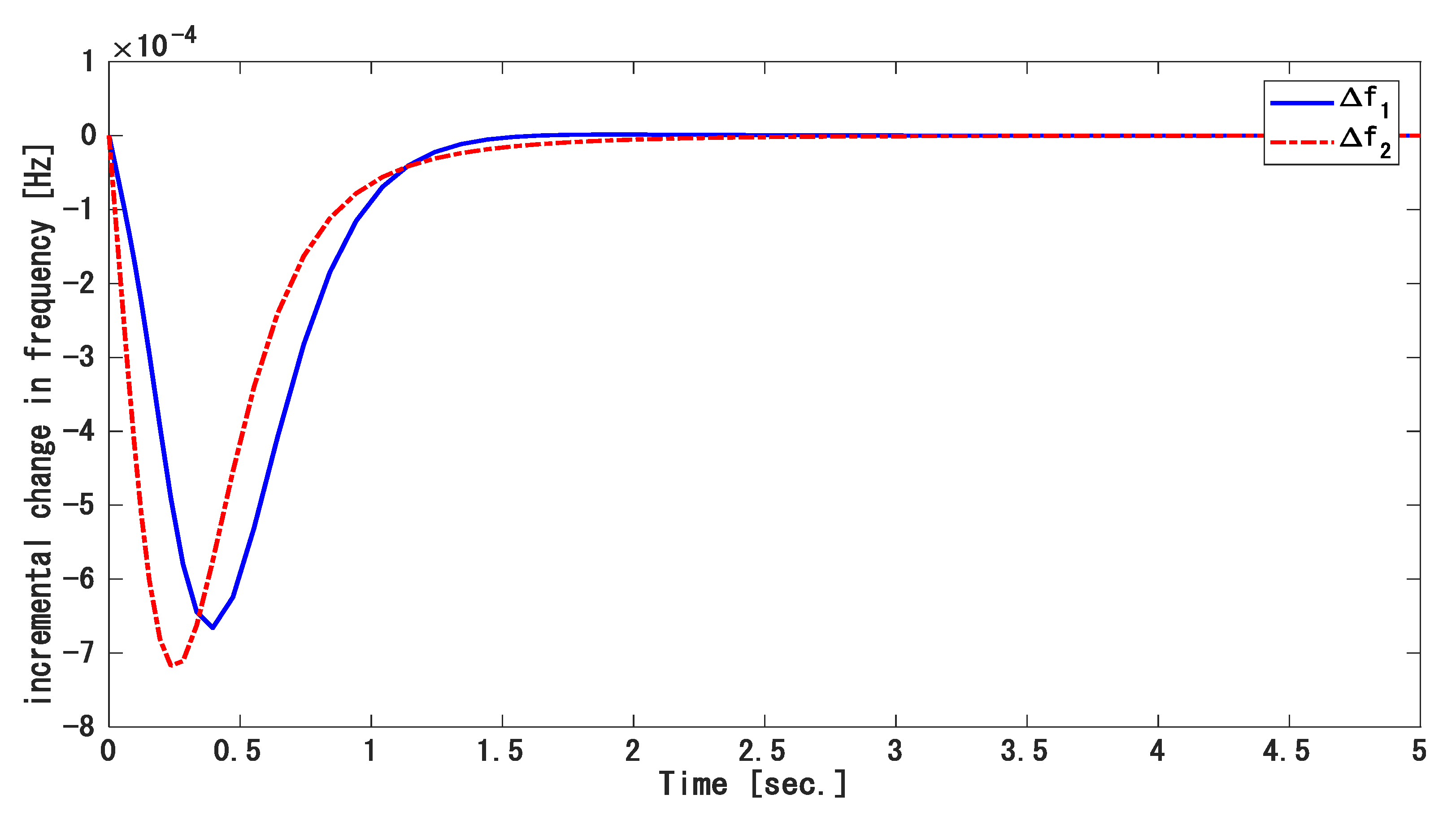
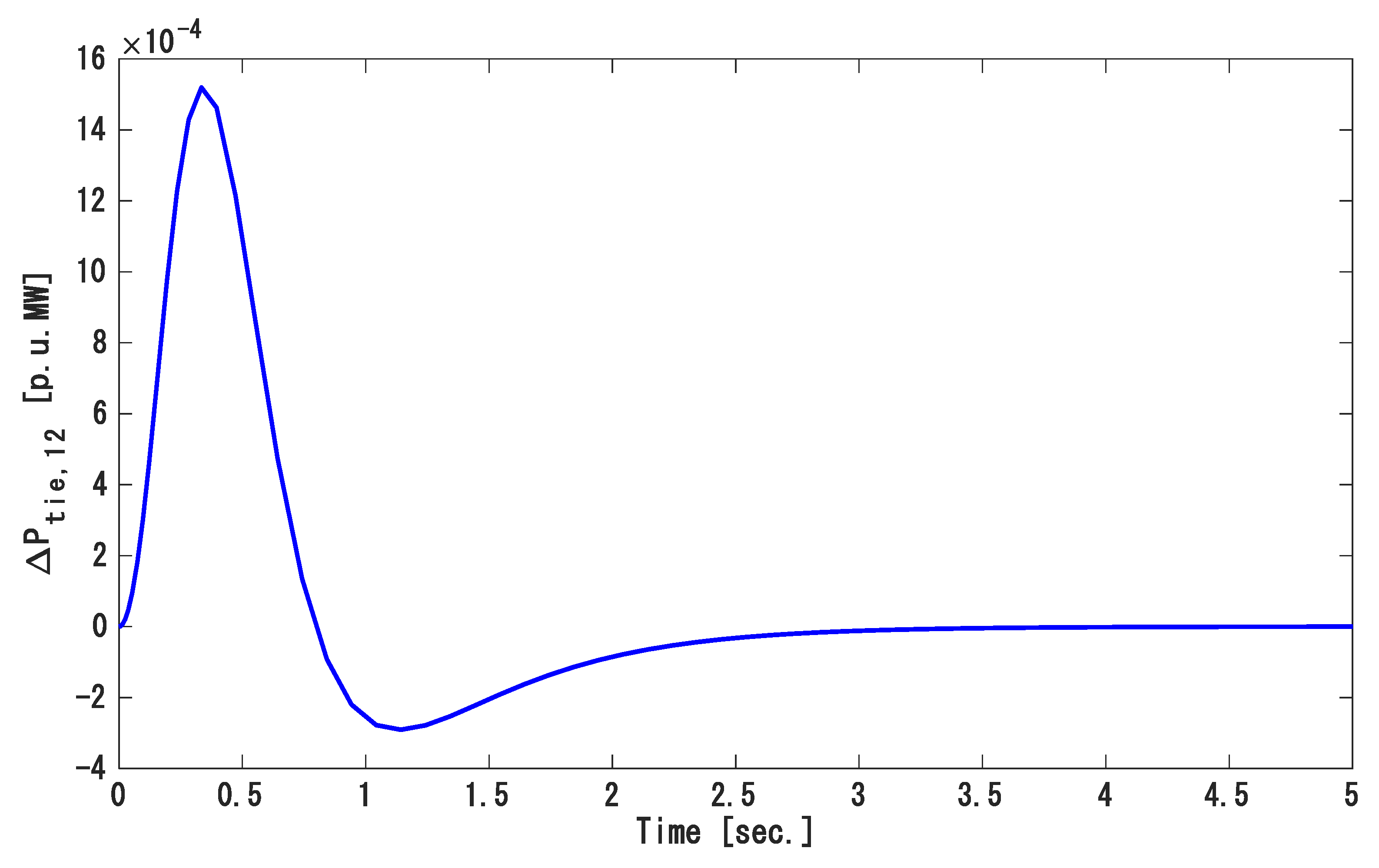
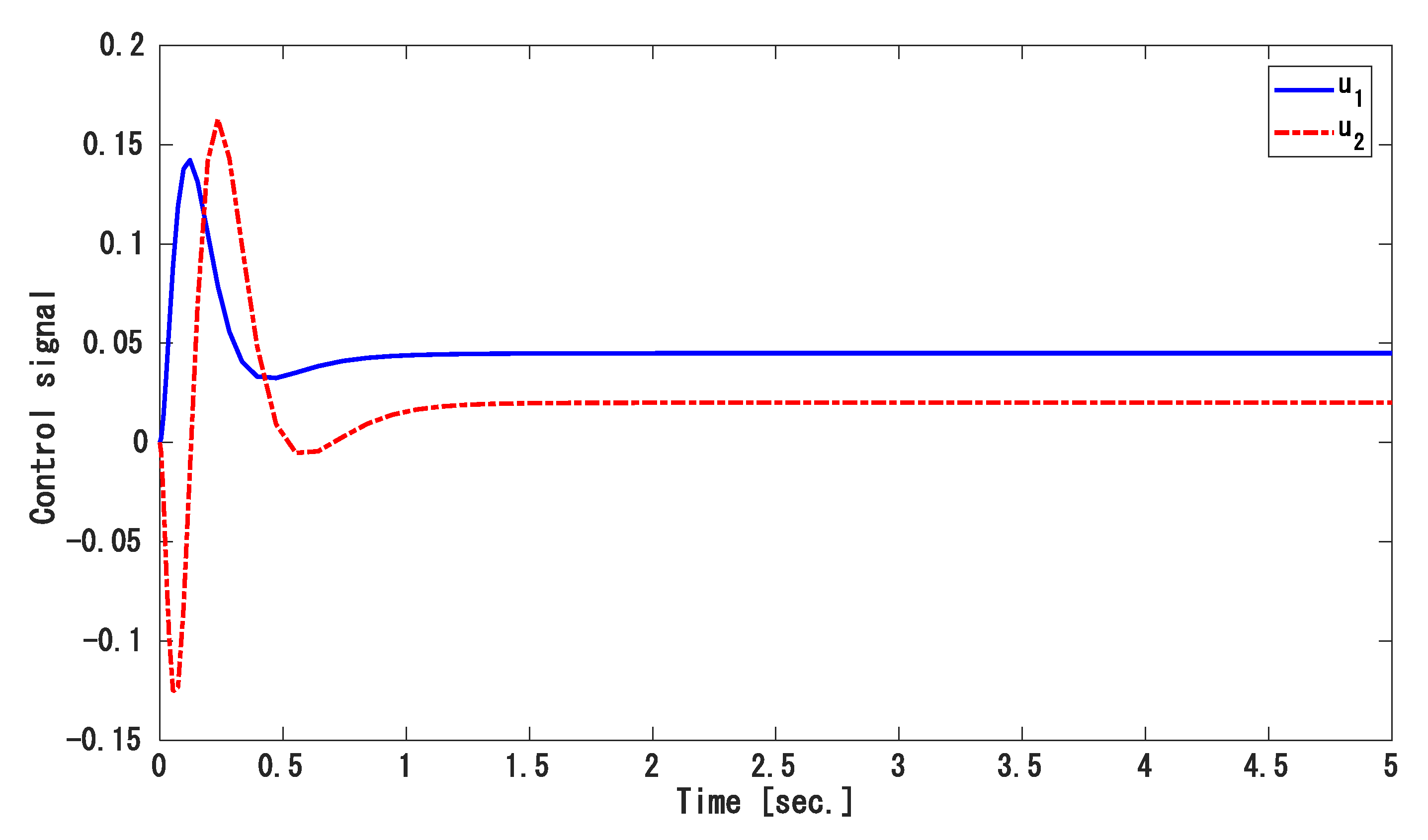
• Case 1: Step load disturbance under a nominal condition.
• Case 2: Step load disturbance under mismatched uncertainty.
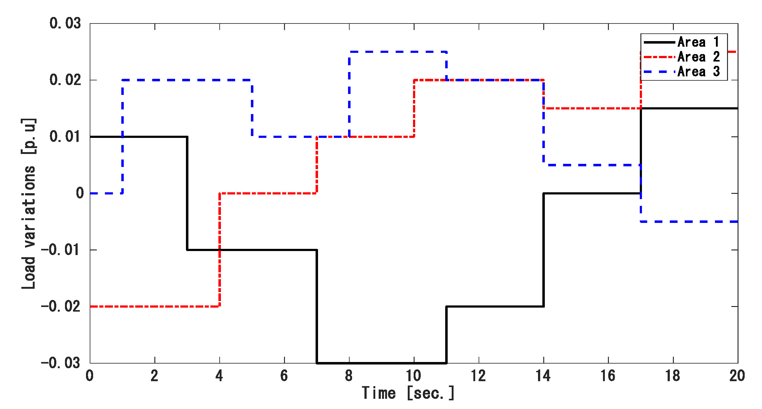
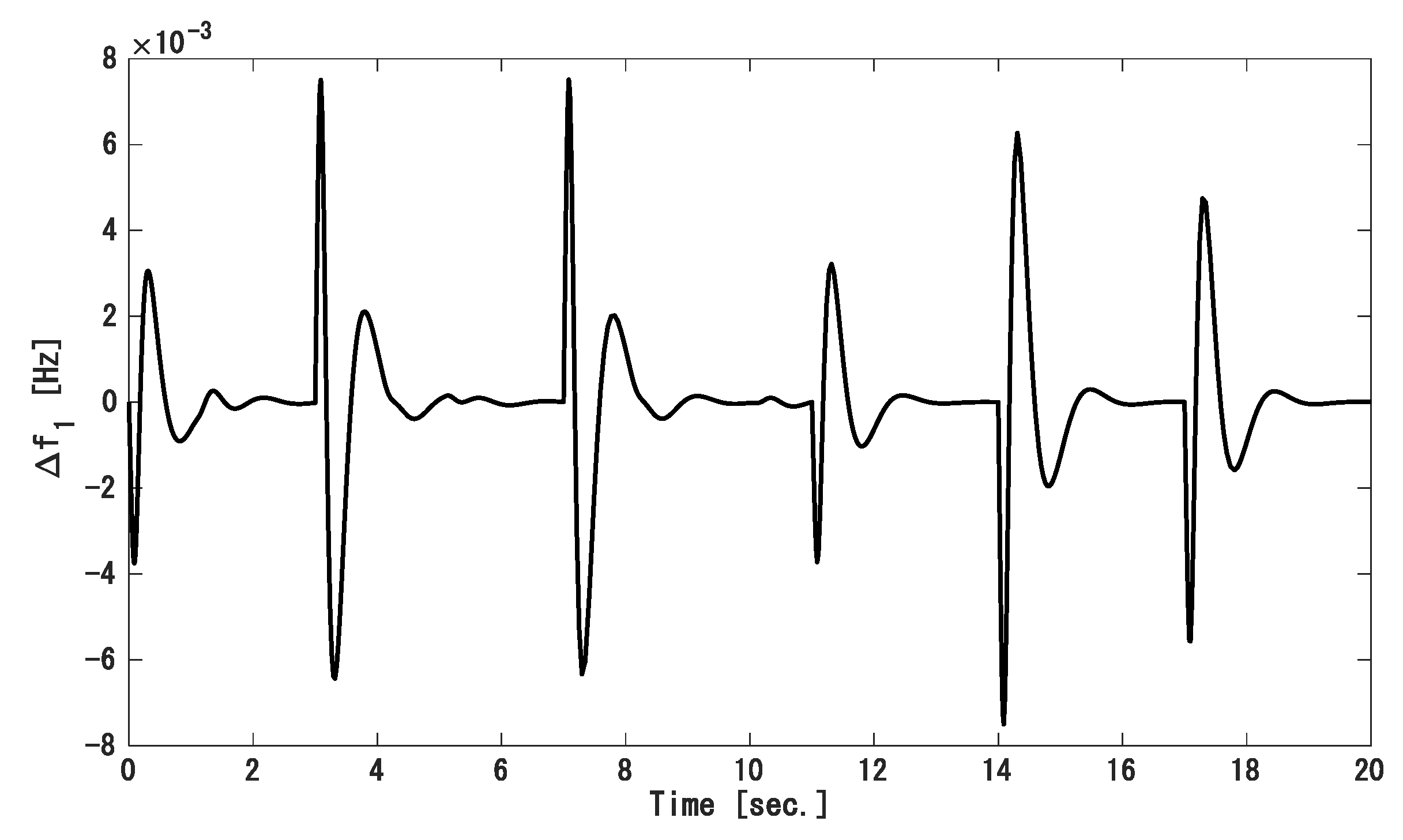
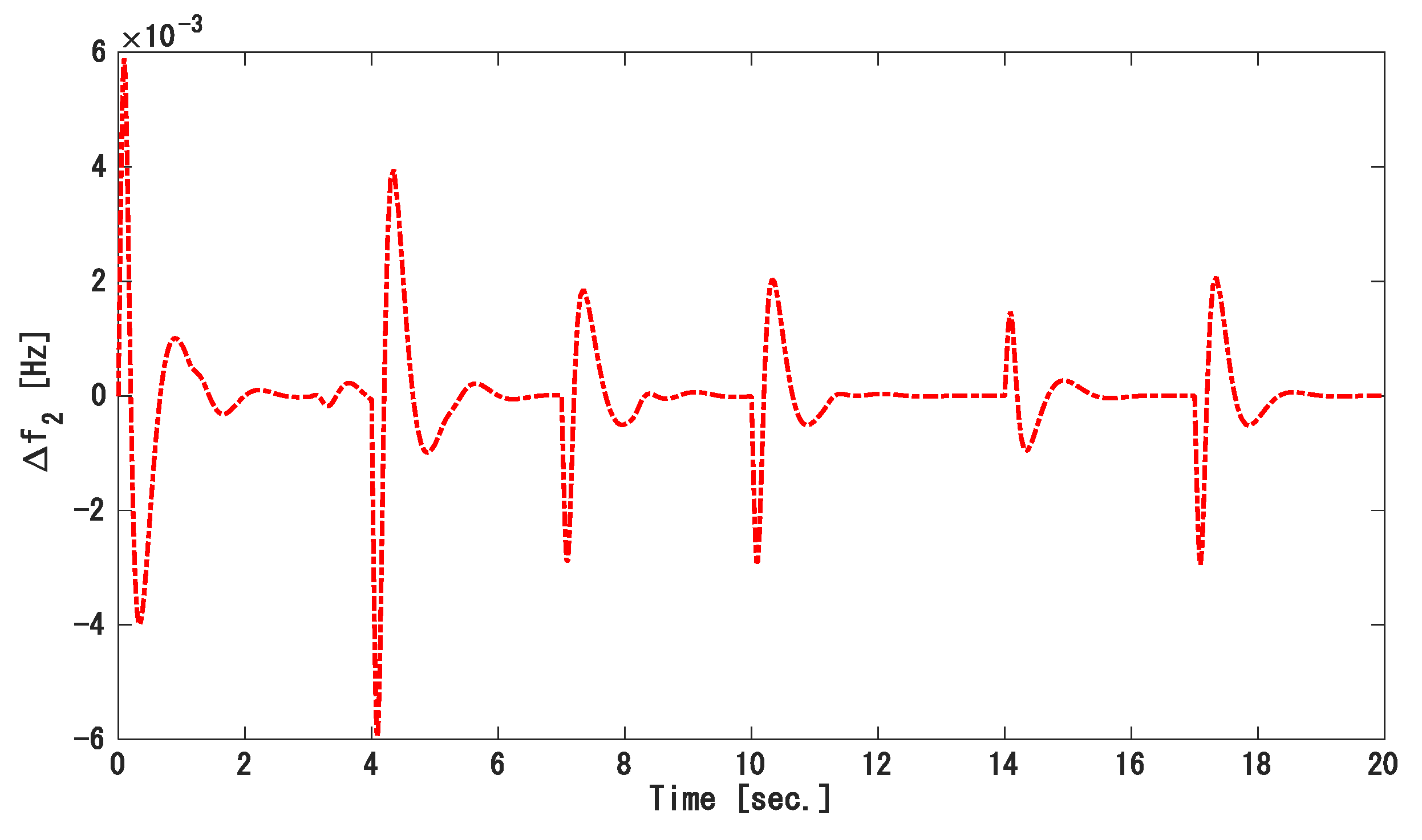
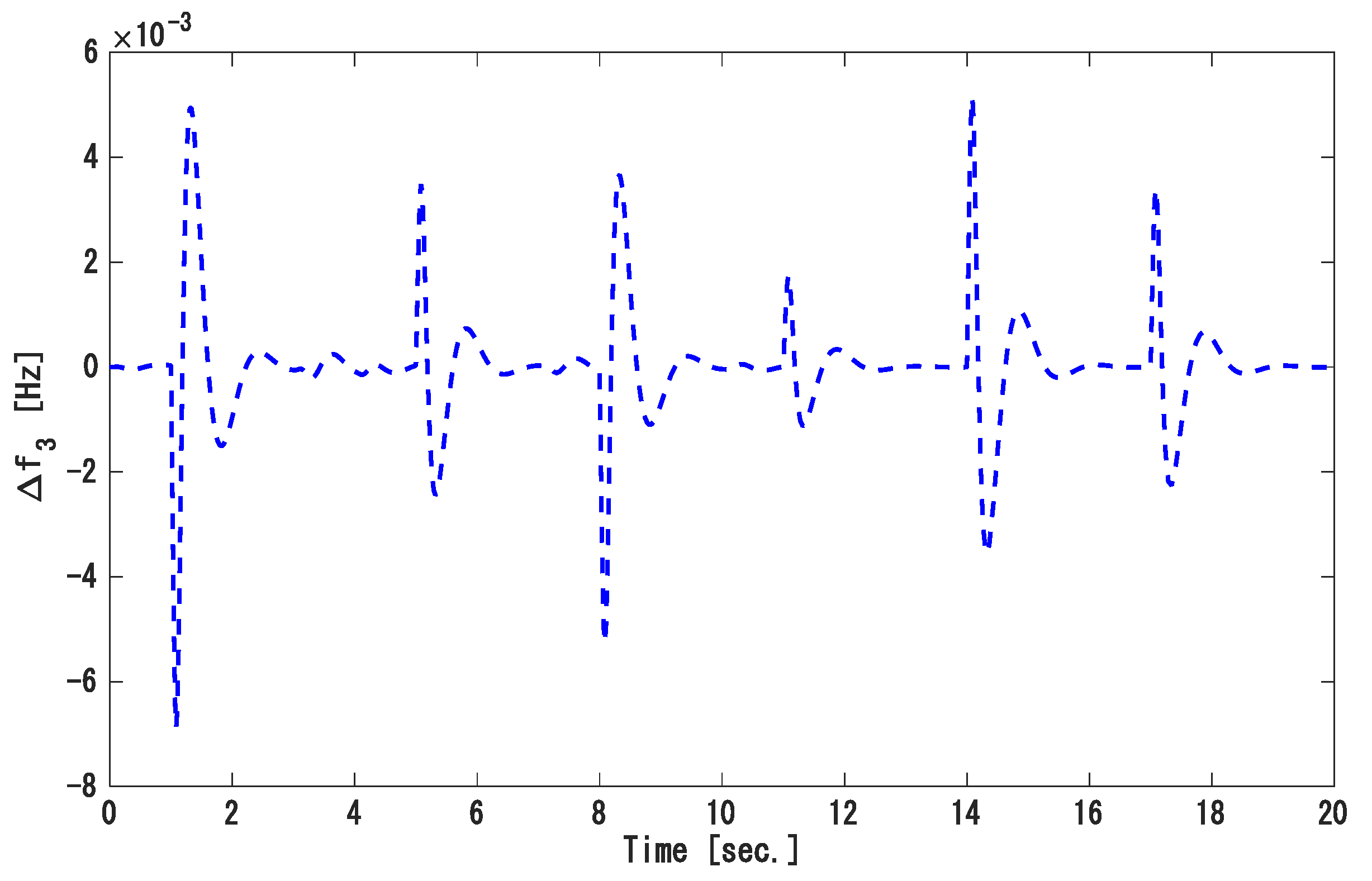
• Case 3: Random load disturbance under mismatched uncertainty.

And their results are compared with ref [31].

• Case 1: Step load disturbance with nominal conditions

First, we simulated the response of the TAPS with SOSMC by introducing a step load change of magnitude $\Delta P_{d1}=0.02(p.uMV)$ in area 1 and $\Delta P_{d2}=0.045(p.uMV)$ in area 2. The frequency divergence in area one (solid line) and area two (dashed line) are illustrated in Figure 2. The tie-line variation is illustrated in Figure 3. The control input signal for area one and two are given in Figure 4.

Frequency and tie-line deviate away from the initial point under the step load. The overshoots seen are damped by the propose controller at a fast response time of 2.5 s. This is achieved by the designed controller gain matrix K in the integral surface. A lack of chattering with control accuracy is also seen in the results, which are due to the SOSMC technique employed. In Figure 4, the small overshoot showed lesser energy used by the designed controller.

Remark 1.

Eventhough we used the information of the system state variables from the observer rather than from the sensor, the frequency deviation and the tie-line power fluctuation are kept in a safer range and the system response is better about under/overshoot and settling time.

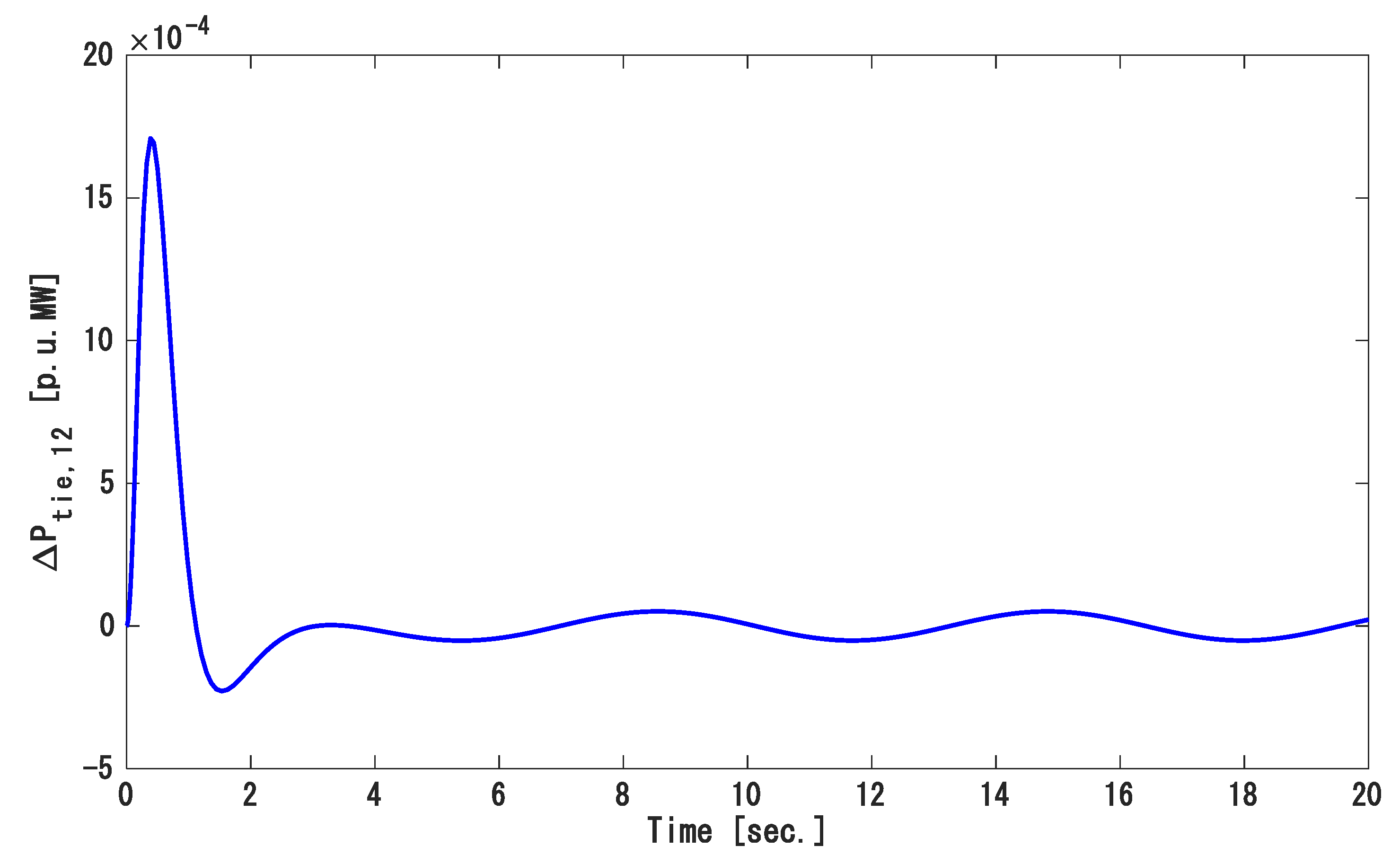
• Case 2. Step load disturbance under the mismatched uncertainty.

The proposed SMC scheme was carried out in the presence of the mismatched condition, and the nonlinear term was linearized to make the model of the system consistent in Figure 1, which consists of deleting some higher order terms, where some error will occur between the real system and the simulation model. The step load disturbances were chosen in the same way as case 1. Furthermore, un-modeled dynamics can degrade the stability of the MAPS. To show the robustness of the new controller, a ± 20% of the nominal value was applied to the system parameters and the un-model dynamic was considered and represented by the cosine function [31]:

$$\Delta A=\left[\begin{array}{ccccccccc}0& 0& 0& 0& 0& 0& 0& 0& 0\\ 0& 0& 0& 0& 0& 0& 0& 0& 0\\ 40\cos (t)& 0& 1.6\cos (t)& 0& 0& 0& 0& 1.6\cos (t)& 0\\ 0& 0& 0& 0& 0& 0& 0& 0& 0\\ 0& 0& 0& 0& 0& 0& 0& 0& 0\\ 0& 0& 0& 0.46\cos (t)& 0& 6\cos (t)& 0& 0& 6\cos (t)\\ 0& 0& 0& 0& 0& 0& 0& 0& 0\\ 0& 0& 0& 0& 0& 0& 0& 0& 0\\ 0& 0& 0& 0& 0& 0& 0& 0& 0\end{array}\right]$$

(38)

The deviation in the frequency of the first and second areas is displayed in Figure 5, and the tie-line power fluctuation is displayed in Figure 6. Figure 7 gives the input of the controller $u_1$ and $u_2$. Once again, at normal operation, the dynamic changes are at zero marks. With the matched condition in the state matrix as shown in [31], both dynamic change values fluctuated, respectively. At 3 s the dynamic spikes were brought to a safe range. The response of the MAPS in terms of the maximum overshoots and settling time are in comparison with [31]. The values of both are written in

Table 2. Setting time and maximum overshoot calculation of SOSMC and observer based SMC [31].

Kind of the Controller	Proposed Method SOSMC		Observer Based SMC [31]
Parameters	$T_s(t)$	Max.O. S (pu)	$T_s(t)$	Max.O. S (pu)
$\Delta f_1$	3	$-5.0\times {10}^{-4}$	7	$-5.0\times {10}^{-4}$
$\Delta f_2$	3	$-6.5\times {10}^{-4}$	7	$-8.0\times {10}^{-4}$

.

Remark 2.

Under the mismatched condition, the proposed controller has good performance in terms of fast response time to bring the dynamic to the zero mark, lesser overshoots seen, and chattering free control without loss of accuracies when compared with [31].

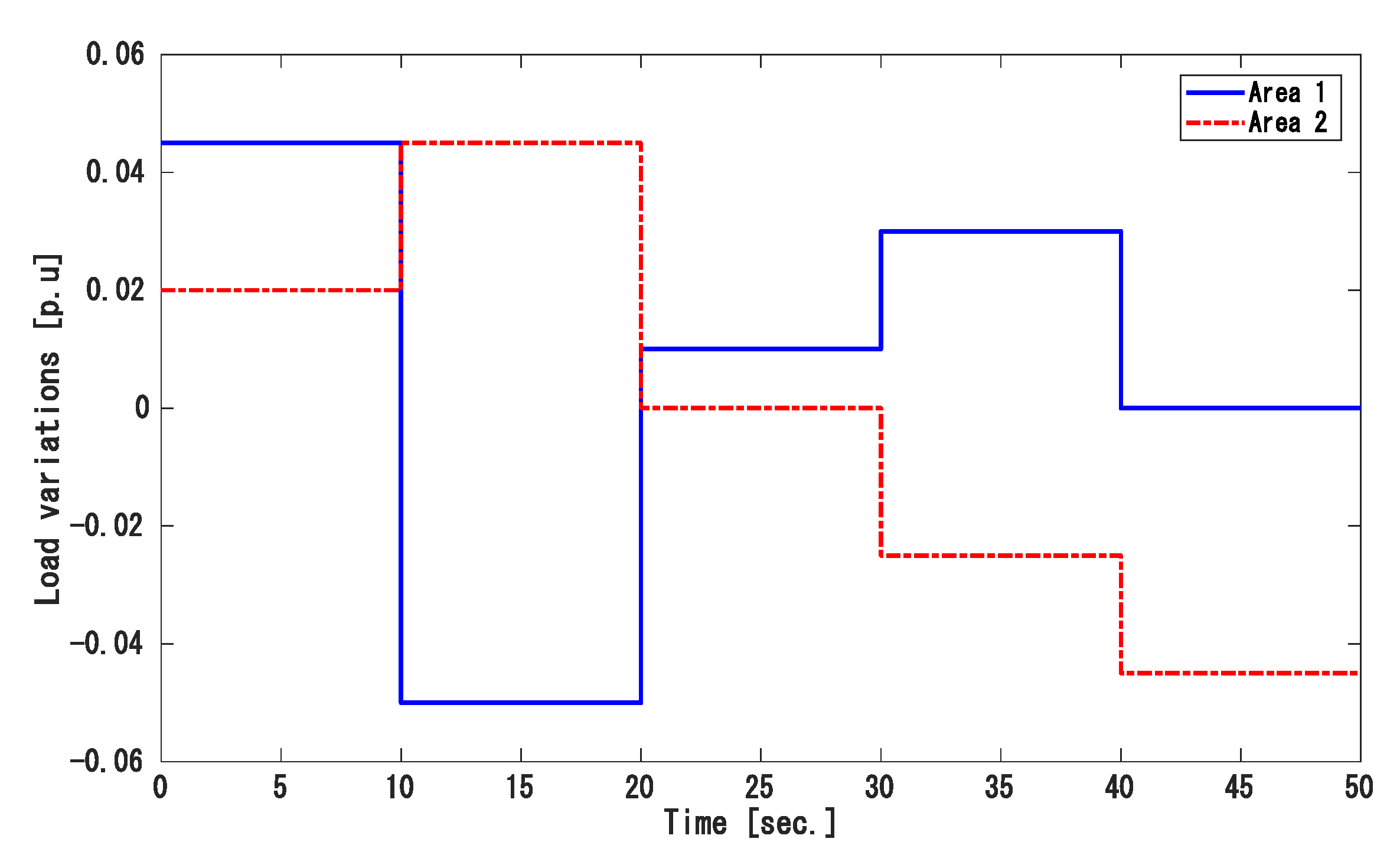
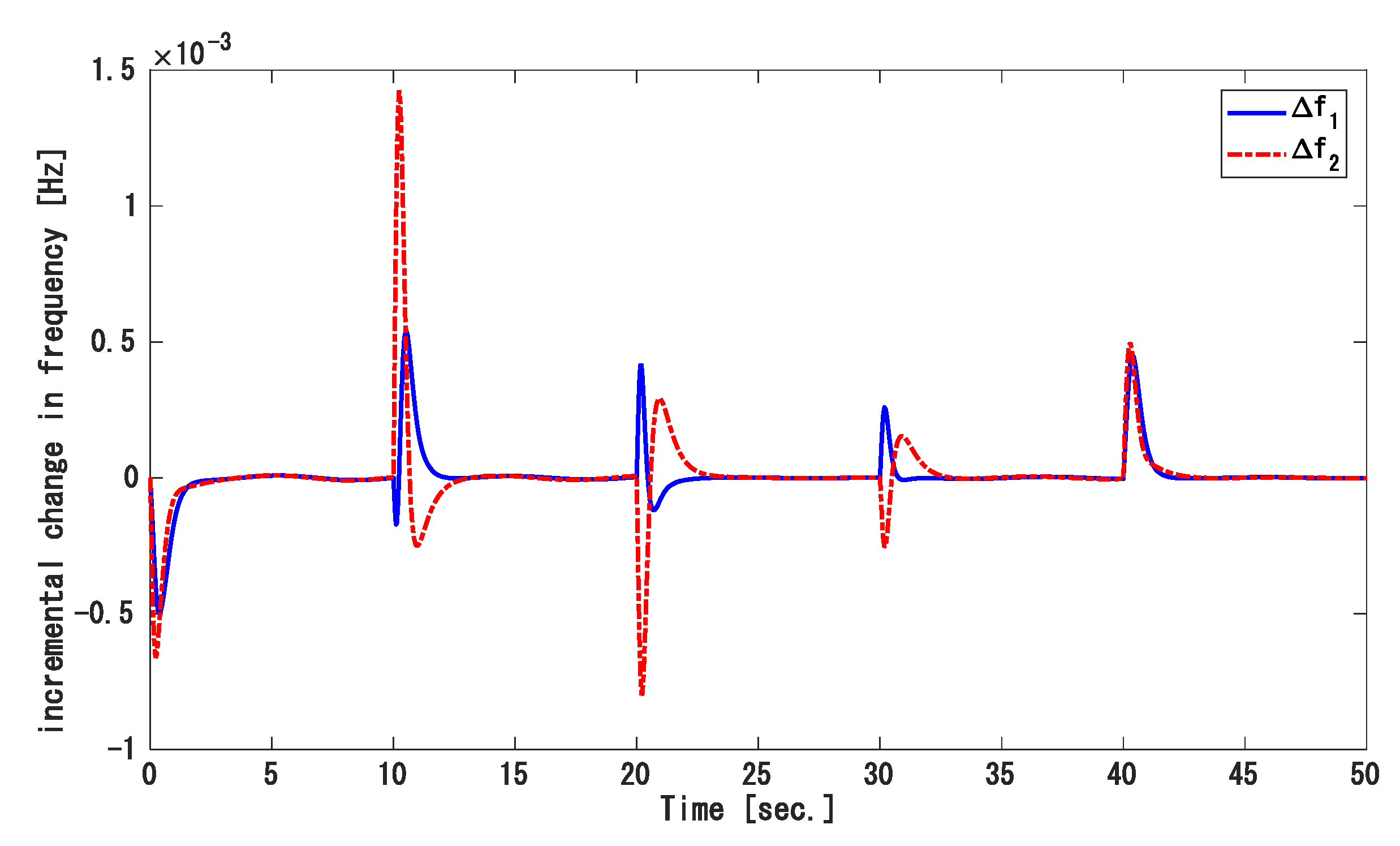
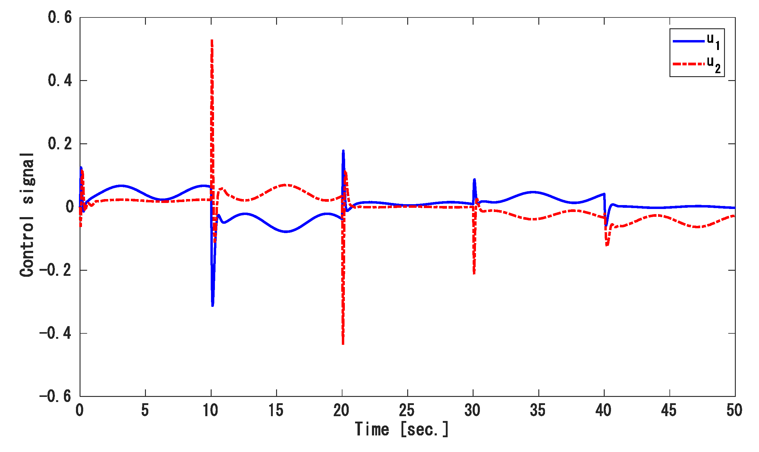
• Case 3. Random load disturbance under mismatched uncertainty

To validate the robustness of the suggested controller, a random load at 10 s intervals was applied to the power plants. We considered a random load variations pattern given in Figure 8, while the mismatched uncertainty was still kept the same as with case 2. Figure 9 shows the frequency divergence. The tie-line power variation is displayed in Figure 10 and the control signals in both areas are displayed in Figure 11.

Thus, the tie-line power deviation and frequency deviation converge to zero by using the sliding surface and the controller based on the state estimator. The response of the power system is better in terms of overshoot even when the system state variables are not measured. Therefore, the new controller can be applied in large power systems.

Remark 3.

Even at random load variation and mismatched uncertainties, the ISS and the controller based on the state observer performed well by keeping the tie-line power and frequency at a safer point at every interval. The response of the power system is better with minimal overshoot which have no effect on damage to the actuator valve.

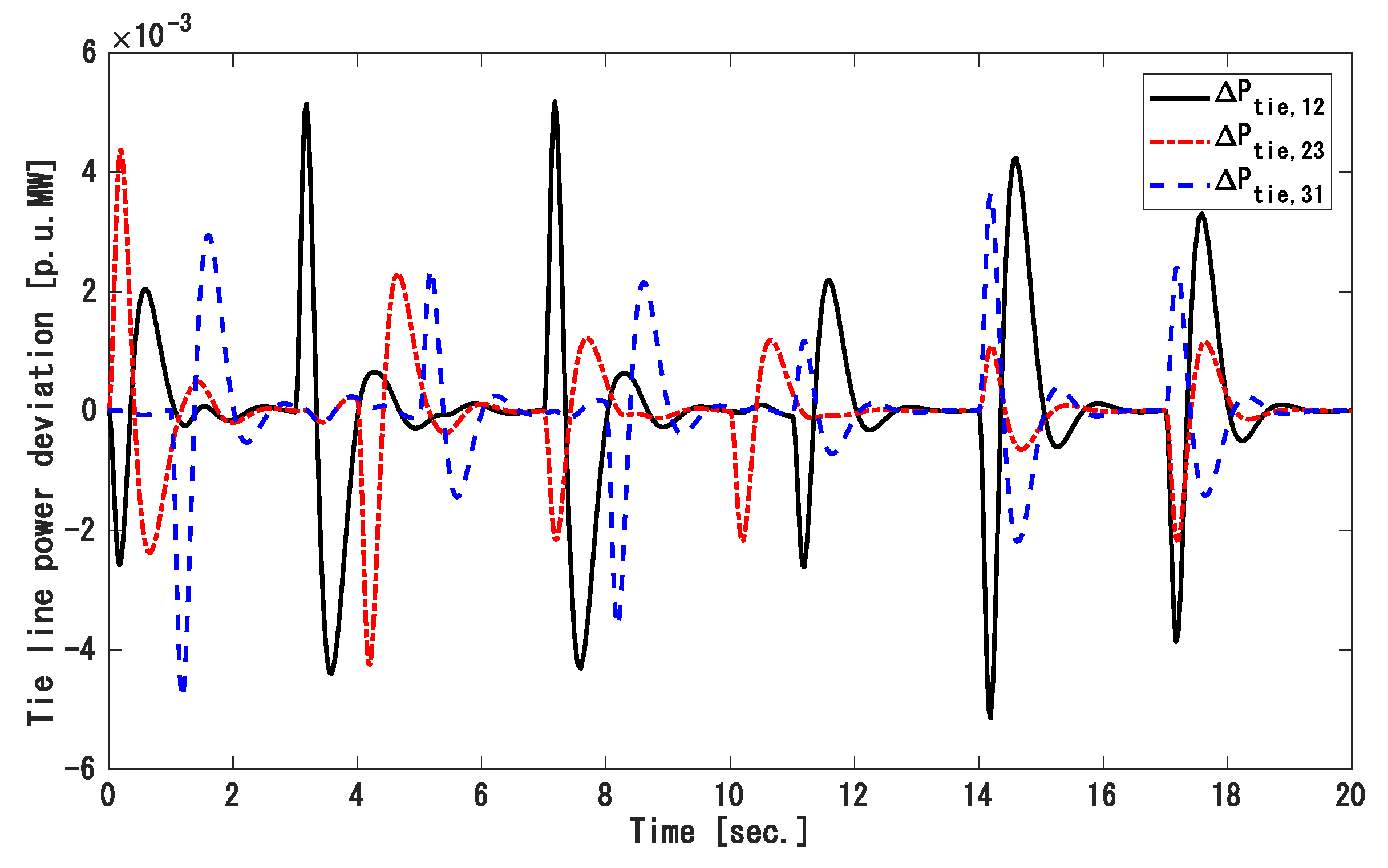
4.2. Simulation 2: England 10 Generation 39 Bus Power System

To extend the proposed controller based on state observer performance, we simulated it in a New England 39 bus system as Figure 12 and system parameters are from [33]. It comprised of three area power systems with 10 generators and 39 bus nodes. All generators were synchronized and connected in parallel.

Because load demands in a real power system keep changing, we applied random load variation in each area as shown in Figure 13. Figure 14, Figure 15 and Figure 16 show the frequency variation of area 1, 2, and 3, respectively, and the tie-line power deviation is displayed in Figure 17. The tie-line power flow and frequency fluctuation rapidly converged to zero even though the system state variables were not measured. Therefore, this approach is better to maintain frequency and tie-line power at a safe range in a large power network where SSV are difficult to measure.

Remark 4.

In this approach, the suggested controller based on observer is tested with a real power network and theresults indicate that the suggested method is powerful for the control of a large power network under load variations depending on time, with fast settling time and small overshoot.

Remark 5.

In general, the proposed method achieved better control performance in terms of keeping tie-line power and frequency at the accepted point for the power system where SSVs are difficult to measure. The proposed scheme is extremely powerful, and not only reduces chattering but also guarantees the robustness of the MAPS.

5. Conclusions

The system state variables are difficult or expensive to measure for load frequency control (LFC) of a multi area power system. In this paper, a new method based on SMC combined with an observer has been proposed to estimate the system state variables for LFC. The estimated state observer is used fully in the sliding surface and continuous second order sliding mode controller, which reduces the chattering problem and improves the system performance. In addition, the new linear matrix inequality technique is derived to prove the stability of the whole system which includes estimated state variables and the real state variables. Experimental simulation results show that the frequency deviation and the tie-line power flow are observed with reduced settling time and magnitude of overshoot in comparison with existing methods in the literature. Furthermore, the second order sliding mode-based observer has been successfully applied for an IEEE 39 bus multi area power system with the load variations, with matched and mismatched uncertainties. Therefore, it can be concluded that the proposed scheme is not only robust in the presence of matched and mismatched uncertainties but also can be successfully applied to a real power system.

References

1. Parmar, K.P.S.; Majhi, S.; Kothari, D.P. Load frequency control of a realistic power system with multi-source power generation. Int. J. Electr. Power Energy Syst. 2012, 42, 426–433. [Google Scholar] [CrossRef]
2. Liu, X.; Nong, H.; Xi, K.; Yao, X. Robust Distributed Model Predictive Load Frequency Control of Interconnected Power System. Math. Probl. Eng. 2013, 15, 10–20. [Google Scholar] [CrossRef]
3. Vittal, V.; Mc Calley, J.D.; Anderson, P.M.; Fouad, A.A. Power System Control and Stability, 3rd ed.; Electric Power Systems: Richardson, TX, USA, 2019; pp. 19–400. [Google Scholar]
4. Tan, W.; Hao, Y.; Li, D. Load frequency control in deregulated environments via active disturbance rejection. Int. J. Electr. Power Energy Syst. 2015, 66, 166–177. [Google Scholar] [CrossRef]
5. Pandey, S.K.; Mohanty, S.R.; Kishor, N. A literature survey on load–frequency control for conventional and distribution generation power systems. Renew. Sustain. Energy Rev. 2013, 25, 318–334. [Google Scholar] [CrossRef]
6. Tan, W.; Zhou, H.; Fu, C. Linear active disturbance rejection control for load frequency control of power systems. Control Theory Appl. 2013, 30, 1607–1615. [Google Scholar]
7. Lu, X.; Yu, X.; Lai, J.; Guerrero, J.M.; Zhou, H. Distributed Secondary Voltage and Frequency Control for Islanded Microgrids with Uncertain Communication Links. IEEE Trans. Ind. Inform. 2017, 13, 448–460. [Google Scholar] [CrossRef] [Green Version]
8. Lim, K.Y.; Wang, Y.; Zhou, R. Robust decentralised load-frequency control of multi-area power systems. IEEE Proc.-Gener. Transm. Distrib. 1996, 143, 377–386. [Google Scholar] [CrossRef]
9. Dong, L.; Zhang, Y.; Gao, Z. A robust decentralized load frequency controller for interconnected power systems. ISA Trans. 2012, 51, 410–419. [Google Scholar] [CrossRef] [Green Version]
10. Alrifai, M.; Hassan, M.; Zribi, M. Decentralized load frequency controller for a multi-area interconnected power system. Int. J. Electr. Power Energy Syst. 2011, 33, 198–209. [Google Scholar] [CrossRef]
11. Pappachen, A.; Fathima, A.P. Critical research areas on load frequency control issues in a deregulated power system: A state-of-the-art-of-review. Renew. Sustain. Energy Rev. 2017, 72, 163–177. [Google Scholar] [CrossRef]
12. Sharma, J.; Hote, Y.V.; Prasad, R. Robust PID Load Frequency Controller Design with Specific Gain and Phase Margin for Multi-area Power Systems. IFAC Pap. 2018, 51, 627–632. [Google Scholar] [CrossRef]
13. Aditya. Design of Load Frequency Controllers Using Genetic Algorithm for Two Area Interconnected Hydro Power System. Electr. Power Compon. Syst. 2010, 31, 81–94. [Google Scholar] [CrossRef]
14. Ramachandran, R.; Madasamy, B.; Veerasamy, V.; Saravanan, L. Load frequency control of a dynamic interconnected power system using generalized Hopfield neural network based self-adaptive PID controller. IET Gener. Transm. Distrib. 2018, 12, 5713–5722. [Google Scholar] [CrossRef]
15. Bevrani, H.; Daneshmand, P.R. Fuzzy logic-based load-frequency control concerning high penetration of wind turbines. IEEE Syst. J. 2012, 6, 173–180. [Google Scholar] [CrossRef]
16. Yousef, H.A.; AL-Kharusi, K.; Albadi, M.H.; Hossetinzadeh, N. Load frequency control of a multi-area power system: An adaptive fuzzy logic approach. IEEE Trans. Power Syst. 2014, 29, 1822–1830. [Google Scholar] [CrossRef]
17. Sinha, S.; Patel, R.; Prasad, R. Application of GA and PSO Tuned Fuzzy Controller for AGC of Three Area Thermal-Thermal-Hydro Power System. Int. J. Comput. Theory Eng. 2010, 2, 238–244. [Google Scholar] [CrossRef]
18. Daneshfar, F.; Bevrani, H. Multiobjective design of load frequency control using genetic algorithms. Int. J. Electr. Power Energy Syst. 2012, 42, 257–263. [Google Scholar] [CrossRef]
19. Rahman, M.M.; Chowdhury, A.H.; Hossain, M.A. Improved load frequency control using a fast acting active disturbance rejection controller. Energies 2017, 10, 1718. [Google Scholar] [CrossRef] [Green Version]
20. Vijaya Chandrakala, K.R.M.; Balamurugan, S.; Sankaranarayanan, K. Variable structure fuzzy gain scheduling based load frequency controller for multi area hydro thermal system. Int. J. Electr. Power Energy Syst. 2013, 53, 375–381. [Google Scholar] [CrossRef]
21. Yang, B.; Yu, T.; Shu, H.; Yao, W.; Jiang, L. Sliding-mode perturbation observer-based sliding-mode control design for stability enhancement of multi-machine power systems. Trans. Inst. Meas. Control 2018, 41, 1418–1434. [Google Scholar] [CrossRef]
22. Pradhan, S.K.; Das, D.K. H∞ Load Frequency Control Design Based on Delay Discretization Approach for Interconnected Power Systems with Time Delay. J. Mod. Power Syst. Clean Energy 2020. [CrossRef]
23. Sun, Y.; Wang, Y.; Wei, Z.; Sun, G.; Wu, X. Robust H∞ Load Frequency Control of Multi-Area Power System with Time Delay: A Sliding Mode Control Approach. IEEE/Caa J. Autom. Sin. 2018, 5, 610–617. [Google Scholar] [CrossRef]
24. Mi, Y.; Fu, Y.; Wang, C.; Wang, P. Decentralized Sliding Mode Load Frequency Control for Multi-Area Power Systems. IEEE Trans. Power Syst. 2013, 28, 4301–4309. [Google Scholar] [CrossRef]
25. Huynh, V.V.; Minh, B.L.N.; Amaefule, E.N.; Tran, A.-T.; Tran, P.T. Highly Robust Observer Sliding Mode Based Frequency Control for Multi Area Power Systems with Renewable Power Plants. Electronics 2021, 10, 274. [Google Scholar] [CrossRef]
26. Huynh, V.V.; Tran, P.T.; Minh, B.L.N.; Tran, A.-T.; Tuan, D.H.; Nguyen, T.M.; Vu, P.T. New Second-Order Sliding Mode Control Design for Load Frequency Control of a Power System. Energies 2020, 13, 6509. [Google Scholar] [CrossRef]
27. Wei, Z.; Dong, G.; Zhang, X.; Pou, J.; Quan, Z.; He, H. Noise-Immune Model Identification and State-of-Charge Estimation for Lithium-Ion Battery Using Bilinear Parameterization. IEEE Trans. Ind. Electron. 2020, 68, 312–323. [Google Scholar] [CrossRef]
28. Wei, Z.; He, H.; Pou, J.; Tsui, K.L.; Quan, Z.; Li, Y. Signal-Disturbance Interfacing Elimination for Unbiased Model Parameter Identification of Lithium-Ion Battery. IEEE Trans. Ind. Inform. 2020. [CrossRef]
29. Chen, C.; Zhang, K.; Yuan, K.; Wang, W. Extended partial states observer based load frequency control scheme design for multi-area power system considering wind energy integration. IFAC Pap. 2017, 50, 4388–4393. [Google Scholar] [CrossRef]
30. Mi, Y.; Fu, Y.; Li, D.; Wang, C.; Loh, P.C.; Wang, P. The sliding mode load frequency control for hybrid power system based on disturbance observer. Int. J. Electr. Power Energy Syst. 2016, 74, 446–452. [Google Scholar] [CrossRef]
31. Prasad, S.; Purwar, S.; Kishor, N. Load frequency regulation using observer based non-linear sliding mode control. Int. J. Electr. Power Energy Syst. 2019, 104, 178–193. [Google Scholar] [CrossRef]
32. Dev, A.; Sarkar, M.K. Robust higher order observer based non-linear super twisting load frequency control for multi area power systems via sliding mode. Int. J. Control Autom. Syst. 2019, 17, 1814–1825. [Google Scholar] [CrossRef]
33. Liao, K.; Xu, Y. A robust load frequency control scheme for power systems based on second-order sliding mode and extended disturbance observer. IEEE Trans. Ind. Inform. 2017, 14, 3076–3086. [Google Scholar] [CrossRef]
34. Tsai, Y.W.; Huynh, V.V. A multitask sliding mode control for mismatched uncertain large-scale systems. Int. J. Control 2015, 88, 1911–1923. [Google Scholar] [CrossRef]
Figure 1. Schematics of TAPS interconnection.
Energies 14 00863 g001
Figure 2. The frequency variation.
Energies 14 00863 g002
Figure 3. The tie-line power deviations.
Energies 14 00863 g003
Figure 4. Control signal.
Energies 14 00863 g004
Figure 5. The frequency deviations.
Energies 14 00863 g005
Figure 6. Tie line power deviation.
Energies 14 00863 g006
Figure 7. Control signal.
Energies 14 00863 g007
Figure 8. Random load variation.
Energies 14 00863 g008
Figure 9. The frequency variation.
Energies 14 00863 g009
Figure 10. Tie-line power variation.
Energies 14 00863 g010
Figure 11. Control signal.
Energies 14 00863 g011
Figure 12. New England test system.
Energies 14 00863 g012
Figure 13. Random load variation.
Energies 14 00863 g013
Figure 14. The frequency variation of 1st area.
Energies 14 00863 g014
Figure 15. The frequency variation of 2nd area.
Energies 14 00863 g015
Figure 16. The frequency deviation of 3rd area.
Energies 14 00863 g016
Figure 17. Tie-line variation of 3 areas.
Energies 14 00863 g017