Abstract
Peak-shaving is a very efficient and practical strategy for a day-ahead hydropower scheduling in power systems, usually aiming to appropriately schedule hourly (or in less time interval) power generations of individual plants so as to smooth the load curve while enforcing the energy production target of each plant. Nowadays, the power marketization and booming development of renewable energy resources are complicating the constraints and diversifying the objectives, bringing challenges for the peak-shaving method to be more flexible and efficient. Without a pre-set or fixed peak-shaving order of plants, this paper formulates a new peak-shaving model based on the mixed integer linear programming (MILP) to solve the scheduling problem in an optimization way. Compared with the traditional peak-shaving methods that need to determine the order of plants to peak-shave the load curve one by one, the present model has better flexibility as it can handle the plant-based operating zones and prioritize the constraints and objectives more easily. With application to six cascaded hydropower reservoirs on the Lancang River in China, the model is tested efficient and practical in engineering perspective.
1. Introduction
In a power system, power generation must match the load all the time, which means the power resources should adjust their own output synchronously to satisfy the real-time load demands. The peak-shaving, a short-term scheduling strategy, aims at scheduling the hourly generations of plants to smooth the load curve of a power system with various constraints enforced, including, for example, the power balance and power generation targets. Nowadays, power systems, with thermal, hydropower and other energy resources involved, are becoming more and more complex. In the past few decades, energy demand has been experiencing a booming expansion period with the development of both the society and the economy [1]. However, the concerns about global environmental issues and the risk of energy crisis have limited the utilization of fossil energy resources, which are dominating power sources at present [2]. The development of clean and renewable energies will be an effective measure to resolve the dilemma [3]. Actually, the wind and solar energies will very likely become the mainstream electricity sources and are increasingly cost-competitive compared to fossil fuel power plants [4]. It should be noticed that, with significant volatility, randomness and intermittence, the penetration of large-scale wind and photovoltaic powers will sharply increase the peak-shaving pressure for power systems [5]. It is more complicated in balancing the electric power and energy, which is essential in peak-shaving scheduling. Due to the advantages of flexibility in startup and shutdown, quick response in changing condition, and high reliability, hydropower has an outstanding strength in peak-shaving. On the contrary, with poor regulation abilities, the frequent power fluctuations of thermal plants will lead to unnecessary operational expense for power systems [6,7]. In addition, the variable production of non-dispatchable wind and solar powers requires flexible generation to stabilize the output and the hydropower can supply energy with not only dispatchable flexibility but also fast regulation [8]. As short-term effects become increasingly important due to large-scale integration of renewable energy sources, the proper modelling of a hybrid power system, especially with flexible hydropower, is all-important [9].
The peak-shaving method originates from the heuristic idea that it is more economical to allocate hydro energy to the upper-most part of the system load which corresponds to the peak loads [10]. Meanwhile, thermal plants generate baseload power output, being able to run at high efficiency. The wind and solar powers are considered to run as forecasted. The peak-shaving optimization is executed with the power generation target, available capacity of power sources and unit maintenance plans all known, but the hydraulic constraints for hydropower generation omitted provisionally. The balance of electric power and energy is the primary goal of peak-shaving optimization. The principle of the method is to utilize the system daily load curve and power cumulative curve simultaneously, finding appropriate working position for every power plant in an iterative process. The generation schedules of plants are arranged one by one according to their capacity factor [11], which is defined as the ratio of target energy of the plant to the multiplication of plant capacity by the study period. The plant with lowest capacity factor has relatively high capacity. It is advantageous to apply this plant first, such that the plant capacity can be effectively utilized. The peak-shaving method has been tested efficient and practical, with related applications having been widely reported in previous literature. R.N. Wu et al. [11] investigated the characteristics of the peak-shaving method and the method has been compared with the rigorous coordination-equation method, showing results that the peak-shaving method tends to smooth the equivalent thermal load more effectively and is superior in computation speed. Simopoulos et al. [10] proposed an enhanced peak-shaving method for short-term hydrothermal scheduling problem. The short-term mixed energy system scheduling problem is decomposed into hydro sub-problem and other type sub-problems where hydro sub-problem can be solved by traditional peak-shaving method for the first step, then with the coupling hydraulic constraints enforced later. The focus is the existing peak-shaving methods need to determine a power plant’s ranking order in advance. With the ranking order fixed, the load distribution results may not be practical or need further refinement, and the pre-set working position of a power plant makes it difficult to take advantage of the complementarity among plants. Meanwhile, the increasing load demand and the renewable power resources enlarge the peak-shaving pressure on hydro systems and require for the peak-shaving model to be more flexible.
To achieve multiple objectives, the peak-shaving procedure can also be integrated into a regular optimization model in the form of a series of constraints, such as restricting the valley-peak load ratio [6] or minimizing the fluctuation of residual load. This paper made a great effort to investigate the feasibility of mathematical programming methods to replace the original method. Inspired by the process of traditional peak-shaving method, objective function and constraints have been tactfully designed so that the peak-shaving scheduling can be expressed as a mathematical programming problem. By analyzing the characteristics of different power plants and setting parameters accordingly, all the power plants can participate in peak-shaving at the same time, avoiding the influence of the ranking order on the load distribution results. As for unit commitment, for simplification, this work assumes that every unit’s feasible operating zone is fixed and the units belong to the same plant are grouped as an equivalent one. As done in many existing literatures [12,13], binary variables are involved to express the interval constraints in this work. The solution efficiency of the model is guaranteed by employing professional mathematical programming solver that can deal with MILP problem easily.
The remainder of this paper is organized as follows: Section 2 presents the mathematical formulation of the proposed problems. Then, solution procedures are described in Section 3. With application to the Lancang hydropower cascade consisting of six major reservoirs; results and discussions of case studies are presented in Section 4 and Section 5 concludes this work.
2. Model
The peak-shaving scheduling is a complex mixed-integer non-linear optimization problem. With reasonable simplification, this work introduces binary variables to solve the problem with an MILP formulation. The model takes hydropower plants as example but is also suitable to include other plants. In this part, the model is expressed in mathematical terms and then reformulated as one that can be solved with an MILP solver.
2.1. Model Formulation
2.1.1. Objective Function
The Peak-shaving is supposed to arrange the power output of every plan while meeting the generation limits of its hydropower units. At the same time, the power output process is requested to be as smooth as possible to meet the safety standards. From the peak-shaving standpoint, the power generation process should remain unchanged at the working capacity whenever it is possible, or lower than this working capacity if it is impossible. The objective involves two sub-objectives to:
- Minimize the power output variation:where N and T are the number of plants and periods, respectively; and are the output increase and decrease in MW of plant i from period t-1 to period t, respectively. In other words, this objective aims to minimize the output fluctuation between two adjacent time steps;
- Minimize the distance to the working capacity:where represents the distance of the scheduled output to the expected working capacity in MW of plant i in time period t.
2.1.2. Operational Constraints
The power output process should meet the constraints on generating units, and the generation of all plants should match the system loads simultaneously. In addition, the trend of the power output of each plant should be consistent with the system load so that the major peak-shaving plants can work with ease to balance the deficit to the load demand. The constraints include:
- The power generation target, which requires for the total produced energy to meet the electric quantity determined by operators or trade clearance, expressed as:where denotes the length of one time step in hours. is the power output in MW of plant i in time period t. is the target or transactional energy in MWh of power plant i;
- The power balance, requiring for the total power output of all plants to match the system load in any time interval t, which is expressed as:where is the load demand in MW in period t;
- The distance to the working capacity, which, corresponding to Equation (2), is expressed as:where is the expected working capacity in MW of power plant i, and is the theoretical upper bound on power output in MW of plant i;
- The feasible operating zones for a plant to generate in the lower and upper bounds in each time step, expressed as:where and denote the upper and lower bounds of power output in MW in operating zone j of plant i respectively, and is the number of operating zones of power plant i;
- The trend of power output, making plants share the peak-shaving pressure, expressed as:where period τ represents every possible time periods when system load in t is bigger than that in τ. By sorting the values of system load, the sets of τ with respect to any time period t can be found out. This constraint ensures the power output of each plant not to enlarge the peak-valley differences.
2.2. Model Reformulation
A nonlinear programming cannot guarantee the global optimum be found in theory, but linear programming does. Once the objective function and constraints are expressed linearly, it is capable of obtaining the optimal solution [5]. In this section, the nonlinear constraints are restructured to establish a MILP model which can then be programed and solved more easily.
2.2.1. Operation Constraints Reformulation
It is very likely that when a mathematically feasible solution cannot be achieved, engineers of hydropower reservoirs generally prefer violating some soft constraints in order of priority, such that a satisfactory solution to the real-world problem can always be guaranteed [14]. Considering that in the real-world dispatching operation, slight violations of the power generation over its bounds or other constraints are permitted. This work reconstructs some constraints to be relaxed. Thus, constraints can be classified into two types: the prioritized constraints and hard ones. The prioritized constraints are relaxed with extra variables while the hard constraints must be met in any case [14]. The nonlinear constraints are approximated into linear constraints by introducing integer variables.
The constraints after reconstruction include:
- The energy target during the scheduling horizon:where and are positive and negative deviations from the target energy production in MWh of plant i, respectively, of which only one can and will be greater than zero;
- Hourly load balance:
- The power output ramping:
- The working capacity. As shown in Equation (5), the constraint should be satisfied for all time periods which is actually not necessary or possible in some cases and can be simplified. When there is at least one unit online, indicating the power output is greater than zero, the output should meet the working capacity constraint. By introducing a binary variable, the constraint can be reconstructed as below:where is a binary variable representing the operating state of hydro plant i in period t, which is equal to 1 when the plant is online and 0 otherwise. M is a sufficiently large number relative to system load and can be assigned to twice the peak load;
- The operating zones:where represents whether power plant i runs in operating zone j in period t, and Equation (16) means one operating zone at most is workable at any given time for any plant committed;
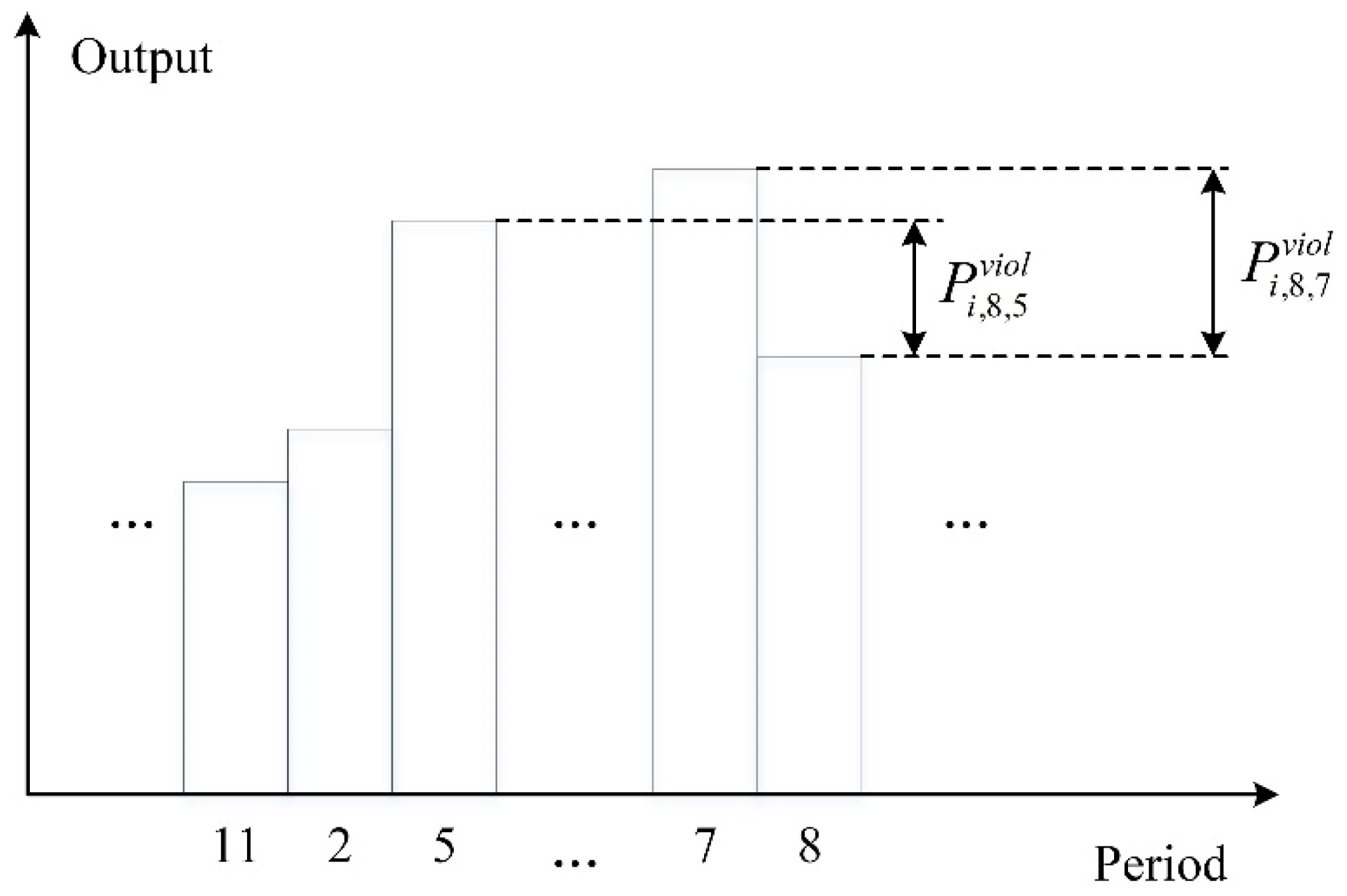
- The power output constraints across different periods:where in MW indicates that the output of plant i in t plus can be greater than the output in τ. is the accumulative value of over different τ. In other words, represents a kind of violation over the constraint that the trend of power output of each plant should be consistent with the system load and hereafter will be only referred to as Trend Violation Item (TVI). Figure 1 demonstrates the meaning of TVI while the time periods on horizontal axis has been sorted in ascending order for system load values.
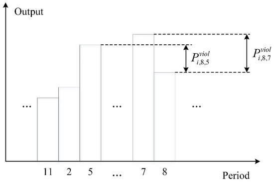 Figure 1. An example of trend violation item (TVI).
 - Non-negative constraint, enforced on all the variables to be nonnegative.
2.2.2. Objective Function Reformulation
With the operational constraints reformulated, the original objective expands to be minimizing: the energy target deviations, the output ramping of power plants, the working capacity violation, and the TVI. The objectives are prioritized and optimized sequentially in descending order of priority, which means that improving one objective will not sacrifice any objective in higher priority. Through optimizing the sum of objectives with various weights, the task can be achieved, and the final objective function is expressed as:
where , , , and are weights assigned to the objectives, different in magnitude, decided according to the importance of each sub-objectives for the dispatching authority; coefficient is an additional coefficient for power plant i and is designed to roughly reflect the role of the plant in balancing the system load. The smaller the coefficient is, the closer is the position to the top in the system load curve. Generally speaking, the value of this coefficient is decided by the plant’s peaking-shaving ability and other characteristics.
2.3. Applicability of the Model
The method proposed is suitable for balancing hourly (or in less time interval) power demands within a day in a power system consisting of hydro and other power plants that have the capability of regulating their hourly generation within the day. For a large-scale hydropower system, the water balance is assumed to be satisfied by controlling the total energy production of each plant in a daily scale. In other words, the water balance or hydraulic constraints of cascaded hydropower plants have been taken into consideration in medium-term generation scheduling. Accordingly, this work enforces the constraint on daily total energy production and hourly power balance while ignoring the hourly water balance within the day. This simplification is feasible for load balance and scheduling within a day of large-scale hydropower systems in the real world.
3. Model Solving Method
As there has been many mature mathematical solvers developed, for example, ILOG CPLEX and Gurobi, the global optimal solution of the MILP model can be obtained in reasonable time. The MILP has been widely used in power dispatching field. G. W. Chang et al. [15] proposed a practical approach for unit commitment and solved the problem via CPLEX. B. Tong et al. [16] built a short-term hydro generation scheduling model based on the MILP and analyzed the linearization effects on solution, the results show that the solution obtained based on the approximated MILP formulation remains feasible for the original nonlinear formulation. This study develops a novel and effective peak-shaving model also based on MILP to determine the generation scheduling of hydropower plants with variable peak-shaving order while satisfying the power and energy balance constraints.
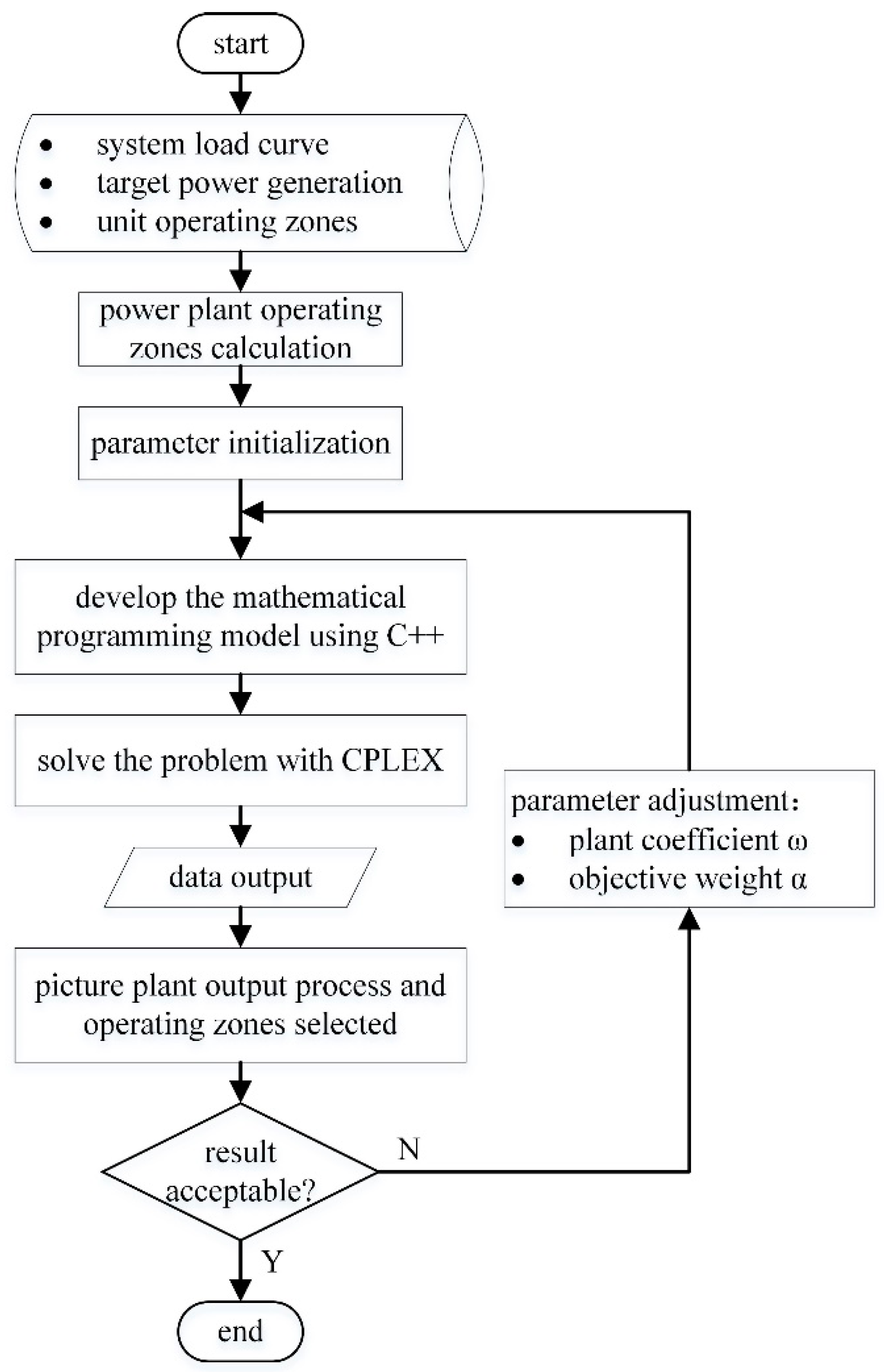
Figure 2 shows the model establishment and solving process in this work. The solution procedure has two main steps. First, this model is coded in C++: the purpose of programming is not only to express the model accurately but also to eliminate some invalid constraints to reduce the computational burden [17]. Second, the model is solved using the CPLEX Optimizer through C++ application programming interface (API). The CPLEX optimizer solves MILP model using a very general and robust algorithm based on branch and cut. While the MILP models have the potential to be much more difficult than their continuous LP, QCP, and QP counterparts, it is also the case that large MILP models are routinely solved in many industrial applications. By this way, it provides a free academic license for research purpose.
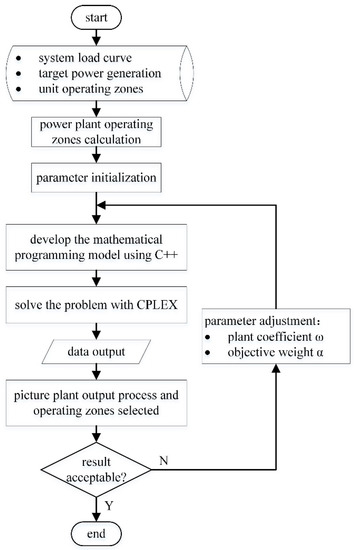
Figure 2.
Model development pipeline.
In the flow chart, the calculation process of power plant operating zones can be briefly described as: set the unit operating zone in the form of a proportion of installed capacity, and then combine the unit operating zones to obtain the final plant-based operating zones. Figure 3 illustrates how the plant-based operating zones can be determined with 1, 2 and 3 units of the same type installed, respectively. In this case, the upper bound of the operating range of an individual unit is its installed capacity while the lower limit is 80% of the installed capacity to ensure the energy conversion efficiency.

Figure 3.
Illustration of the operating zones calculation.
4. Case Studies
4.1. Engineering Background
Yunnan province, located in the far southwest of China, is rich in hydroelectric resources, with an installed hydropower capacity of 67.79 GW at the end of 2019. The total installed capacity under the Yunnan power grid reaches 95.00 GW at the end of 2019, among which 71.36% is hydroelectric. With an installed capacity of 20.61 GW, the Lancang hydropower cascade shares a very large portion of power generation in the Yunnan power grids and plays a crucial role in peak-shaving for the system.
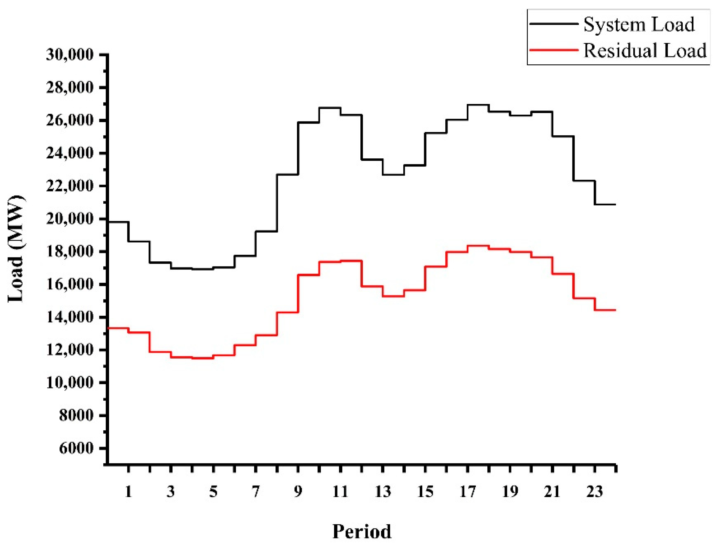
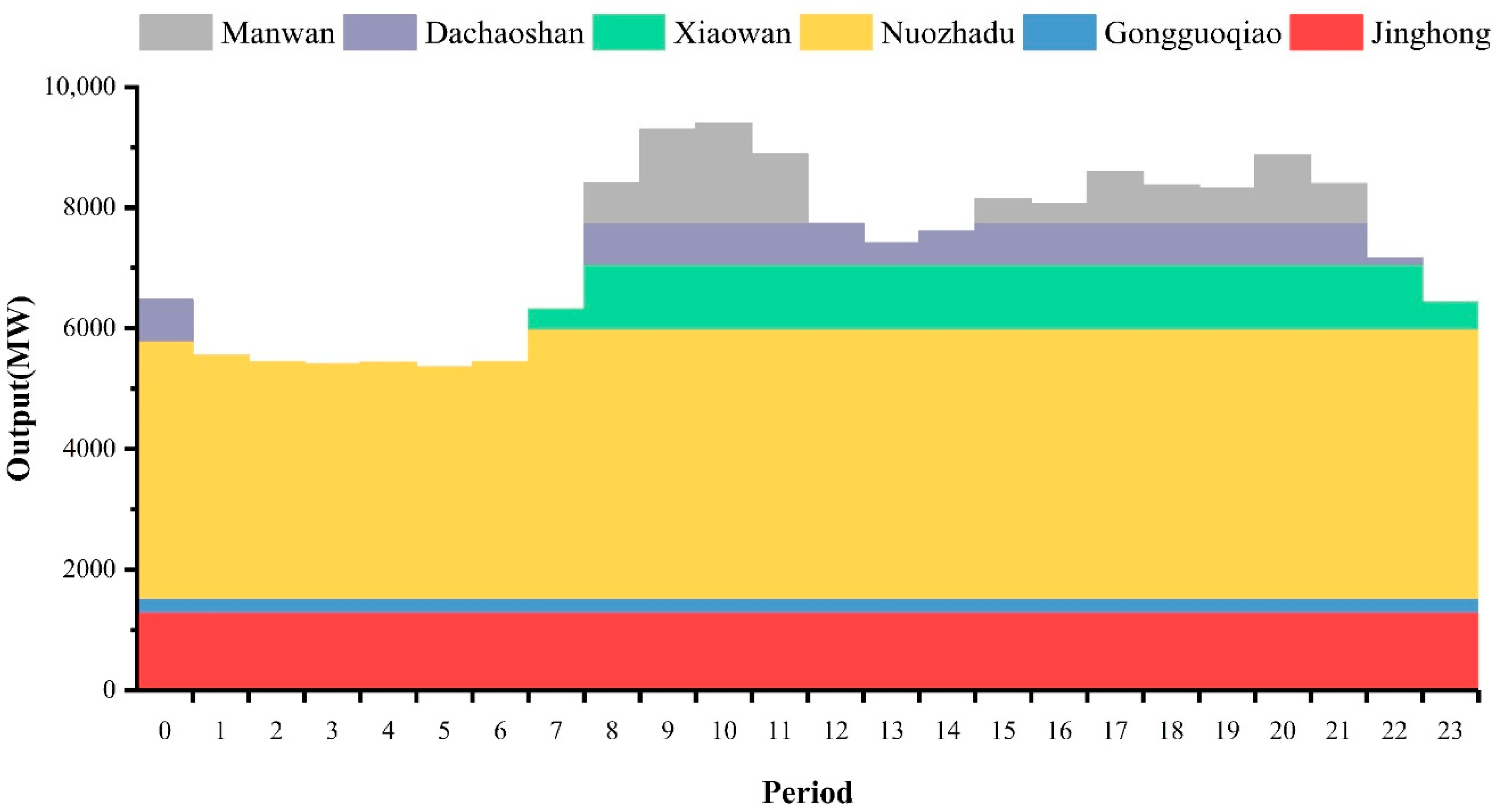
This work selects 6 huge hydropower plants in the middle and lower reaches of the Lancang River, which has a total installed capacity up to about 15.73 GW, accounting for 76% of all the cascade’s installed capacity, and plays a very important role in peak shaving for the Yunnan power grids. The basic characteristics of the selected hydropower stations are given in Table 1. Given 31 April 2018, for instance, the residual load curve with the historical output of the selected plants deducted is compared with the complete load curve of the whole province in Figure 4. For further discussion, the Average Hourly Ramp (AHR) is defined as the average change of output power from an hour period to its next period during the day, and should always be positive whether the power is getting larger or smaller in the next period. Thus, the AHR can be determined for both the provincial load in total and the residual load after deducted by the total power output of the six hydro plants. Taking 31 April 2018 for example, the AHR for the residual load is 737 MW/h, which decreases by 38% compared with the original load, which has an AHR of 1200 MW/h. The observed power generation data of the six plants on 31 April 2018 is taken as the daily generation target in this case study. Figure 5 shows the historical generation process of selected plants in the form of stacking histogram. The MILP model for peak-shaving proposed in this work is applied to rearrange the 24 h scheduling of every power plant with given constraints satisfied.

Table 1.
Basic characteristics of hydropower stations.

Figure 4.
Load curve on 31 April 2018.
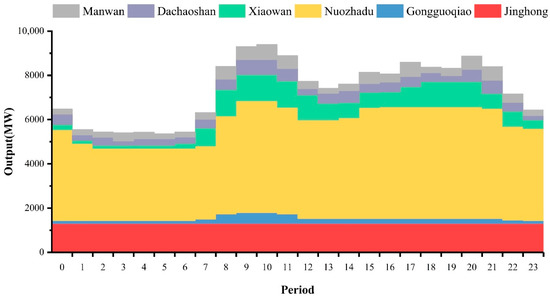
Figure 5.
Historical hourly power generations.
4.2. Parameter Setting
Considering different types of power sources and their regulation performance, Liu, S, et al. [18] classified the power plants into five categories: base, forecasted, minor, and major, as well as peak plants. Among these plants, the base plants represent those under the jurisdiction of dispatching authority and generate firm power output all day. The forecasted plants usually consist of variable wind, solar, and run-of-river hydro plants and will run as forecasted. Plants that have minor operability in peak-shaving loads can be classified into minor plants. The major plants are the ones primarily responsible for the balance of electric power and energy, and the peak plants imply that they are the vital plants to follow the power loads at every time step and always have good performance on regulation. Corresponding to the five categories above, plant coefficients ω can be set as an integer from 1 to 5. Among the six plants selected in this work, Manwan and Dachaoshan generally undertake the main task of peak-shaving regulation and allow a large degree of output fluctuation as well as a slight work capacity violation. Thus, the coefficients of these two plants are set to 1. Nuozhadu and Xiaowan are the backbone plants of the Lancang hydropower cascade with outstanding regulation performance, which allows the two hydro plants to participate in peak-shaving regulation partly, so have their coefficients set as 2. For the remaining plants of the cascade, the value between 3 and 5 is taken according to their plant types.
In the case studies of this work, the weights of each sub-objectives are given in Table 2. Enforcing the transactional energy has a direct impact on the economic benefits and fulfillment ability of the power plant, and is given the highest priority. Limited by the unit characteristics, the power output variation between two adjacent periods should be less than a safe threshold, and the objective of minimizing the output variation should also be given a relatively high priority. The working capacity violation and TVI have not been well studied, playing an auxiliary role in the model and having a lower priority.

Table 2.
Weights of the objective function.
4.3. Results and Discussions
In this study, the model is established using Visual Studio 2015 and solved with the CPLEX12.9.0 optimizer. The final solution time of the case is 4 min and 11 s running in AMD FX-7500 environment. However, for different cases, a reasonable time cannot be guaranteed and it perhaps exceeds 20 min. Figure 6 shows the peak-shaving results in stacking histogram.
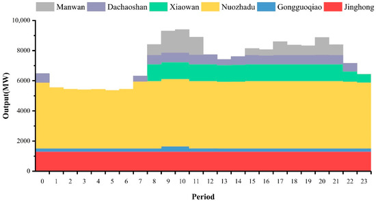
Figure 6.
Hourly power generations of plants (chronologically).
From Figure 6, it can be seen that Manwan operates at the top position, and the peak-shaving effect is significant; Jinghong and Gongguoqiao operate at the baseload position, and their power output during the day is relatively stable. Generally, the results are reasonable and in line with expected. The detailed hourly power outputs are given in Table 3. In particular, sorting the power outputs according to the assumed total loads in ascending order from small to large, the consistency of single plant output process with the trend of the assumed load can be examined, as shown in Figure 7.

Table 3.
Hourly power generations of plants.
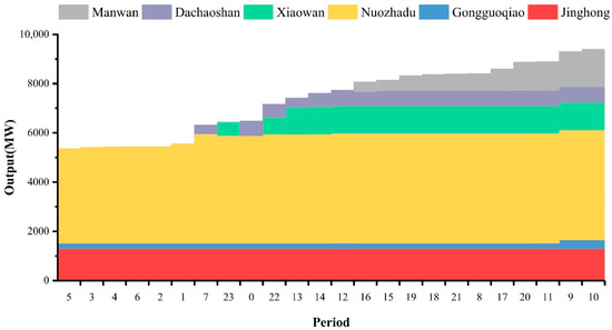
Figure 7.
Hourly power generations of plants (in ascending order of load).
As seen in Figure 7, except that the power output of Jinghong remains unchanged within a day, the trend of the output variation of other power plants is basically consistent with the trend of load, showing that all plants play some role in responding to the change of the load demand. Due to the constraints on operational zones of the power plant, there are some periods where the trend consistency is violated. Figure 8 shows the hourly operating zones of each power plant, where “0” represents the shutdown of all units in the power plant, giving the power output at zero.

Figure 8.
Hourly operating zones of plants.
Particularly for Manwan and Gongguoqiao, Figure 9 and Figure 10 show their hourly power outputs and optimal operational zones, respectively. The results tell that the operational zone of Manwan changes frequently and has a large span. The calculation method of the plant-based operating zones in this work allows Manwan to startup and shut down its units frequently in the operation process so as to achieve a large range of load peak-shaving. Though should have run steadily, Gongguoqiao plant has an operating zone jumping at peak load periods 9 and 10 resulted from the generation target constraint with the highest priority.
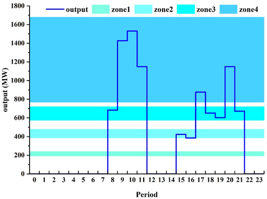
Figure 9.
Hourly power generations and operating zones of Manwan.
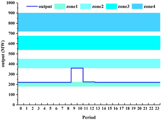
Figure 10.
Hourly power generations and operating zones of Gongguoqiao.
For further discussion, the statistics of AHR on both the plants and cascade are given in Table 4. The AHR of the optimal generation process for individual plants are smaller than the historical data except Manwan, which is classified as a peak plant. The whole cascade’s AHR for the optimized generation is exactly the same as the assumed system load. The results show that the present peak-shaving model performs well on taking advantage of the complementarity among plants in peak-shaving and every single ramp of each plant contributes to the peak-shaving operation.

Table 4.
Statistics of plant average hourly ramp.
As a comparison, Figure 11 shows the results when the model does not consider the constraints of the plant-based operational zones, which means that the lower limit of unit operation zone is set to 0. Figure 11 indicates the direct peak-shaving effects of the model and shows that every plant has its own operation position on the system load curve.
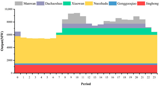
Figure 11.
Hourly power generations of plants (without operating zones enforced).
5. Conclusions
This paper presents a new peak-shaving model based on the MILP to accomplish peak-shaving scheduling, opening up ideas for further in-depth research in the field of power and energy balance. The main contributions of this work include:
- The achievement of the peak-shaving task in an optimization way, showing strength of simplicity in principle and significance in solution efficiency over the traditional peak-shaving method which needs to set the peak-shaving order for each plant;
- A simplified method presented for determining the plant-based operating zones, and the introduction of power output consistency with the trend of system load as constraints that are expressed mathematically;
- The case studies in the Lancang hydropower cascade, suggesting that the model itself has good flexibility, and with further enrichment and expansion, can also be applied to power systems with power plants that can regulate their hourly generations within a day.
Author Contributions
Conceptualization, J.W.; methodology, J.W. and X.C.; software, X.C.; formal analysis, S.F. and Y.H.; data curation, S.F. and Y.H.; Writing—Original draft preparation, X.C.; Writing—Review and editing, J.W.; visualization, X.C., S.F. and Y.H. All authors have read and agreed to the published version of the manuscript.
Funding
This research received no external funding.
Acknowledgments
This research did not receive any specific grant from funding agencies in the public, commercial, or not-for-profit sectors.
Conflicts of Interest
The authors declare no conflict of interest.
References
- Feng, Z.-K.; Niu, W.-J.; Cheng, C.-T.; Zhou, J. Peak shaving operation of hydro-thermal-nuclear plants serving multiple power grids by linear programming. Energy 2017, 135, 210–219. [Google Scholar] [CrossRef]
- Wu, Y. Discussion on key factors for efficient consumption of renewable energy in provincial power grid at southern China. CSEE J. Power Energy Syst. 2020, 6, 554–562. [Google Scholar] [CrossRef]
- Wang, X.; Chang, J.; Meng, X.; Wang, Y. Short-term hydro-thermal-wind-photovoltaic complementary operation of interconnected power systems. Appl. Energy 2018, 229, 945–962. [Google Scholar] [CrossRef]
- Secretariat, R.; Programme, U.E. Renewables 2020 Global Status Report; REN21 Secretariat: Paris, France, 2021; p. 367. [Google Scholar]
- Feng, Z.-K.; Niu, W.-J.; Wang, W.-C.; Zhou, J.-Z.; Cheng, C.-T. A mixed integer linear programming model for unit commitment of thermal plants with peak shaving operation aspect in regional power grid lack of flexible hydropower energy. Energy 2019, 175, 618–629. [Google Scholar] [CrossRef]
- Xie, M.; Zhou, J.; Li, C.; Lu, P. Daily generation scheduling of cascade hydro plants considering peak shaving constraints. J. Water Resour. Plan. Manag. 2016, 142, 11. [Google Scholar] [CrossRef]
- Shen, J.; Cheng, C.-T.; Wang, S.; Yuan, X.; Sun, L.; Zhang, J. Multiobjective optimal operations for an interprovincial hydropower system considering peak-shaving demands. Renew. Sustain. Energy Rev. 2020, 120, 17. [Google Scholar] [CrossRef]
- Gaudard, L.; Romerio-Giudici, F. The future of hydropower in Europe: Interconnecting climate, markets and policies. Environ. Sci. Policy 2014, 37, 172–181. [Google Scholar] [CrossRef]
- Graabak, I.; Korpås, M.; Jaehnert, S.; Belsnes, M. Balancing future variable wind and solar power production in Central-West Europe with Norwegian hydropower. Energy 2019, 168, 870–882. [Google Scholar] [CrossRef]
- Simopoulos, D.N.; Kavatza, S.D.; Vournas, C.D. An enhanced peak shaving method for short term hydrothermal scheduling. Energy Convers. Manag. 2007, 48, 3018–3024. [Google Scholar] [CrossRef]
- Wu, R.N.; Lee, T.H.; Hill, E.F. An investigation of the accuracy and the characteristics of the peak-shaving method applied to production cost calculations. IEEE Trans. Power Syst. 1989, 4, 1043–1049. [Google Scholar] [CrossRef]
- Wang, J.; Zhang, Y. Short-term optimal operation of hydropower reservoirs with unit commitment and navigation. J. Water Resour. Plan. Manag. 2012, 138, 3–12. [Google Scholar] [CrossRef]
- Wu, X.; Cheng, C.-T.; Shen, J.-J.; Luo, B.; Liao, S.; Li, G. A multi-objective short term hydropower scheduling model for peak shaving. Int. J. Electr. Power Energy Syst. 2015, 68, 278–293. [Google Scholar] [CrossRef]
- Wang, J.; Liu, S.; Zhang, Y. Quarter-hourly operation of large-scale hydropower reservoir systems with prioritized constraints. J. Water Resour. Plan. Manag. 2015, 141, 13. [Google Scholar] [CrossRef]
- Chang, G.W.; Tsai, Y.D.; Lai, C.Y.; Chung, J.S. A practical mixed integer linear programming based approach for unit commitment. In Proceedings of the IEEE Power Engineering Society General Meeting, Denver, CO, USA, 6–10 June 2004; Volume 221, pp. 221–225. [Google Scholar]
- Tong, B.; Zhai, Q.; Guan, X. An MILP based formulation for short-term hydro generation scheduling with analysis of the linearization effects on solution feasibility. IEEE Trans. Power Syst. 2013, 28, 3588–3599. [Google Scholar] [CrossRef]
- Ma, T.; Wang, J.; Liu, Y.; Sun, H.; Gui, D.; Xue, J. A mixed integer linear programming method for optimizing layout of irrigated pumping well in oasis. Water 2019, 11, 1185. [Google Scholar] [CrossRef]
- Liu, S.; Xie, M. Modeling the daily generation schedules in under-developed electricity markets with high-share renewables: A case study of Yunnan in China. Energy 2020, 201, 117677. [Google Scholar] [CrossRef]
Publisher’s Note: MDPI stays neutral with regard to jurisdictional claims in published maps and institutional affiliations. |
© 2021 by the authors. Licensee MDPI, Basel, Switzerland. This article is an open access article distributed under the terms and conditions of the Creative Commons Attribution (CC BY) license (http://creativecommons.org/licenses/by/4.0/).

