An Efficient Backward/Forward Sweep Algorithm for Power Flow Analysis through a Novel Tree-Like Structure for Unbalanced Distribution Networks

Abstract

The increase of distributed energy resources (DERs) in low voltage (LV) distribution networks requires the ability to perform an accurate power flow analysis (PFA) in unbalanced systems. The characteristics of a well performing power flow algorithm are the production of accurate results, robustness and quick convergence. The current study proposes an improvement to an already used backward-forward sweep (BFS) power flow algorithm for unbalanced three-phase distribution networks. The proposed power flow algorithm can be implemented in large systems producing accurate results in a small amount of time using as little computational resources as possible. In this version of the algorithm, the network is represented in a tree-like structure, instead of an incidence matrix, avoiding the use of redundant computations and the storing of unnecessary data. An implementation of the method was developed in Python programming language and tested for 3 IEEE feeder test cases (the 4 bus feeder, the 13 bus feeder and the European Low Voltage test feeder), ranging from a low (4) to a very high (907) buses number, while including a wide variety of components witnessed in LV distribution networks.

1. Introduction

In order to properly control and protect a power system, its state must be known so that appropriate actions are taken. Its state is defined as the magnitude and phase of the phase voltages of each bus. The state of the power system is determined through a power flow analysis (PFA). However, the method through which the PFA is performed depends on whether it is applied at the transmission or distribution level of the system. Specifically, the standard Newton-Raphson Algorithm used for PFA of transmission systems cannot be used in many cases on distribution systems due to their topology [1]. Thus, a lot of research has focused on modelling distribution systems and their components for use in PFA. Such research is necessary as distribution networks present characteristics that differ from those of transmission networks. These characteristics include the presence of distributed generation, which is used increasingly due to its lower environmental impact, a radial network structure, single phase or unbalanced consumer loads and high resistance to reactance ratio on lines [1]. Because of the single phase or unbalanced loads, the standard PFA, that assumes a balanced network, is insufficient. In addition to the imbalances present, the number of iterations and convergence of PFA is further affected by the characteristics of the distribution network to be studied, the method used to construct and solve the system equations, as well as the reference frame and transformer model used. A way to tackle this problem is to take advantage of the radial structure of distribution networks through a backward-forward sweep (BFS). It involves separating the original system of equations, into two separate systems and solving one, using the last results of the other, until convergence is achieved. Solving for the currents with the voltages given is called the backward sweep (BS) and solving for the voltages with the currents given is called the forward sweep (FS). Of note, BFS can only be used in radial networks, but if the network is indeed radial, as is often the case [2,3], distributed generation like solar panels can be modelled using components presented in this paper, like power-voltage or PQ generators.

A BFS is utilized in [4,5], along with an abc reference frame, which may cause a failure to converge when multiple transformer connections are present [6], while [7] uses BFS along with an admittance matrix to formulate the problem, but in case any system component is altered this matrix must be rebuilt, raising the complexity.

Of note, an improved BFS approach is demonstrated in [8,9], where instead of complex voltages, their real and imaginary parts are calculated instead and then added again to return to complex form. However, it involves solving the circuits twice (both real and imaginary) unlike in the presented method, which only requires solving one circuit in the optimal way. Finally, a dq0 reference frame was implemented in [10], but did not include transformer modelling, and in [11], where Jacobian matrices that increased complexity were used.

Traditional approaches with Jacobian matrices are presented in [12,13,14,15], while [16] takes advantage of linear approximations to simplify the Jacobians. References [17,18] use Jacobians in the three sequence networks of an unbalanced network. All these approaches, while effective, require an increased number of computations due to the many matrix operations involved.

Linear approximations are also the basis for [19,20], but these approximation techniques can lack in accuracy or convergence speed in comparison to the BFS algorithms.

The most thorough method for PFA on unbalanced power systems has been presented in [21,22,23]. It includes the use of a BFS, in combination with the αβ0 reference frame, which allows modelling both transformers and regulators in a new and unified way similar to transmission lines. The linear system equations are expressed using the node incidence matrix instead of the admittance matrix of the power system. The equations can then be solved using different methods. Furthermore, different load and generators models can be added to the core linear equations depending on the application. For example, the authors of the three afore-mentioned papers chose a trust-region-dopleg algorithm as presented in [24]. The features of this PFA version ensure convergence, even if the initial voltage profile estimate is not optimal. The only problem presented is when PFA is required for large power systems. In these cases, the running time and memory usage are extremely high and render the PFA ineffective. The prohibitive running time and memory usage are the result of very large systems of equations, represented as matrices, which must be solved many times each, to achieve convergence.

The present work adopts the transformer modelling and the BFS approaches presented in [21,22,23] and improves them in terms of running time and memory requirements. In particular, it modifies the BFS to solve the tree formed by the distribution network, level by level, which leads to accurate results within very short running times and low memory usage, even in systems with a large number of buses. Though the algorithm has been developed in Python, this modification can be used in any programming language and as such is extremely useful. Implementations of the standard and the proposed method are developed and tested in networks of various sizes (smaller network with 4 buses, the largest one with 907 buses), that include a large variety of components that are witnessed in low voltage (LV) distribution systems. The two implementations produce the same accurate results. The largest error observed was 5 × 10⁻². The purpose of testing is to compare the runtime of both methods, witnessing great improvement in large systems. The short running time resulting from the algorithm modification allows problems, like tap optimization, which are difficult to solve efficiently from a computational perspective, to be studied with an exhaustive search of all possible combinations.

In conclusion, the paper’s main goal is to optimize the BFS approach to solving power flows to the highest possible degree, both in terms of running time and memory usage. The next sections are devoted to the description of the proposed methodology, the presentation of the corresponding results and the elicitation of useful conclusions. In particular, the second section of the paper presents the modelling used for all components included in the power systems under study and the proposed algorithm including the pseudocode, the third one presents the standard and proposed methods’ results regarding running time and memory requirements along with a comparison between them, while in the fourth section the results are discussed and conclusions are drawn. Finally, a Nomenclature section explaining the numerous symbols and subscripts found in Section 2 is included before the References section to facilitate the readability and comprehension of the equations presented.

2. Materials and Methods

In order for the PFA equations to be formulated, components of the power system such as generators, loads, transformers, regulators and distribution lines must be properly modelled.

2.1. Per-Unit System Bases

The per-unit system is used for the algorithm as it greatly simplifies power system analysis and allows for a common iterations termination criterion for all power systems.

First, a base power ${\mathrm{S}}_{\mathrm{base}}$ (per phase) is selected for the whole power system. The base power is equal to the greatest rated power among the components of the power system under study, divided by 3.

Then, a base voltage ${\mathrm{V}}_{\mathrm{base}}$ is selected for each section of the power system with a different voltage level. This means that n + 1 base voltages are selected, if a power system has n transformers. A base voltage of a section can be equal to the base voltage of a different section of the power system. Each base voltage is equal to the rated voltage of the respective transformer side, divided by $\sqrt{3}$ (phase voltage).

Using the base power ${\mathrm{S}}_{\mathrm{base}}$ of the system and the base voltages ${\mathrm{V}}_{\mathrm{base}}$ of each section defined by the transformers, the other base quantities for each section can be calculated by:

$${\mathrm{I}}_{\mathrm{base}}=\frac{{\mathrm{S}}_{\mathrm{base}}}{{\mathrm{V}}_{\mathrm{base}}}$$

(1)

$${\mathrm{Z}}_{\mathrm{base}}=\frac{{\mathrm{V}}_{\mathrm{base}}^2}{{\mathrm{S}}_{\mathrm{base}}}$$

(2)

These per-unit quantities are used for all equations in the following sections of this report. A per-unit quantity can be reverted to its normal value by multiplying it with its base. Many power system components, such as transformers, specify their impedance in the per-unit system, using their rated power and voltage as bases. If the base power ${\mathrm{S}}_{\mathrm{base},\mathrm{rated}}$ or base voltage ${\mathrm{V}}_{\mathrm{base},\mathrm{rated}}$ of a component differs from the base power of the power system ${\mathrm{S}}_{\mathrm{base},\mathrm{system}}$ or the base voltage ${\mathrm{V}}_{\mathrm{base},\mathrm{new}}$ chosen for its section of the power system, its appropriate per-unit impedance for the given section can be calculated by:

$${\overline{\mathrm{Z}}}_{\mathrm{pu},\mathrm{new}}=\frac{{\mathrm{S}}_{\mathrm{base},\mathrm{system}}}{{\mathrm{S}}_{\mathrm{base},\mathrm{rated}}}\times \frac{{\mathrm{V}}_{\mathrm{base},\mathrm{rated}}^2}{{\mathrm{V}}_{\mathrm{base},\mathrm{section}}^2}\times {\overline{\mathrm{Z}}}_{\mathrm{pu},\mathrm{rated}}$$

(3)

2.2. αβ0 System

Each voltage, power and current in an unbalanced power system with three phases is a 3 × 1 vector, where each vector element corresponds to one phase. For example, the voltage of bus i ${\overline{\mathbf{V}}}_{\mathbf{i}}$ is:

$${\overline{\mathbf{V}}}_{\mathbf{i}}=\left[\begin{array}{c}{\overline{\mathrm{V}}}_{\mathrm{i},\mathrm{a}}\\ {\overline{\mathrm{V}}}_{\mathrm{i},\mathrm{b}}\\ {\overline{\mathrm{V}}}_{\mathrm{i},\mathrm{c}}\end{array}\right]$$

(4)

In order to ensure convergence of the PFA [21] and further simplify its equations, the αβ0 system is used alongside the per-unit system, instead of the abc system. If a 3 × 1 vector $\overline{\mathbf{vector}}$ is given in the abc system, it can be converted to the 3 × 1 αβ0 system vector ${\overline{\mathbf{vector}}}^{\mathsf{\alpha }\mathsf{\beta }\mathbf{0}}$ by:

$${\overline{\mathbf{vector}}}^{\mathsf{\alpha }\mathsf{\beta }\mathbf{0}}{=\mathbf{A}}^{-\mathbf{1}}\times \overline{\mathbf{vector}}$$

(5)

where:

$$\mathbf{A}=\left[\begin{array}{ccc}\frac{\sqrt{2}}{\sqrt{3}}& 0& \frac{1}{\sqrt{3}}\\ -\frac{1}{\sqrt{6}}& \frac{1}{\sqrt{2}}& \frac{1}{\sqrt{2}}\\ -\frac{1}{\sqrt{6}}& -\frac{1}{\sqrt{2}}& \frac{1}{\sqrt{2}}\end{array}\right]$$

(6)

and $\mathbf{A}$ has the useful property:

$${\mathbf{A}}^{-\mathbf{1}}{=\mathbf{A}}^{\mathbf{T}}$$

(7)

Thus, (5) becomes:

$${\overline{\mathbf{vector}}}^{\mathsf{\alpha }\mathsf{\beta }\mathbf{0}}{=\mathbf{A}}^{\mathbf{T}}\times \overline{\mathbf{vector}}$$

(8)

Similarly, a 3 × 1 vector in the αβ0 system ${\overline{\mathbf{vector}}}^{\mathsf{\alpha }\mathsf{\beta }\mathbf{0}}$ can be converted to the 3 × 1 abc system vector $\overline{\mathbf{vector}}$ by:

$$\overline{\mathbf{vector}}=\mathbf{A}\times {\overline{\mathbf{vector}}}^{\mathsf{\alpha }\mathsf{\beta }\mathbf{0}}$$

(9)

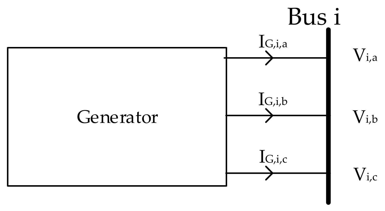
2.3. Generators, Loads and Buses

There are 2 types of generators (a generator at bus i is shown in Figure 1) depending on the control technique applied on them: Power-Voltage (PV) generators and PQ generators.

Loads (a load at bus i is shown in Figure 2) represent customer consumption, capacitor banks or distributed generation and are connected in Y_g or Δ configuration. There are three types of loads: PQ loads, I loads, Z loads [25]. For example, data centers, electric vehicles or DC motors are usually represented as PQ loads, street lighting and renewable energy sources are usually represented as I loads. Resistance heating loads and parasitic impedances of distribution are usually represented as Z loads.

Buses are the nodes of the power system. There are 3 types of buses i.e., Slack, PV, and PQ ones.

A bus with known voltage magnitude and angle is a slack bus that is described by:

$${\overline{\mathbf{V}}}_{\mathbf{i}}=\left[\begin{array}{c}{\overline{\mathrm{V}}}_{\mathrm{i},\mathrm{a}}\\ {\overline{\mathrm{V}}}_{\mathrm{i},\mathrm{b}}\\ {\overline{\mathrm{V}}}_{\mathrm{i},\mathrm{c}}\end{array}\right] \mathrm{remains} \mathrm{constant}$$

(10)

Usually the angles of phases a, b, c of the slack bus are 0 degrees (reference), −120 degrees and 120 degrees respectively.

PQ generators generate constant complex power and are described by:

$${\overline{\mathbf{S}}}_{\mathbf{G},\mathbf{i}}=\left[\begin{array}{c}{\overline{\mathrm{S}}}_{\mathrm{G},\mathrm{i},\mathrm{a}}\\ {\overline{\mathrm{S}}}_{\mathrm{G},\mathrm{i},\mathrm{b}}\\ {\overline{\mathrm{S}}}_{\mathrm{G},\mathrm{i},\mathrm{c}}\end{array}\right]=\left[\begin{array}{c}{\overline{\mathrm{V}}}_{\mathrm{i},\mathrm{a}}\times \mathrm{conj}({\overline{\mathrm{I}}}_{\mathrm{G},\mathrm{i},\mathrm{a}})\\ {\overline{\mathrm{V}}}_{\mathrm{i},\mathrm{b}}\times \mathrm{conj}({\overline{\mathrm{I}}}_{\mathrm{G},\mathrm{i},\mathrm{b}})\\ {\overline{\mathrm{V}}}_{\mathrm{i},\mathrm{c}}\times \mathrm{conj}({\overline{\mathrm{I}}}_{\mathrm{G},\mathrm{i},\mathrm{c}})\end{array}\right]\mathrm{remains} \mathrm{constant}$$

(11)

where ${\overline{\mathrm{S}}}_{\mathrm{G},\mathrm{i},\mathrm{ph}}$ and ${\overline{\mathrm{I}}}_{\mathrm{G},\mathrm{i},\mathrm{ph}}$ are the generated power and current at each phase, ph$\in \left\{\mathrm{a},\mathrm{b},\mathrm{c}\right\}$ of bus i, respectively.

Power-Voltage generators have constant voltage magnitude, generate constant real power and are described by:

$$\mathrm{abs}({\overline{\mathbf{V}}}_{\mathbf{i}})=\left[\begin{array}{c}\mathrm{abs}({\overline{\mathrm{V}}}_{\mathrm{i},\mathrm{a}})\\ \mathrm{abs}({\overline{\mathrm{V}}}_{\mathrm{i},\mathrm{b}})\\ \mathrm{abs}({\overline{\mathrm{V}}}_{\mathrm{i},\mathrm{c}})\end{array}\right] \mathrm{remains} \mathrm{constant}$$

(12)

$$\mathrm{re}\left({\overline{\mathbf{S}}}_{\mathbf{G},\mathbf{i}}\right)=\left[\begin{array}{c}\mathrm{Re}({\overline{\mathrm{S}}}_{\mathrm{G},\mathrm{i},\mathrm{a}})\\ \mathrm{Re}({\overline{\mathrm{S}}}_{\mathrm{G},\mathrm{i},\mathrm{b}})\\ \mathrm{Re}({\overline{\mathrm{S}}}_{\mathrm{G},\mathrm{i},\mathrm{c}})\end{array}\right] \mathrm{remains} \mathrm{constant}$$

(13)

For all loads, their complex power consumption is given by:

$${\overline{\mathbf{S}}}_{\mathbf{L},\mathbf{i}}=\left[\begin{array}{c}{\overline{\mathrm{S}}}_{\mathrm{L},\mathrm{i},\mathrm{a}}\\ {\overline{\mathrm{S}}}_{\mathrm{L},\mathrm{i},\mathrm{b}}\\ {\overline{\mathrm{S}}}_{\mathrm{L},\mathrm{i},\mathrm{c}}\end{array}\right]=\left[\begin{array}{c}{\overline{\mathrm{V}}}_{\mathrm{i},\mathrm{a}}\times \mathrm{conj}({\overline{\mathrm{I}}}_{\mathrm{L},\mathrm{i},\mathrm{a}})\\ {\overline{\mathrm{V}}}_{\mathrm{i},\mathrm{b}}\times \mathrm{conj}({\overline{\mathrm{I}}}_{\mathrm{L},\mathrm{i},\mathrm{b}})\\ {\overline{\mathrm{V}}}_{\mathrm{i},\mathrm{c}}\times \mathrm{conj}({\overline{\mathrm{I}}}_{\mathrm{L},\mathrm{i},\mathrm{c}})\end{array}\right]$$

(14)

and their voltage drop is given by Ohm’s Law:

$${\overline{\mathbf{V}}}_{\mathbf{L},\mathbf{i}}=\left[\begin{array}{c}{\overline{\mathrm{V}}}_{\mathrm{L},\mathrm{i},\mathrm{a}}\\ {\overline{\mathrm{V}}}_{\mathrm{L},\mathrm{i},\mathrm{b}}\\ {\overline{\mathrm{V}}}_{\mathrm{L},\mathrm{i},\mathrm{c}}\end{array}\right]=\left[\begin{array}{c}{\overline{\mathrm{Z}}}_{\mathrm{L},\mathrm{i},\mathrm{a}}\times {\overline{\mathrm{I}}}_{\mathrm{L},\mathrm{i},\mathrm{a}}\\ {\overline{\mathrm{Z}}}_{\mathrm{L},\mathrm{i},\mathrm{b}}\times {\overline{\mathrm{I}}}_{\mathrm{L},\mathrm{i},\mathrm{b}}\\ {\overline{\mathrm{Z}}}_{\mathrm{L},\mathrm{i},\mathrm{c}}\times {\overline{\mathrm{I}}}_{\mathrm{L},\mathrm{i},\mathrm{c}}\end{array}\right]$$

(15)

where ${\overline{\mathrm{S}}}_{\mathrm{L},\mathrm{i},\mathrm{ph}}$ and ${\overline{\mathrm{I}}}_{\mathrm{L},\mathrm{i},\mathrm{ph}}$ are the consumed power and current of the load at each phase ph$\in \left\{\mathrm{a},\mathrm{b},\mathrm{c}\right\}$ of bus i, respectively and ${\overline{\mathrm{Z}}}_{\mathrm{L},\mathrm{i},\mathrm{ph}}$ is the impedance of the load at phase ph$\in \left\{\mathrm{a},\mathrm{b},\mathrm{c}\right\}$ of bus i.

PQ loads consume constant complex power and are described by:

$${\overline{\mathbf{S}}}_{\mathbf{L},\mathbf{i}}=\left[\begin{array}{c}{\overline{\mathrm{S}}}_{\mathrm{L},\mathrm{i},\mathrm{a}}\\ {\overline{\mathrm{S}}}_{\mathrm{L},\mathrm{i},\mathrm{b}}\\ {\overline{\mathrm{S}}}_{\mathrm{L},\mathrm{i},\mathrm{c}}\end{array}\right]=\left[\begin{array}{c}{\overline{\mathrm{V}}}_{\mathrm{i},\mathrm{a}}\times \mathrm{conj}({\overline{\mathrm{I}}}_{\mathrm{L},\mathrm{i},\mathrm{a}})\\ {\overline{\mathrm{V}}}_{\mathrm{i},\mathrm{b}}\times \mathrm{conj}({\overline{\mathrm{I}}}_{\mathrm{L},\mathrm{i},\mathrm{b}})\\ {\overline{\mathrm{V}}}_{\mathrm{i},\mathrm{c}}\times \mathrm{conj}({\overline{\mathrm{I}}}_{\mathrm{L},\mathrm{i},\mathrm{c}})\end{array}\right] \mathrm{remains} \mathrm{constant}$$

(16)

I loads have a constant current magnitude and a constant power factor and are described by:

$$\mathrm{abs}({\overline{\mathbf{I}}}_{\mathbf{L},\mathbf{i}})=\left[\begin{array}{c}\mathrm{abs}({\overline{\mathrm{I}}}_{\mathrm{L},\mathrm{i},\mathrm{a}})\\ \mathrm{abs}({\overline{\mathrm{I}}}_{\mathrm{L},\mathrm{i},\mathrm{b}})\\ \mathrm{abs}({\overline{\mathrm{I}}}_{\mathrm{L},\mathrm{i},\mathrm{c}})\end{array}\right] \mathrm{remains} \mathrm{constant}$$

(17)

$$\arg \left({\overline{\mathbf{S}}}_{\mathbf{L},\mathbf{i}}\right)=\left[\begin{array}{c}\arg ({\overline{\mathrm{S}}}_{\mathrm{L},\mathrm{i},\mathrm{a}})\\ \arg ({\overline{\mathrm{S}}}_{\mathrm{L},\mathrm{i},\mathrm{b}})\\ \arg ({\overline{\mathrm{S}}}_{\mathrm{L},\mathrm{i},\mathrm{c}})\end{array}\right] \mathrm{remains} \mathrm{constant}$$

(18)

Z Loads have constant impedance and are described by:

$${\overline{\mathbf{Z}}}_{\mathbf{L},\mathbf{i}}=\left[\begin{array}{c}{\overline{\mathrm{Z}}}_{\mathrm{i},\mathrm{a}}\\ {\overline{\mathrm{Z}}}_{\mathrm{i},\mathrm{b}}\\ {\overline{\mathrm{Z}}}_{\mathrm{i},\mathrm{c}}\end{array}\right] \mathrm{remains} \mathrm{constant}$$

(19)

Equations (14)–(19) refer to star-connected loads. In the case of delta-connected loads, the subscripts a, b, c are replaced by the subscripts ab, bc and ca, respectively.

2.4. Transformers

Transformers (a transformer at bus i is shown in Figure 3) are not ideal and have losses, which are modelled as an impedance $\overline{\mathrm{Z}}$ equal to:

$$\overline{\mathbf{Z}}=\overline{\mathrm{Z}}\times \left[\begin{array}{ccc}1& 0& 0\\ 0& 1& 0\\ 0& 0& 1\end{array}\right]=\overline{\mathrm{Z}}\times \mathbf{Id}=(\mathrm{R}+\mathrm{j}\times \mathrm{X})\times \mathbf{Id}$$

(20)

where Id is the 3 × 3 identity matrix and R and X are the phase resistance and reactance, respectively.

Primary current ${\overline{\mathbf{I}}}_{\mathbf{P}}$ is defined as ${\overline{\mathbf{I}}}_{\mathbf{ij}}$ and secondary current ${\overline{\mathbf{I}}}_{\mathbf{s}}$ is defined as ${\overline{\mathbf{I}}}_{\mathbf{ji}}$. Depending on the transformer connection, different equations are used to relate the primary and secondary voltages with the primary and secondary currents. These equations are given in [21].

2.5. Regulators

Only ideal regulators (a regulator at bus i is shown in Figure 4) with zero impedance and configuration Yg-Yg are considered, as only those are used for the IEEE networks under study. The factor r is a given real constant of each regulator that depends on how the windings of the transformer are connected (step-up or step-down) and their turns.

The equations defining the operation of a regulator with known r for the PFA are [23]:

$${\overline{\mathbf{V}}}_{\mathbf{l}-\mathbf{n},\mathbf{P}}^{\mathsf{\alpha }\mathsf{\beta }0}{=\mathbf{N}}_{\mathbf{1}}\times {\overline{\mathbf{V}}}_{\mathbf{l}-\mathbf{n},\mathbf{S}}^{\mathsf{\alpha }\mathsf{\beta }\mathbf{0}}+{\mathbf{N}}_{\mathbf{2}}\times {\overline{\mathbf{I}}}_{\mathbf{P}}^{\mathsf{\alpha }\mathsf{\beta }0}$$

(21)

where the subscript l−n denotes line-to-neutral voltages and:

$${\mathbf{N}}_{\mathbf{1}}{=\mathbf{A}}^{-\mathbf{1}}\times \left[\begin{array}{ccc}\mathrm{r}& 0& 0\\ 0& \mathrm{r}& 0\\ 0& 0& \mathrm{r}\end{array}\right]\times \mathbf{A}$$

(22)

$${\mathbf{N}}_{\mathbf{2}}=\mathbf{0}$$

(23)

For the regulator currents:

$${\mathbf{0}=\mathbf{N}}_{\mathbf{3}}\times {\overline{\mathbf{I}}}_{\mathbf{P}}^{\mathsf{\alpha }\mathsf{\beta }\mathbf{0}}+{\mathbf{N}}_{\mathbf{4}}\times {\overline{\mathbf{I}}}_{\mathbf{S}}^{\mathsf{\alpha }\mathsf{\beta }\mathbf{0}}$$

(24)

where:

$${\mathbf{N}}_{\mathbf{3}}{=-\mathbf{A}}^{-\mathbf{1}}\times \left[\begin{array}{ccc}\mathrm{r}& 0& 0\\ 0& \mathrm{r}& 0\\ 0& 0& \mathrm{r}\end{array}\right]\times \mathbf{A}$$

(25)

$${\mathbf{N}}_{\mathbf{4}}=-\mathbf{Id}$$

(26)

where Id is the 3 $\times$ 3 identity matrix.

2.6. Distribution Lines

Electric power is distributed to the loads through distribution lines (a distribution line between bus i and bus j is shown in Figure 5). Distribution lines are made up of three phase conductors a, b, c and in some cases a neutral conductor. Aside from the voltage drop of each conductor, due to its own current, each conductor also has a voltage drop associated with the current of all other conductors present, due to mutual conductance.

The voltage drop of each phase can be determined as a function of the current of each phase:

$$\left[\begin{array}{c}{\overline{\mathrm{V}}}_{\mathrm{i},\mathrm{a}}\\ {\overline{\mathrm{V}}}_{\mathrm{i},\mathrm{b}}\\ {\overline{\mathrm{V}}}_{\mathrm{i},\mathrm{c}}\end{array}\right]=\left[\begin{array}{c}{\overline{\mathrm{V}}}_{\mathrm{j},\mathrm{a}}\\ {\overline{\mathrm{V}}}_{\mathrm{j},\mathrm{b}}\\ {\overline{\mathrm{V}}}_{\mathrm{j},\mathrm{c}}\end{array}\right]+{\overline{\mathbf{Z}}}_{\mathbf{ij}}\times \left[\begin{array}{c}{\overline{\mathrm{I}}}_{\mathrm{ij},\mathrm{a}}\\ {\overline{\mathrm{I}}}_{\mathrm{ij},\mathrm{b}}\\ {\overline{\mathrm{I}}}_{\mathrm{ij},\mathrm{c}}\end{array}\right]$$

(27)

where ${\overline{\mathbf{Z}}}_{\mathbf{ij}}$ is the 6 × 6 impedance matrix of the distribution line.

Multiplying from the left with ${\mathbf{A}}^{-\mathbf{1}}$ and then from the right with $\mathbf{A}$ converts (27) into the αβ0 system:

$${\overline{\mathbf{V}}}_{\mathbf{l}-\mathbf{n},\mathbf{i}}^{\mathsf{\alpha }\mathsf{\beta }\mathbf{0}}={\mathbf{N}}_{\mathbf{1}}\times {\overline{\mathbf{V}}}_{\mathbf{l}-\mathbf{n},\mathbf{j}}^{\mathsf{\alpha }\mathsf{\beta }\mathbf{0}}+{\mathbf{N}}_{\mathbf{2}}\times {\overline{\mathbf{I}}}_{\mathbf{ij}}^{\mathsf{\alpha }\mathsf{\beta }\mathbf{0}}$$

(28)

where:

$${\mathbf{N}}_{\mathbf{1}}=\mathbf{Id}$$

(29)

$${\mathbf{N}}_{\mathbf{2}}{=\mathbf{A}}^{-\mathbf{1}}\times {\overline{\mathbf{Z}}}_{\mathbf{ij}}\times \mathbf{A}$$

(30)

Because line-to-line voltages ${\overline{\mathbf{V}}}_{\mathbf{l}-\mathbf{l}}$ can be derived from line-to-neutral voltages ${\overline{\mathbf{V}}}_{\mathbf{l}-\mathbf{n}}$ through:

$${\overline{\mathbf{V}}}_{\mathbf{l}-\mathbf{l}}=\left[\begin{array}{ccc}1& -1& 0\\ 0& 1& -1\\ -1& 0& 1\end{array}\right]\times {\overline{\mathbf{V}}}_{\mathbf{l}-\mathbf{n}}$$

(31)

then:

$${\overline{\mathbf{V}}}_{\mathbf{l}-\mathbf{l},\mathbf{i}}^{\mathsf{\alpha }\mathsf{\beta }\mathbf{0}}={\mathbf{N}}_{\mathbf{1}}\times {\overline{\mathbf{V}}}_{\mathbf{l}-\mathbf{l},\mathbf{j}}^{\mathsf{\alpha }\mathsf{\beta }\mathbf{0}}+{\mathbf{N}}_{\mathbf{2}}\times {\overline{\mathbf{I}}}_{\mathbf{ij}}^{\mathsf{\alpha }\mathsf{\beta }\mathbf{0}}$$

(32)

where:

$$N_{\mathbf{1}}=Id$$

(33)

$${\mathbf{N}}_{\mathbf{2}}{=\mathbf{A}}^{-\mathbf{1}}\times \left[\begin{array}{ccc}1& -1& 0\\ 0& 1& -1\\ -1& 0& 1\end{array}\right]\times {\overline{\mathbf{Z}}}_{\mathbf{ij}}\times \mathbf{A}$$

(34)

For the distribution line currents:

$$\mathbf{0}={\mathbf{N}}_{\mathbf{3}}\times {\overline{\mathbf{I}}}_{\mathbf{ij}}^{\mathsf{\alpha }\mathsf{\beta }\mathbf{0}}+{\mathbf{N}}_{\mathbf{4}}\times {\overline{\mathbf{I}}}_{\mathbf{ji}}^{\mathsf{\alpha }\mathsf{\beta }\mathbf{0}}$$

(35)

where:

$${\mathbf{N}}_{\mathbf{3}}=\mathbf{Id}$$

(36)

$${\mathbf{N}}_{\mathbf{4}}=\mathbf{Id}$$

(37)

Additional impedances between phases and between phases and ground can be easily included as Z loads.

2.7. Conversion from 3 to 6 Dimensions

After the equations of transformers, regulators and distribution lines are developed, equations of the form:

$$\left[\begin{array}{c}{\overline{\mathrm{a}}}_{\mathsf{\alpha }}\\ {\overline{\mathrm{a}}}_{\mathsf{\beta }}\\ {\overline{\mathrm{a}}}_0\end{array}\right]=\overline{\mathbf{B}}\times \left[\begin{array}{c}{\overline{\mathrm{c}}}_{\mathsf{\alpha }}\\ {\overline{\mathrm{c}}}_{\mathsf{\beta }}\\ {\overline{\mathrm{c}}}_0\end{array}\right]+\overline{\mathbf{D}}\times \left[\begin{array}{c}{\overline{\mathrm{e}}}_{\mathsf{\alpha }}\\ {\overline{\mathrm{e}}}_{\mathsf{\beta }}\\ {\overline{\mathrm{e}}}_0\end{array}\right]$$

namely Equations (21), (24), (28), (32), (35) and the transformer equations are written in the form:

$$\left[\begin{array}{c}\begin{array}{c}\mathrm{Re}({\overline{\mathrm{a}}}_{\mathsf{\alpha }})\\ \mathrm{Re}({\overline{\mathrm{a}}}_{\mathsf{\beta }})\\ \mathrm{Re}({\overline{\mathrm{a}}}_0)\end{array}\\ \begin{array}{c}\mathrm{Im}({\overline{\mathrm{a}}}_{\mathsf{\alpha }})\\ \mathrm{Im}({\overline{\mathrm{a}}}_{\mathsf{\beta }})\\ \mathrm{Im}({\overline{\mathrm{a}}}_0)\end{array}\end{array}\right]=\left[\begin{array}{cc}\mathrm{Re}(\overline{\mathbf{B}})& -\mathrm{Im}(\overline{\mathbf{B}})\\ \mathrm{Im}(\overline{\mathbf{B}})& \mathrm{Re}(\overline{\mathbf{B}})\end{array}\right]\times \left[\begin{array}{c}\begin{array}{c}\mathrm{Re}({\overline{\mathrm{b}}}_{\mathsf{\alpha }})\\ \mathrm{Re}({\overline{\mathrm{b}}}_{\mathsf{\beta }})\\ \mathrm{Re}({\overline{\mathrm{b}}}_0)\end{array}\\ \begin{array}{c}\mathrm{Im}({\overline{\mathrm{b}}}_{\mathsf{\alpha }})\\ \mathrm{Im}({\overline{\mathrm{b}}}_{\mathsf{\beta }})\\ \mathrm{Im}({\overline{\mathrm{b}}}_0)\end{array}\end{array}\right]+\left[\begin{array}{cc}\mathrm{Re}(\overline{\mathbf{D}})& -\mathrm{Im}(\overline{\mathbf{D}})\\ \mathrm{Im}(\overline{\mathbf{D}})& \mathrm{Re}(\overline{\mathbf{D}})\end{array}\right]\times \left[\begin{array}{c}\begin{array}{c}\mathrm{Re}({\overline{\mathrm{e}}}_{\mathsf{\alpha }})\\ \mathrm{Re}({\overline{\mathrm{e}}}_{\mathsf{\beta }})\\ \mathrm{Re}({\overline{\mathrm{e}}}_0)\end{array}\\ \begin{array}{c}\mathrm{Im}({\overline{\mathrm{e}}}_{\mathsf{\alpha }})\\ \mathrm{Im}({\overline{\mathrm{e}}}_{\mathsf{\beta }})\\ \mathrm{Im}({\overline{\mathrm{e}}}_0)\end{array}\end{array}\right]$$

where $\mathrm{Re}(\overline{\mathbf{M}})$ and $\mathrm{Im}(\overline{\mathbf{M}})$ of a complex matrix $\overline{\mathbf{M}}=\left[\begin{array}{ccc}{\overline{\mathrm{m}}}_{11}& {\overline{\mathrm{m}}}_{12}& {\overline{\mathrm{m}}}_{13}\\ {\overline{\mathrm{m}}}_{12}& {\overline{\mathrm{m}}}_{22}& {\overline{\mathrm{m}}}_{23}\\ {\overline{\mathrm{m}}}_{13}& {\overline{\mathrm{m}}}_{32}& {\overline{\mathrm{m}}}_{33}\end{array}\right]$ are defined as $\left[\begin{array}{ccc}\mathrm{Re}({\overline{\mathrm{m}}}_{11})& \mathrm{Re}({\overline{\mathrm{m}}}_{12})& \mathrm{Re}({\overline{\mathrm{m}}}_{13})\\ \mathrm{Re}({\overline{\mathrm{m}}}_{12})& \mathrm{Re}({\overline{\mathrm{m}}}_{22})& \mathrm{Re}({\overline{\mathrm{m}}}_{23})\\ \mathrm{Re}({\overline{\mathrm{m}}}_{13})& \mathrm{Re}({\overline{\mathrm{m}}}_{32})& \mathrm{Re}({\overline{\mathrm{m}}}_{33})\end{array}\right]$ and $\left[\begin{array}{ccc}\mathrm{Im}({\overline{\mathrm{m}}}_{11})& \mathrm{Im}({\overline{\mathrm{m}}}_{12})& \mathrm{Im}({\overline{\mathrm{m}}}_{13})\\ \mathrm{Im}({\overline{\mathrm{m}}}_{12})& \mathrm{Im}({\overline{\mathrm{m}}}_{22})& \mathrm{Im}({\overline{\mathrm{m}}}_{23})\\ \mathrm{Im}({\overline{\mathrm{m}}}_{13})& \mathrm{Im}({\overline{\mathrm{m}}}_{32})& \mathrm{Im}({\overline{\mathrm{m}}}_{33})\end{array}\right]$ respectively.

A 3 × 1 vector $\left[\begin{array}{c}{\overline{\mathrm{a}}}_{\mathsf{\alpha }}\\ {\overline{\mathrm{a}}}_{\mathsf{\beta }}\\ {\overline{\mathrm{a}}}_0\end{array}\right]$ stated to be converted to a 6 × 1 vector becomes $\left[\begin{array}{c}\begin{array}{c}\mathrm{Re}({\overline{\mathrm{a}}}_{\mathsf{\alpha }})\\ \mathrm{Re}({\overline{\mathrm{a}}}_{\mathsf{\beta }})\\ \mathrm{Re}({\overline{\mathrm{a}}}_0)\end{array}\\ \begin{array}{c}\mathrm{Im}({\overline{\mathrm{a}}}_{\mathsf{\alpha }})\\ \mathrm{Im}({\overline{\mathrm{a}}}_{\mathsf{\beta }})\\ \mathrm{Im}({\overline{\mathrm{a}}}_0)\end{array}\end{array}\right]$.

A 3 × 3 matrix $\overline{\mathbf{B}}$ stated to be converted to a 6 × 6 matrix becomes $\left[\begin{array}{cc}\mathrm{Re}(\overline{\mathbf{B}})& -\mathrm{Im}(\overline{\mathbf{B}})\\ \mathrm{Im}(\overline{\mathbf{B}})& \mathrm{Re}(\overline{\mathbf{B}})\end{array}\right]$.

2.8. Proposed Algorithm

The aim of PFA is to determine the state variables vector x, which is defined as:

$${\mathbf{x}}_{\mathbf{PFA}}=\left[\begin{array}{c}{\mathrm{V}}_{2,\mathrm{a}}\\ {\mathrm{V}}_{2,\mathrm{b}}\\ {\mathrm{V}}_{2,\mathrm{c}}\\ ⋮\\ {\mathrm{V}}_{\mathrm{n},\mathrm{a}}\\ {\mathrm{V}}_{\mathrm{n},\mathrm{b}}\\ {\mathrm{V}}_{\mathrm{n},\mathrm{c}}\\ {\mathsf{\delta }}_{2,\mathrm{a}}\\ {\mathsf{\delta }}_{2,\mathrm{b}}\\ {\mathsf{\delta }}_{2,\mathrm{c}}\\ ⋮\\ {\mathsf{\delta }}_{\mathrm{n},\mathrm{a}}\\ {\mathsf{\delta }}_{\mathrm{n},\mathrm{b}}\\ {\mathsf{\delta }}_{\mathrm{n},\mathrm{c}}\end{array}\right]$$

where n is the number of buses of the power system. A method to satisfy this purpose is proposed. Bus voltages are line-to-neutral if a neutral exists for the given bus or line-to-line otherwise.

2.9. Structure Definition

Instead of an incidence matrix, a tree-like data structure is created to represent the network. This is a crucial change, that has a significant impact on (a) the running time of the algorithm, (b) the memory used to analyze large distribution networks and (c) the complexity of the calculations performed.

The authors of [21] propose an incidence matrix representation, through which a sparse matrix is generated to indicate the network’s bus connections. Then, through this incidence matrix, a system of KCL and KVL equations is generated and solved for the whole network, at once. For a radial network with n nodes, a 6n × 6n matrix is created. Because of the radial property, only 12 × (n−1) non-zero values are found in this matrix. The remainder of the structure is populated by zeros that have no actual use. In a very large network (more than 800 nodes) one can observe the very large amount of unnecessary memory space that is occupied. Another issue that is encountered in large networks, is the inordinate amount of runtime needed to create this large structure (several concatenations), as well as to perform calculations, utilizing it.

2.10. Tree Represantation

The tree representation can be employed to represent a radial network and all its properties with the minimum amount of memory and, if constructed efficiently, in the minimum amount of time. A description of the structure that satisfies this purpose follows:

Three classes are defined:

• Bus class;
  This class is used to represent the buses of the network. The attributes that it can contain are the following:

  (1)

  Bus index

  (2)

  A list of the loads connected to the bus

  (3)

  A list of the generators connected to the bus

  (4)

  States of the bus (voltages in rectangular form)

  (5)

  A list of bus’s descendants

  (6)

  Base voltage

• Line Class;
  This class is used to represent the lines of the network. The attributes that it can contain are the following:

  (1)

  Line index

  (2)

  A 6 × 6 impedance matrix

  (3)

  Current flowing through the line

  (4)

  N₁, N₂, N₃, N₄ matrices as described in [21]

  (5)

  Base current

• Network Class;
  This class is used to connect the two previous classes together. It contains two hash tables:

  (1)

  A hash table of the buses using as keys the bus index

  (2)

  A hash table of the lines using as keys the tuple of the bus objects connected by this line

2.11. Algorithm Description

• Initialization;

At the Initialization phase of the algorithm, the network representation is generated and the various class attributes are given their initial values. At this stage, the state vectors are initialized with a flat voltage profile.

• BS;

At the BS part of the algorithm, Kirchoff’s current law (KCL) is performed in the whole network starting from the leaf nodes and ending at its root.

• FS;

At the FS part of the algorithm, Kirchoff’s voltage law (KVL) is performed in the whole network starting from the root node and ending at its leaf nodes.

BS and FS give accurate results only when traversing the tree in a breadthward motion. There are two ways that a tree structure can be traversed, i.e., in a breadthward and in a depthward motion. Depth first traversal cannot give accurate results for BFS, since computations for the previous tree levels must have already taken place to compute the current level correctly.

• Error Calculation and Termination

The algorithm terminates, giving the node voltages when a certain error threshold is achieved. The error is calculated from the difference between the states of the current and the previous iteration. The algorithm is also described in flowchart form in Figure 6, Figure 7 and Figure 8, and in pseudocode form in Section 2.12.

2.12. Pseudocode

• Initialization;
  Create Network structure
  for every line (ij) in Network:
    calculate N₁, N₂, N₃, N₄ based on the component existing on the branch and
    convert them to 6 × 6 matrices
  for every bus i in Network:
    initialize voltage ${\overline{\mathbf{V}}}_{\mathbf{i}}=\left[\begin{array}{c}{\overline{\mathrm{V}}}_{\mathrm{i},\mathrm{a}}\\ {\overline{\mathrm{V}}}_{\mathrm{i},\mathrm{b}}\\ {\overline{\mathrm{V}}}_{\mathrm{i},\mathrm{c}}\end{array}\right]=\left[\begin{array}{c}{\mathrm{e}}^{\mathrm{j}\times 0°}\\ {\mathrm{e}}^{-\mathrm{j}\times 120°}\\ {\mathrm{e}}^{\mathrm{j}\times 120°}\end{array}\right] \mathrm{pu}$, convert it to the αβ0 system using
    ${\overline{\mathbf{V}}}_{\mathbf{i}}^{\mathsf{\alpha }\mathsf{\beta }\mathbf{0}}{=\mathbf{A}}^{\mathbf{T}}\times {\overline{\mathbf{V}}}_{\mathbf{i}}$ and subsequently to a 6 × 1 vector
• BS;
  for every level lvl of the Network starting from the bottom:
   for every line (ij) in lvl:
    calculate the 3 × 1 currents vector, I_L, flowing through the loads of node j using
    calculations in abc and not in pu by using Equations (16)–(19), convert it to the
    αβ0 system and then to a 6 × 1 vector
    calculate the 3 × 1 currents vector, I_G, produced by the generators of node j using
     calculations in abc and not in pu by using Equations (11)–(13), convert it to
    the αβ0 system and then to a 6 × 1 vector
    set ${\overline{\mathbf{I}}}^{\mathsf{\alpha }\mathsf{\beta }\mathbf{0}}={\overline{\mathbf{I}}}_{\mathbf{L}}^{\mathsf{\alpha }\mathsf{\beta }\mathbf{0}}+{\overline{\mathbf{I}}}_{\mathbf{G}}^{\mathsf{\alpha }\mathsf{\beta }\mathbf{0}}$ and ${\overline{\mathbf{I}}}_{\mathbf{D}}^{\mathsf{\alpha }\mathsf{\beta }\mathbf{0}}=\left[\begin{array}{c}\begin{array}{c}0\\ 0\\ 0\end{array}\\ \begin{array}{c}0\\ 0\\ 0\end{array}\end{array}\right]$
    for every descendant k of j:
     calculate through KCL the current of line (jk), I_jk in αβ0 and convert it to a 6 ×
     1 vector.
     using line (ij)’s N₄, perform the following calculation: ${\overline{\mathbf{I}}}_{\mathbf{D}}^{\mathsf{\alpha }\mathsf{\beta }\mathbf{0}}={\overline{\mathbf{I}}}_{\mathbf{D}}^{\mathsf{\alpha }\mathsf{\beta }\mathbf{0}}-{\mathbf{N}}_{\mathbf{4}}\times {\overline{\mathbf{I}}}_{\mathbf{jk}}^{\mathsf{\alpha }\mathsf{\beta }\mathbf{0}}$
    set ${\overline{\mathbf{I}}}^{\mathsf{\alpha }\mathsf{\beta }\mathbf{0}}={\overline{\mathbf{I}}}^{\mathsf{\alpha }\mathsf{\beta }\mathbf{0}}-{\overline{\mathbf{I}}}_{\mathbf{D}}^{\mathsf{\alpha }\mathsf{\beta }\mathbf{0}}$
    using line (ij)’s N₃, perform the following calculation: ${\mathbf{I}}_{\mathbf{ij}}={\mathrm{N}}_3^{-1}\times \mathbf{I}$
• FS;
  for every level lvl of the Network starting from the top:
   for every line (ij) in lvl:
    using line (ij)’s N₁, N₂ and i’s voltages, ${\overline{\mathbf{V}}}_{\mathbf{i}}$, as reference, calculate j’s voltages:

  $${\overline{\mathbf{V}}}_{\mathbf{j}}^{\mathsf{\alpha }\mathsf{\beta }\mathbf{0}}={\mathbf{N}}_{\mathbf{2}}^{-1}\times ({\overline{\mathbf{V}}}_{\mathbf{i}}^{\mathsf{\alpha }\mathsf{\beta }\mathbf{0}}-{\overline{\mathbf{Z}}}_{\mathbf{ij}}\times {\mathbf{N}}_{\mathbf{1}}\times {\overline{\mathbf{V}}}_{\mathbf{i}}^{\mathsf{\alpha }\mathsf{\beta }\mathbf{0}})$$
• Error Calculation
   if the difference between the previous and the current state is lower than a certain
   threshold, ε, for every bus:
    return the voltages of all nodes
   else
    return to BS

2.13. Perturbation Sensitivity

The proposed BFS algorithm presents potential sensitivities when it comes to its convergence speed. The first potential factor is the ratio of the real and imaginary parts of the elements of ${\overline{\mathbf{Z}}}_{\mathbf{ij}}$ of the distribution lines, the second one is the Q_L/P_L ratio and apparent power S_L of constant power loads and the third one is the types of loads included in a network, due to different equations being involved in the calculations. The effects of these factors have been examined for a standard BFS algorithm in [26]. Finally, if new transformer connections (open Yg-D) are included in the grid, it may affect the accuracy of the algorithm.

3. Results

To compare the widely applicable (Standard) method (as presented by [21]) and the herewith Proposed method of the algorithm, an implementation for each method was developed using the Python 3 programming language and its open-source library NumPy [27,28].

Also, the two methods were tested for their validity using 3 IEEE test feeders [29]:

• the 4-bus feeder
• the 13-bus feeder
• the European LV Test Feeder (907-buses)

Testing on these three networks produced the following mean errors for voltage magnitude and angle:

• For the 4-bus feeder, the mean voltage magnitude error is 0.001085 pu and the mean voltage angle error is 0.065789 degrees.
• For the 13-bus feeder, the mean voltage magnitude error is 0.000035 pu and the mean voltage angle error is 0.003604 degrees.
• For the European LV test feeder, the mean voltage magnitude error is 0.006335 pu and the mean voltage angle error is 0.0036 degrees.

In addition to the mean errors given for these three networks that are under study, the full results for the 5 different transformer configurations of the 4-bus feeder with unbalanced loading are shown in

Table 1. Results of the proposed method for step-down unbalanced loading on IEEE 4-bus feeder.

Configuration	Yg-Yg	Iterations	21
Phase	a	b	c
V2 (Volt)	7163.706	7110.497	7082.0
θ2 (degrees)	−0.14	−120.185	119.265
V3 (Volt)	2305.482	2254.663	2202.783
θ3 (degrees)	−2.258	−123.625	114.788
V4 (Volt)	2174.909	1929.87	1832.549
θ4 (degrees)	−4.124	−126.798	102.843
Configuration	Yg-D	Iterations	12
Phase	a	b	c
V2 (Volt)	7111.103	7143.654	7111.18
θ2 (degrees)	−0.205	−120.428	119.537
V3 (Volt)	3893.741	3973.147	3876.752
θ3 (degrees)	−2.824	−123.855	115.729
V4 (Volt)	3422.745	3647.783	3299.48
θ4 (degrees)	−5.761	−130.299	108.62
Configuration	Y-D	Iterations	12
Phase	a	b	c
V2 (Volt)	12,358.921	12,347.021	12,300.798
θ2 (degrees)	29.758	−90.521	149.666
V3 (Volt)	3896.28	3972.069	3875.026
θ3 (degrees)	−2.825	−123.827	115.699
V4 (Volt)	3425.384	3646.242	3297.597
θ4 (degrees)	−5.762	−130.278	108.582
Configuration	D-Yg	Iterations	23
Phase	a	b	c
V2 (Volt)	12,342.373	12,315.897	12,338.801
θ2 (degrees)	29.596	−90.352	149.728
V3 (Volt)	2297.303	2249.416	2216.105
θ3 (degrees)	−32.427	−154.052	85.48
V4 (Volt)	2224.267	1800.056	1920.865
θ4 (degrees)	−32.113	−157.857	72.165
Configuration	D-D	Iterations	11
Phase	a	b	c
V2 (Volt)	12,341.009	12,370.262	12,301.764
θ2 (degrees)	29.812	−90.476	149.55
V3 (Volt)	3901.738	3972.454	3871.361
θ3 (degrees)	27.202	−93.908	145.736
V4 (Volt)	3430.623	3647.405	3293.663
θ4 (degrees)	24.274	−100.364	138.614

. Table 1 displays the states (voltage magnitudes and voltage angles) produced by the algorithm, per phase. The iterations needed to end up with this result are also disclosed. In each case, the algorithm terminates producing identical results to those provided by IEEE.

Regarding Table 1, for 3 wire buses (Y, D) line-to-line voltages are shown and for 4 wire buses (Yg) line-to-neutral voltages are shown. For example, in the Yg-D configuration the voltages of buses 1 and 2 are line-to-neutral and the voltages of buses 3 and 4 are line-to-line.

In Figure 9 the difference of voltage magnitude results between the IEEE results and proposed method’s results (which are equal to the standard method’s results in both magnitude and phase) is presented for the 4-bus feeder Yg-Yg configuration (the angle difference between IEEE results and proposed method for all buses is equal to 0).

The two implementations were evaluated based on the time needed to create the data structure representing the network (Structure construction), the runtime of iterations (Iterations) and the total memory used (Memory) in each test case. The results for the three feeders (for one indicative configuration, Yg-Yg, of the 4-bus feeder) are shown in

Table 2. Comparison of the runtime and memory usage of the standard and the proposed method.

	Standard Method
	Structure Construction (s)	Iterations (s)	Total (s)	Memory (MB)
4 bus Yg-Yg	0.0132	0.0395	0.0527	2.5283
13 bus Yg-Yg	0.0891	0.2251	0.3142	1.1174
907 bus (European LV test feeder)	178.1690	72.8061	250.9751	949.2373
	Proposed Method
	Structure Construction (s)	Iterations (s)	Total (s)	Memory (MB)
4 bus Yg-Yg	0.0013	0.0450	0.0463	2.4923
13 bus	0.2351	0.0490	0.2841	2.0818
907 bus (European LV test feeder)	0.9469	2.0362	2.9831	6.3310

and Figure 10 and Figure 11. Only one 4-bus configuration is shown seeing that the structure dimensions in each method are the same for the various configurations, resulting in similar runtime and memory usage among all configurations of the 4-bus feeder. The evaluation took place in a system using the Ubuntu 20.04 operating system and an Intel(R) Core (TM) i7-4510U @ 2.60 GHz CPU.

4. Discussion

From the results shown in Table 2 and Figure 10 and Figure 11, it is evident that, at least for large networks, the herewith proposed PFA method, which is based on a BFS approach, succeeds in being much less time and memory-consuming than the standard method, which is based on the construction of an incidence matrix.

To summarize, this paper models all power system components in a unified way as presented in previous works by other researchers but proposes a new method to optimize the process of the PFA, subsequently minimizing its running time and memory requirements, especially for large grids, which is very often the case in practice. This is achieved by modifying the network representation from an incidence matrix to a tree-like structure and traversing it, performing only the necessary calculations and no redundant ones.

The method developed has been applied in the IEEE 4-Node Test Feeder with 5 different transformer configurations, in the IEEE 13-Node one and in the European 907-Node one. The results were favorably compared against the results given by IEEE, proving the validity of the method. What is more, the running time and the memory used of the herewith proposed method were compared to the corresponding ones of the standard method available in literature, demonstrating the high efficiency of the new method, resulting in a 98.811% reduction in execution time and a 99.333% reduction in memory use for the large system.

Despite its benefits, the proposed algorithm can be applied in radial distribution networks only. Further development and modifications are envisaged by the present research group for application in networks containing loops, which will address the trend towards meshed distribution networks as well. Future improvements of the method could also include a tap optimization algorithm and a detailed, quantified perturbation sensitivity analysis.

References

1. Teng, J.-H. A direct approach for distribution system load flow solutions. IEEE Trans. Power Deliv. 2003, 18, 882–887. [Google Scholar] [CrossRef]
2. Arulraj, R.; Kumarappan, N. Optimal economic-driven planning of multiple DG and capacitor in distribution network considering different compensation coefficients in feeder’s failure rate evaluation. Eng. Sci. Technol. Int. J. 2019, 22, 67–77. [Google Scholar] [CrossRef]
3. Prakash, K.; Lallu, A.; Islam, F.R.; Mamun, K.A. Review of Power System Distribution Network Architecture. In Proceedings of the 3rd Asia-Pacific World Congress on Computer Science and Engineering (APWC on CSE), Nadi, Fiji, 5–6 December 2016; pp. 124–130. [Google Scholar] [CrossRef]
4. Kocar, I.; Lacroix, J.-S. Implementation of a Modified Augmented Nodal Analysis Based Transformer Model into the Backward Forward Sweep Solver. IEEE Trans. Power Syst. 2012, 27, 663–670. [Google Scholar] [CrossRef]
5. Aguirre, R.A.; Bobis, D.X.S.M. Improved power flow program for unbalanced radial distribution systems including voltage dependent loads. In Proceedings of the IEEE 6th International Conference on Power Systems (ICPS), New Delhi, India, 4–6 March 2016; pp. 1–6. [Google Scholar] [CrossRef]
6. Kersting, W.H.; Phillips, W.H.; Carr, W. A new approach to modeling three-phase transformer connections. IEEE Trans. Ind. Appl. 1999, 35, 169–175. [Google Scholar] [CrossRef]
7. Xiao, P.; Yu, D.C.; Yan, W. A Unified Three-Phase Transformer Model for Distribution Load Flow Calculations. IEEE Trans. Power Syst. 2006, 21, 153–159. [Google Scholar] [CrossRef]
8. Chang, G.; Chu, S.; Wang, H. A Simplified Forward and Backward Sweep Approach for Distribution System Load Flow Analysis. In Proceedings of the International Conference on Power System Technology, Chongqing, China, 22–26 October 2006; pp. 1–5. [Google Scholar] [CrossRef]
9. Chang, G.W.; Chu, S.Y.; Wang, H.L. An Improved Backward/Forward Sweep Load Flow Algorithm for Radial Distribution Systems. IEEE Trans. Power Syst. 2007, 22, 882–884. [Google Scholar] [CrossRef]
10. Jacobina, C.B.; Correa, M.B.D.; Pinheiro, R.F.; da Silva, E.R.C.; Lima, A.M.N. Modeling and control of unbalanced three-phase systems containing PWM converters. IEEE Trans. Ind. Appl. 2001, 37, 1807–1816. [Google Scholar] [CrossRef]
11. Saleh, S.A. The Formulation of a Power Flow Using dq0 Reference Frame Components—Part II: Unbalanced 3φ Systems. IEEE Trans. Ind. Appl. 2018, 54, 1092–1107. [Google Scholar] [CrossRef]
12. Zhu, L.; Chen, S.; Mo, W.; Wang, Y.; Li, G.; Chen, G. Power Flow Calculation for Distribution Network with Distributed Generations and Voltage regulators. In Proceedings of the 5th Asia Conference on Power and Electrical Engineering (ACPEE), Chengdu, China, 4–7 June 2020; pp. 662–667. [Google Scholar] [CrossRef]
13. Opathella, C.; Venkatesh, B. Three-Phase Unbalanced Power Flow Using a π -Model of Controllable AC-DC Converters. IEEE Trans. Power Syst. 2016, 31, 4286–4296. [Google Scholar] [CrossRef]
14. Mukka, B.K.; Vyjayanthi, C.; Bathini, V. Poly-Phase Power Flow Analysis for Unbalanced Distribution Systems using Modified Nodal Newton’s Iterative Technique. In Proceedings of the TENCON 2019—2019 IEEE Region: 10 Conference (TENCON), Kochi, India, 17–20 October 2019; pp. 1026–1030. [Google Scholar] [CrossRef]
15. Beneteli, T.A.P.; Penido, D.R.R.; de Araujo, L.R. A New Synchronous DG Model for Unbalanced Multiphase Power Flow Studies. IEEE Trans. Power Syst. 2020, 35, 803–813. [Google Scholar] [CrossRef]
16. Wang, Y.; Zhang, N.; Li, H.; Yang, J.; Kang, C. Linear three-phase power flow for unbalanced active distribution networks with PV nodes. CSEE J. Power Energy Syst. 2017, 3, 321–324. [Google Scholar] [CrossRef]
17. Ashfaq, S.; Zhang, D.; Malik, T.N. Sequence Components Based Three-Phase Power Flow Algorithm with Renewable Energy Resources for A Practical Application. In Proceedings of the Australasian Universities Power Engineering Conference (AUPEC), Auckland, New Zealand, 27–30 November 2018; pp. 1–6. [Google Scholar] [CrossRef]
18. Rusinaru, D.; Manescu, L.G.; Ciontu, M.; Alba, M. Three-phase load flow analysis of the unbalanced distribution networks. In Proceedings of the International Conference on Applied and Theoretical Electricity (ICATE), Craiova, Romania, 6–8 October 2016; pp. 1–5. [Google Scholar] [CrossRef]
19. Garces, A. A Linear Three-Phase Load Flow for Power Distribution Systems. IEEE Trans. Power Syst. 2016, 31, 827–828. [Google Scholar] [CrossRef]
20. Ju, Y.; Chen, C.; Wu, L.; Liu, H. General Three-Phase Linear Power Flow for Active Distribution Networks With Good Adaptability Under a Polar Coordinate System. IEEE Access 2018, 6, 34043–34050. [Google Scholar] [CrossRef]
21. Arboleya, P.; Gonzalez-Moran, C.; Coto, M. Unbalanced Power Flow in Distribution Systems With Embedded Transformers Using the Complex Theory in αβ0 Stationary Reference Frame. IEEE Trans. Power Syst. 2014, 29, 1012–1022. [Google Scholar] [CrossRef]
22. González-Morán, C.; Arboleya, P.; Mohamed, B. Matrix Backward Forward Sweep for Unbalanced Power Flow in αβ0 frame. Electr. Power Syst. Res. 2017, 148, 273–281. [Google Scholar] [CrossRef] [Green Version]
23. González-Morán, C.; Arboleya, P.; Mojumdar, R.R.; Mohamed, B. 4-Node Test Feeder with Step Voltage Regulators. Int. J. Electr. Power Energy Syst. 2018, 94, 245–255. [Google Scholar] [CrossRef] [Green Version]
24. Steihaug, T. The Conjugate Gradient Method and Trust Regions in Large Scale Optimization. SIAM J. Numer. Anal. 1983, 20, 626–637. [Google Scholar] [CrossRef] [Green Version]
25. Grainger, J.J.; Stevenson, W.D.; Stevenson, W.D. Power System Analysis; McGraw-Hill: New York, NY, USA, 1994. [Google Scholar]
26. De Araujo, L.R.; Penido, D.R.R.; Filho, N.A.D.A.; Beneteli, T.A.P. Sensitivity analysis of convergence characteristics in power flow methods for distribution systems. Int. J. Electr. Power Energy Syst. 2018, 97, 211–219. [Google Scholar] [CrossRef]
27. Harris, C.R.; Millman, K.J.; van der Walt, S.J.; Gommers, R.; Virtanen, P.; Cournapeau, D.; Oliphant, T.E. Array programming with NumPy. Nature 2020, 585, 357–362. [Google Scholar] [CrossRef] [PubMed]
28. Van Rossum, G. Python tutorial, Technical Report CS-R9526, Centrum voor Wiskunde en Informatica (CWI), Amsterdam, May 1995. Available online: https://scholar.google.com/scholar_lookup?title=Python%20Tutorial&author=G.%20van%20Rossum&publication_year=1995 (accessed on 15 November 2020.).
29. Resources IEEE PES Test Feeder. Available online: https://site.ieee.org/pes-testfeeders/ (accessed on 15 November 2020).
Figure 1. A generator connected to bus i.
Energies 14 00897 g001
Figure 2. A load connected to bus i.
Energies 14 00897 g002
Figure 3. A transformer connected between bus i and bus j.
Energies 14 00897 g003
Figure 4. A regulator connected between bus i and bus j.
Energies 14 00897 g004
Figure 5. A distribution line connected between bus i and bus j.
Energies 14 00897 g005
Figure 6. Flowchart of the PFA.
Energies 14 00897 g006
Figure 7. Flowchart of the BS.
Energies 14 00897 g007
Figure 8. Flowchart of the FS.
Energies 14 00897 g008
Figure 9. Graph of the difference of voltage magnitude results between the IEEE results and proposed method’s results for the 4-bus feeder Yg-Yg configuration.
Energies 14 00897 g009
Figure 10. Graph of the total running time of the standard and proposed methods for the 4, 13 and European LV bus feeders.
Energies 14 00897 g010
Figure 11. Graph of the total memory usage of the standard and proposed methods for the 4, 13 and European LV bus feeders.
Energies 14 00897 g011