Development of an Intelligent System for Distance Relay Protection with Adaptive Algorithms for Determining the Operation Setpoints

Abstract

The drastic consequences of emergencies force us to look for ways to increase the stability of the device operation at overhead power transmission lines (OHPTL). It can be achieved by developing new algorithms for determining the protection operation setpoints and detecting the damage location. Fault detection at OHPTL of 10 kV and above is mainly carried out by the devices based on the measurement of emergency mode parameters. For fault detecting one should analyze the parameters of not only current and voltage at the accident time, but also of the overhead power line. Specific active resistance, specific reactance, specific active conductivity and specific reactive conductivity are used to characterize the overhead power transmission lines. As a rule, these parameters are normalized to the unit of length of the overhead line (OHL) and linear values are used in the calculations. When analyzing power lines, tabular approximate values of longitudinal and transversal parameters in equivalent circuits are used, although solving problems in an unsimplified form leads to significant refinements of the known solutions, since OHLs are influenced by external atmospheric factors (ambient temperature, soil moisture, wind force, ice formation, etc.). The paper analyzes these characteristics and evaluates the influence of the listed factors on the linear longitudinal and transversal parameters of overhead lines. A functional dependence of external factors on the distance protection actuation setpoint was obtained. A method for automatic correction of the setpoint of the intelligent protection complex and an adaptive relay protection algorithm was developed, taking into account changes in climatic factors, enabling to reduce the “dead zone” length and increase the protection sensitivity. The use of line parameters obtained from the sensors in the calculations give rise to a more accurate fault detection based on the use of remote sensing methods.

1. Introduction

The problems associated with relay protection devices are some of the main causes of severe accidents that periodically occur in power systems around the world. According to the North American Electric Reliability Council, in 74% of cases, the cause of severe accidents in power systems was incorrect actions of relay protection during the development of an accident. Therefore, the reliability of the entire power system largely depends on the reliability of relay protection [1,2,3,4,5]. The drastic consequences of emergencies force us to look for ways to increase the stability of the device operation at OHPTL. It can be achieved by developing new algorithms for determining the protection operation setpoints and detecting the damage location. Fault detection at OHPTL of 10 kV and above is mainly carried out by the devices based on the measurement of emergency mode parameters [6,7,8,9].

Modern digital relay protection and automation devices have integrated functions of relay protection, automation, measurement, regulation, and control of an electrical installation within a single information complex [10,11]. Such devices in the structure of an automated process control system (APCS) of an energy facility are terminal devices for collecting information.

The majority of relay protection and automation devices (RPA) are now having a digital element base. The transition to the new element base does not cause a change in the principles of relay protection and electrical automation, but only expands the device functionality, simplifies its operation, and reduces its cost. Devices based on microprocessor element base, possessing memory and intelligence, are prepared for the implementation of new, more complex, but also more effective algorithms for relay protection and fault location. Thus, the task of developing relay protection algorithms capable of working with an expanding information base is becoming increasingly important and is addressed in multiple scientific works [12,13,14,15].

Many manufacturers of microprocessor-based relay protection devices (Schneider Electric JSC, Nipom JSC, Radius Avtomatika JSC, etc.) use almost the same operating algorithms as in electromechanical relays. RPA devices may function incorrectly (come into action falsely or unnecessarily or incorrectly determine the distance to the place of damage) if their settings do not reflect the real state of the monitored OHPTL. The priority direction of the new RPA devices development, within the framework of the transition to “digital substations”, is the creation of adaptive algorithms for the automated selection of setpoint and functions of relay protection and automation. For the setpoint calculation these algorithms use not a constant value calculated from the reference tables, but the actual values of the longitudinal and transverse parameters of the overhead line, showing the real state of the line, taking into account external factors [16]. This will reduce the length of the “dead zone” and increase the sensitivity of protection when calculating the resistance setpoint. In fault detection, this approach increases the accuracy of the remote method, which now has low time costs, but low accuracy. The correct detection of damage will improve the quality and reliability of power supply, and the undersupply of electricity to consumers will decrease, resulting in significant material costs. The above-listed factors show the need to develop an operation algorithm for the relay protection of overhead lines and fault detection, taking into account changes in external environmental parameters and automatically adapting the setpoint.

This paper aims at developing an intelligent system for distance protection of overhead power lines with automatic correction of the influence of external factors on the setpoint.

2. Analysis of the Influence of External Factors on the Calculation Error

The operation principle of distance protection is based on monitoring the change in resistance. For example, if a line is the protected object, then in normal mode the parameters of bus voltage and line current are close to the nominal ones: U_l =U_norm, I_l = I_norm, the ratio

$$z_n=\frac{U_{norm}}{I_{norm}}$$

(1)

corresponds to the normal mode.

When a short circuit occurs, the bus voltage decreases, the line current increases, and the controlled resistance decreases.

$$z_c=\frac{U_c}{I_c}<z_n$$

(2)

In turn, z_c = z_l L_l, where z_l is the resistance of 1 km of line, L_l is the line length, km.

Consequently, by controlling the resistance change, one can detect a short circuit (SC) occurrence and to estimate the distance of the short circuit point.

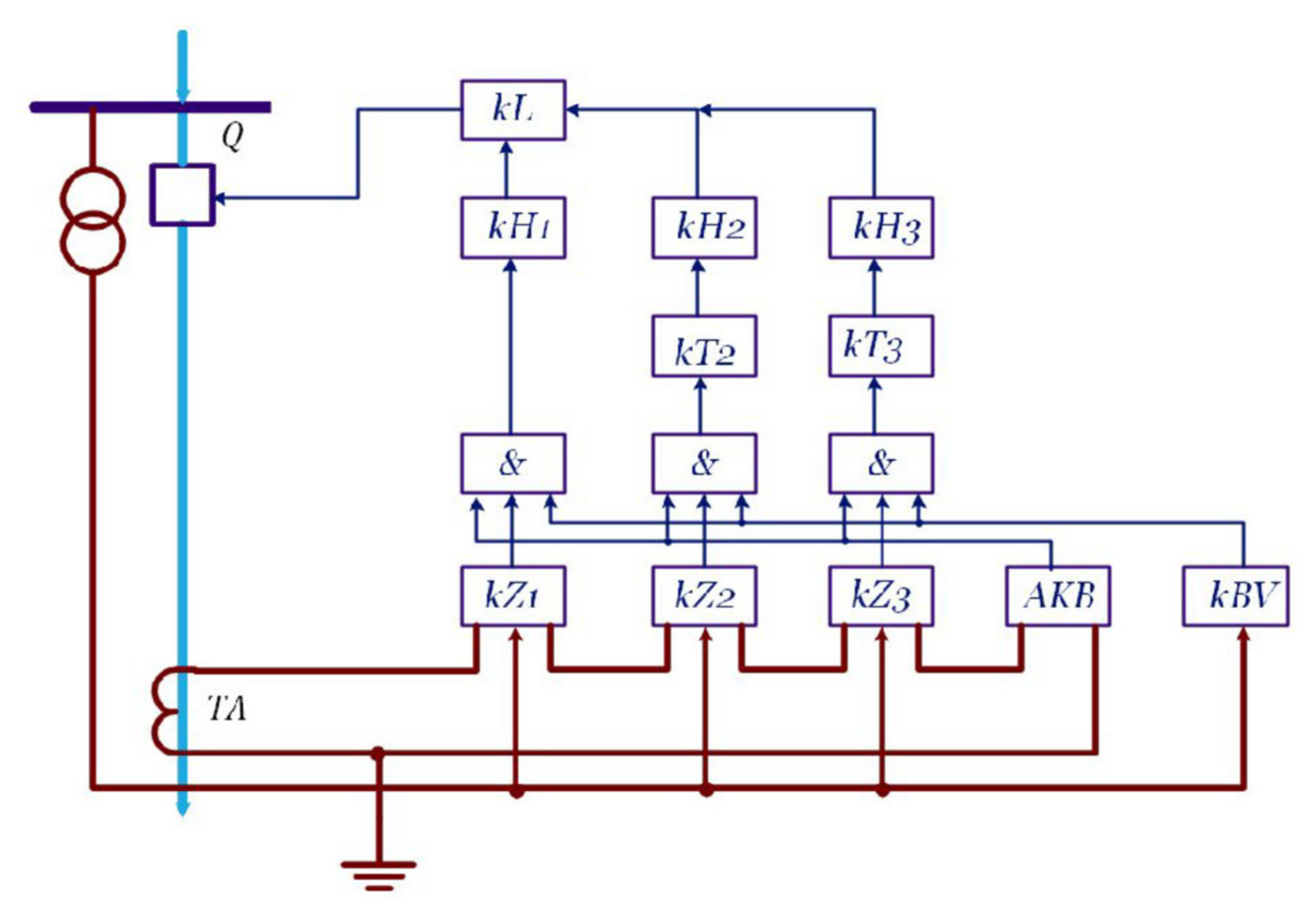
One of the typical options for performing three-stage distance protection is shown in Figure 1.

The single-phase short-circuits resistance at the input of the measuring device is greater than the multiphase short-circuits one at the same point, therefore the resistance measuring device cannot unnecessarily come into action [17]. The protection setpoint directly depends on the resistance, i.e., under certain conditions it is proportional to the distance between the protection and the short circuit. So, it is important to understand whether the protection will work correctly for this type of damage provided that variable external environmental parameters are neglected.

The active and reactive resistances of the overhead line are affected by external climatic factors that are not taken into account in the calculations. So, these variable factors affect the accuracy of damage detection. Line resistance z_l is calculated by the formula

$${\underset{¯}{z}}_l=\left({\underset{¯}{r}}_0+j{\underset{¯}{x}}_0\right)L_l,$$

(3)

where x₀ is the linear inductive reactance of the positive sequence, Ohm/km; r₀ is the linear active resistance of the positive sequence, Ohm/km; L₁ is the line length, km. The overhead power line is a distributed circuit. The assumptions about the concentration of actually distributed parameters are valid for overhead lines with length not exceeding 300–350 km [18].

Further analyze the influence of the finite conductivity of the ground and changes in environmental parameters on the longitudinal elements (resistances) and transversal elements, i.e., the conductivity of the U-shaped equivalent circuit (Figure 2). The equivalent circuit of the OHL consists of the longitudinal elements—impedance: Z= r + jx_L, and the transversal elements—conductivity: Y = g + jbC [19].

We analyze the impact of changes in atmospheric conditions on the linear parameters of an overhead power transmission line. As a rule, the linear parameters of the power transmission line are taken constant, standardized in the reference literature. These parameters are calculated for normal external factors (ambient temperature of 20 °C, sunny, soil resistance under the OHL is constant, etc.). However, in real OHL operating conditions, climatic conditions change significantly depending on the month and the climatic zones.

The relationship between the active resistance and the wire temperature is determined by the formula [20]:

$$R_{0t}=R_{020}\left(1+\alpha \left(t_{wire}-20\right)\right),$$

(4)

where R₀₂₀ is the reference specific resistance at a wire temperature of 20 °C; t_wire is the wire temperature, °C; α is the temperature coefficient of electrical resistance, Ohm/°C.

The OHL wire temperature depends on the ambient air temperature and current flowing through it. At the limiting current loads in terms of heating conditions, the wire temperature can reach +70 °C, and at low ambient temperatures and low loads it can be up to −50 °C. Therefore, the specific resistance can increase by 20% and decrease by 30%. The steady-state wire temperature is determined from the equilibrium condition for any operation mode of the overhead line [20]:

$$I^2{R}_{020}\left(1+\alpha \left(t_{wire}-{20}^{\circ }\right)\right)=\sigma F\left(t_{wire}-t_{amb}\right)$$

(5)

where I is the current along the wire, A; σ is the heat transfer coefficient equal to the amount of heat removed in 1 s from 1 cm² of the wire surface at a temperature difference between the wire and the environment of 1 °C, W/m²·°C; F is the wire cooling surface, cm²; $t_{amb}$ is the ambient temperature, °C.

The heat transfer coefficient can be defined as [21]:

$$\sigma ={\sigma }_l+{\sigma }_c=2.8\left(100+0.6\left(T_{wire}-273\right)\right)\cdot {10}^{-2}+8.95\sqrt{\frac{p\cdot \upsilon }{d}}$$

(6)

where σ_l is the heat transfer coefficient, determined by the transfer of heat by radiation, σ_c is the heat transfer coefficient, determined by convection, p is the air pressure, Pa; T_wire is the wire temperature, K; υ is the speed of air movement near the wire, m/s; d—wire diameter, m.

The wire temperature is affected not only by the wind speed, but also by current passing along the line and the ambient temperature. Taking into account expression (6), the temperature of the overhead line wire is found from Equation (5):

$$t_{wire}=\frac{I^2{R}_{020}+\sigma F{t}_{amb}-20\sigma F}{\sigma F-I^2{R}_{020}\alpha }+20.$$

(7)

According to the requirement of the Russian State Standard GOST 839-80 “Non-insulated wires for overhead power lines” the long-term permissible temperature of wires during operation should not exceed 90 °C, the flow of current through the wire leads to its heating. This means that it is possible to pass through the wire a current exceeding the maximum permissible (emergency maximum permissible current), which is 30% of I_per for a short period of time, while ensuring its mechanical resistance. This can be performed to make the experimental analysis of factors affecting the temperature of the wire more clear, while holding time of current relay protection is increased to eliminate operation with further disconnection of the test line. At low and medium currents (as compared with the permissible one I_per), flowing along the overhead line and not large wind loads, significant changes in the wire temperature occur mainly due to fluctuations in the ambient temperature. If the current load is more than 30% of the permissible line current and the wind speed is not high, then the current flowing along the conductor has a noticeable effect on its heating. With an increase in wind speed, heat dissipation significantly improves even with a large flowing current [21,22] (Figure 3).

Analysis of the operation temperature conditions of wires of various cross-sections used in overhead lines with a voltage of 110 kV and higher showed that the main relationships between wire temperature and the flowing current, ambient temperature, wind speed are similar to those shown in Figure 3 for the AC-120 wire. Consequently, the relationship between the resistance of the overhead power line wire and the ambient temperature for different brands of conductors will be the same as that shown in Figure 4.

Figure 3 and Figure 4 show that the temperature of the conductor does not go below −40 °C and above 70 °C, even for the conditions of low wind speed and line current equal to the permissible one. So, we analyze the relationship between the resistance of the overhead power line wire and temperature $R_{0t}=f\left(t\right)$ in the specified temperature range (Figure 5). For distribution networks the most common voltage is 110 kV, so for the analysis of overhead lines we use the AC steel-aluminum wire with a cross section of 120 mm² with linear parameters r₀ = 0.249 Ohm/km, x₀ = 0.427 Ohm/km, b₀ = 2.66 S/km.

The graph shows that an increase in wire temperature by 10 °C leads to an increase in wire resistance by 4%. Specific reactance depends on flux linkage, which in turn depends on the relative position of wires, taking into account the penetration of the magnetic flux into the ground surface.

Further we determine the reactance of the overhead power line taking into account the finite soil conductivity. If the ground is considered as a conductor with large dimensions, through which an alternating current flows, then due to the surface effect it will not be distributed evenly in the soil. The approximate analysis of the overhead power transmission line parameters considers the ground conductivity as an infinite value and it is assumed that the total current is concentrated on its surface. In fact, current penetrates to a certain depth, depending on the soil resistance. Taking into account that the soil is homogeneous, current decreases with distance from the wire inward and in both directions. A method for analyzing the influence of the finite conductivity of the ground was proposed by Rudenberg [23].

We get

$$\begin{array}{l}{\underset{¯}{Z}}_s=\frac{{\underset{¯}{E}}_s}{\underset{¯}{I}}=\left({\pi }^{2}f+j4\pi f\ln \frac{0.178}{h\sqrt{f\gamma \cdot {10}^{-9}}}\right)\cdot {10}^{-9}\\ =\left({\pi }^{2}f+29f\lg \frac{0.178}{h\sqrt{f\gamma \cdot {10}^{-9}}}\right)\cdot {10}^{-4}\end{array}$$

(8)

Decompose the impedance into active and reactive components, then

$$R_s={\pi }^{2}f\cdot {10}^{-4}$$

(9)

$$X_s=29f\lg \frac{0.178}{h\sqrt{f\gamma \cdot {10}^{-9}}}\cdot {10}^{-4}$$

(10)

With an increase in the frequency and conductivity of the soil, the magnetic flux, which is closed in the ground, will decrease, since the degree of inhomogeneity of the current distribution in the soil will increase. If the soil is taken as an infinitely conducting surface, then all the reverse current would be concentrated on the surface of the cylinder recess (ground) and there would be no need to consider the adhesion field.

To accurately determine the wire impedance, taking into account the ground conductivity, it is also necessary to take into account the active resistance of the wire itself and the adhesion of the wire to the part of the flow that is closed in air.

Determine the reactance created by a part of the flow that closes in the air, which in turn is created only by the wire current and coincides with it in phase, as for one wire of a one-phase two-wire line, provided that the distance between the wires D is numerically equal to the suspension height h of the considered wire [24].

$$X_{air}=29f\lg \frac{h}{r_{wire}}\cdot {10}^{-4}$$

(11)

And the inductance corresponding to the part of the flow closing in the air will be equal to:

$$L_{air}=4.6\lg \frac{h}{r_{wire}}\cdot {10}^{-4}$$

(12)

Taking into account expressions (9)–(11), the impedance of the wire is

$$\begin{array}{l}{\underset{¯}{Z}}_{wire}={\underset{¯}{R}}_{0t}+{\underset{¯}{R}}_{soil}+j{\underset{¯}{X}}_{soil}+j{\underset{¯}{X}}_{air}=\\ =\left[R_{020}\left(1+\alpha \left(t-{20}^{\circ }\right)\right)+\left({\pi }^{2}f+j29f\lg \frac{0.178}{r_0\sqrt{f\gamma \cdot {10}^{-9}}}\right)\cdot {10}^{-4}\right]\end{array}$$

(13)

According to expression (13), we divide the impedance of the wire into active and reactive components:

$${\underset{¯}{Z}}_{wire}={\underset{¯}{R}}_{wire}+j{\underset{¯}{X}}_L,$$

(14)

$$R_{wire}=\left(R_{020}\left(1+\alpha \left(t-{20}^{\circ }\right)\right)+{\pi }^{2}f\cdot {10}^{-4}\right),$$

(15)

$$X_L=29f\lg \frac{0.178}{r_{wire}\sqrt{f\gamma \cdot {10}^{-9}}}\cdot {10}^{-4}.$$

(16)

With an increase in the frequency and conductivity of the soil, the magnetic flux, which is closed in the ground, will decrease, since the degree of inhomogeneity of the current distribution in the ground will increase. Reactance is created by a part of the flow that closes in the air, which in turn is created only by the wire current and coincides with it in phase. To accurately determine the wire impedance, taking into account the ground conductivity, it is also necessary to take into account the active resistance of the wire itself and the wire adhesion to the part of the flow that is closed in air.

Expression (16) shows that the reactance does not depend on the height of the wire suspension, since an increase in the height of the suspension decreases the relationship between Xs and the flow that closes in the ground, but at the same time, X_air increases due to an increase in the flow that closes in the air. The wire reactance X_wire is usually determined by the method of image charges, i.e., the system “wire—imaginary wire passing underground” is considered. A distance between the wires D_s is chosen so that the wire resistance of the two-wire line is equal to the wire resistance of the “wire-ground” system.

$$D_s=\frac{0.178}{\sqrt{f\gamma \cdot {10}^{-9}}}\mathrm{cm},$$

(17)

where f is the frequency, Hz; γ is the soil conductivity, S.

Reactance of the conductor of the “wire-ground” system is

$$X_{wire}=29f\lg \frac{D_s}{r_0}\cdot {10}^{-4}\mathrm{Ohm}/\mathrm{km},$$

(18)

where r₀ is the wire radius, m.

From expressions (17) and (18), it follows that the wire reactance depends on the soil resistance, which varies over a wide range under the influence of temperature, humidity, etc. [25].

For a more accurate assessment of the soil resistance, we will consider it two-layer. The first layer is 2.5 m deep. The depth of the second layer is determined using the method of image charges, as half the double height of the suspension of the overhead power line wire above the ground’s surface. Then the equivalent resistance is

$${\rho }_{eqv}=\frac{h}{{\displaystyle \sum _{k=1}^3\frac{\Delta d_k}{{\mathsf{\rho }}_k}}+\frac{\Delta d_2}{{\mathsf{\rho }}_2}},$$

(19)

where h is the height from the imaginary wire located in the ground to the ground surface, m; ∆d_k is the maximum depth of soil soaking, m; ∆d₂ is the soil thickness not subject to seasonal changes in moisture content, m; ρ_k is the soil resistance in the section ∆ d_k, Ohm/m; ρ₂ is the soil resistance in the section ∆d₂, Ohm/m.

$$\Delta d_2=h-{\displaystyle \sum _{k=1}^3\Delta d_k}$$

Figure 6 presents the relationship between the wire reactance on seasonal fluctuations in moisture and temperature for various soil resistances.

Figure 6 shows that the trends of the curve changes by months coincide for various soil resistances. Therefore, regardless of the soil structure, a clear seasonal dependence remains, which must be taken into account when calculating the wire resistance χ.

Figure 7 presents the wire resistance taking into account the final conductivity of the ground, but without the seasonal coefficient. For this case the error was 7–8%.

When calculating the reactance using the method of image charges, the influence of the ground is not taken into account, since it is assumed that the soil is considered an infinitely conducting surface (mirror). Therefore, the magnetic field lines are closed only in air, and the return current is concentrated on the ground’s surface, and the distance between the imaginary wire and wire of the overhead power transmission line is taken to be equal to the double height of the suspension 2h (Figure 8).

In fact, the ground has a finite conductivity, therefore, when applying the method of mirror charges, this must be taken into account by placing a “mirror” at a distance of 0.5 Ds from the axis of the wire (Figure 9).

An increase in the distance Ds (value of the order of 1 km) in comparison with D (value of the order of 10 m) does not entail a proportional increase in the reactance, since as the distance from the wire axis increases, the length of the field lines increases and H decreases, therefore, an increase in the flow interlocking with a wire strongly, lags behind the increase in the distance between the wire axes.

Compare X for a distance between the wires D = 5 m with X_wire for Ds = 935 m, the AC—120 wire radius in both cases r_wire = 0.00429 m.

$$X=0.145\lg \frac{5}{0.00429}=0.47\mathrm{Ohm}/\mathrm{km}$$

Reactance of the wire-to-ground loop from (18)

$$X_{wire}=0.145\lg \frac{935}{0.00429}=0.773\mathrm{Ohm}/\mathrm{km}$$

Ratio of reactances is:

$$\frac{X_{wire}}{X}=\frac{0.773}{0.47}=1.65\mathrm{for}\frac{D_s}{D}=\frac{935}{5}=187\text{.}$$

(20)

Figure 10 illustrates the change in the reactance of the AC-120 wire at different soil resistances. Therefore, if the determination of the reactance of the overhead power line wire by the method of mirror charges does not take into account the final conductivity of the soil under the overhead line, then the calculation error will be about 65%. The reference value of the reactance does not take into account the conductivity of the soil, therefore, it differs from the calculated one, taking into account the final conductivity of the ground, almost twice.

Determine the impedance of the wire

$$Z_{0wire}=\sqrt{R_{wire}{}^2+{\left(X_L-X_C\right)}^2}$$

(21)

Based on expression (20), we construct the dependence of the change in the active resistance of the AC-240 wire on the ambient temperature, taking into account the final conductivity of the soil (Figure 11).

Figure 11 shows that with respect to the constant value of the line impedance, which is taken into account in the calculations, the impact of the ambient air temperature significantly changes it. If we estimate the error at two extreme points (at a temperature of 40 °C and −40 °C), then the error will be 8% and 23% respectively. Taking into account the final conductivity for the same ambient temperatures, the error will be 48% and 19%.

3. Development of Algorithms for Distance Protection and Fault Location with an Adaptive Setpoint

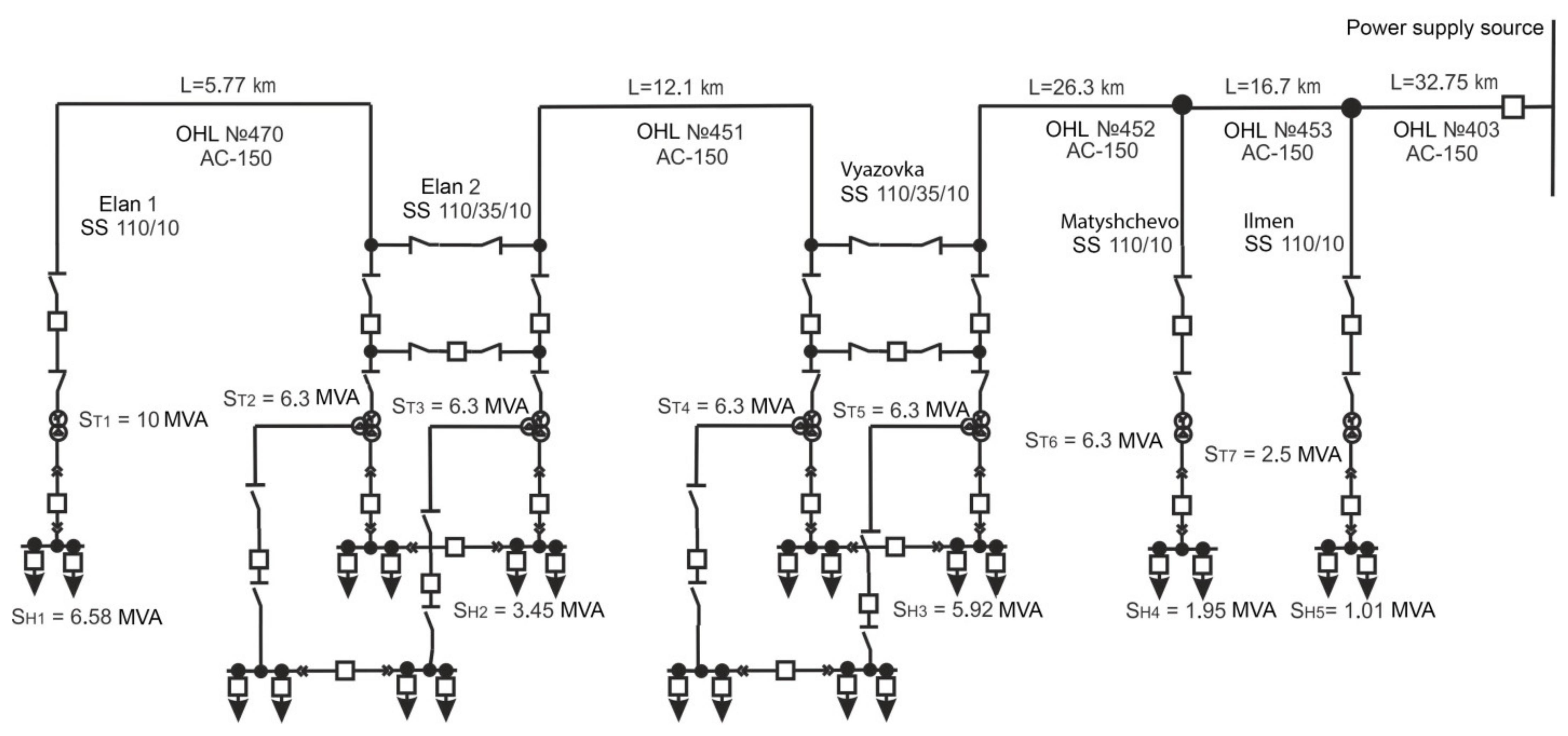
Further we calculate the short-circuit current for the overhead power transmission line of an electrical network (Figure 12). This overhead line is a main line with branch and double-ended substations, made of AC-150 single-circuit wire, its total length is 93.62 km.

The influence of external factors on the short-circuit current is plotted in Figure 13, the short-circuit currents for various types of damage were determined for the soil resistance of 20 Ohm·m.

The probability of short circuits in 110 kV electrical networks for various types of damage is distributed as follows: 4% of damage is caused by three-phase short-circuits, 8% by two-phase to ground, 5% by two-phase, 83% is caused by one-phase short-circuits. Determination of the relay protection setpoint current based on the maximum three-phase short circuit current can cause incorrect actions of the relay protection devices. Therefore, calculations using a three-phase short-circuit current have the following errors in determining the current setpoint: 22% for a two-phase short circuit, 9% for a one-phase short circuit, 7% for a two-phase to ground. The calculations were made with a resistance soil 20 Ohm·m (Figure 13).

Changes in soil resistance affect only types of damage, for which a zero-sequence current appears. So, one-phase and two-phase short circuits to ground are taken into consideration. When two factors (fluctuations in wire temperature and soil resistance) are taken into account, the calculation error for the operating current is up to 17% for a one-phase short circuit, and 7% for a two-phase to the ground.

The dynamics of change in protection resistance setpoints during a one-phase short circuit and change in soil resistance is shown in Figure 14. By analyzing the obtained data, it can be seen that the change in resistance is in the range from 14% (soil resistance ρ = 20 Ohm m) to 28% (soil resistance of ρ = 1000 Ohm m) relative to the resistance calculated for symmetric damage, therefore, distance protection, which is minimal, can do not work with asymmetric short circuits, provided that the soil dries out and increases its resistance.

The change in the resistance of the protection setpoints during a three-phase short circuit due to seasonal temperature fluctuations is not significant and can be completely neglected (Figure 15). Since the zero sequence is not included during calculations of this type of fault, the setpoint of distance protection does not change at different soil resistances, therefore, the calculation according to the traditional method gives such a significant error.

The resistance measuring element with the higher response setpoint is more sensitive. So, to reduce the “dead zone” length it is more expedient to use not tabular data as a setpoint, but that directly obtained from external parameters sensors. So, for an overhead line made of the AC-150 wire with a length of 93.62 km, the total reference resistance will be 43.47 Ohm. However, while taking into account soil resistance and ambient temperature it will be from 99 Ohm to 99.8 Ohm, therefore, the “dead zone” length will decrease by 2 times.

Figure 16 shows the change in current of a three-phase and two-phase short circuit as a function of the length of the overhead power transmission line. A straight line indicates the protection operation current, which is a constant value. The dead zone for a three-phase short circuit will be 31%, and 48.3%for a two-phase short circuit.

Consider changes in the “dead zone” length for various types of short-circuit currents and soil resistance under the overhead transmission line (Figure 16 and Figure 17).

Analysis of the plots shown in Figure 16 and Figure 17 shows that the “no operation” zone of the relay protection changes depending on the resistance of the ground under the overhead power line. The “dead zone” for a three-phase SC is 33.1%with a soil resistance of 20 Ohm·m, and 12.6% with a resistance of 1000 Ohm·m, the rest of the data are summarized in

Table 1. The “dead zone” length for various soil resistance.

No.	Type of Damage	“Dead Zone” Length,%
		ρ = 20 Ohm·m twire = 40 °C	ρ = 1000 Ohm·m twire = −40 °C
1	Three-phase short circuit	33.1	26.11
2	Two-phase short circuit	47.18	40.15
3	One-phase short circuit	26.11	19.08
4	Two-phase short circuit to ground	33.1	30.4

.

Calculating the relay protection setpoints without considering the seasonal change in soil resistance or its change along the power line can cause significant errors.

The scheme of intelligent system of distance relay protection with adaptive algorithms for determining the setpoints of the overhead power transmission line is shown in Figure 18. The head subsystem consists of a receiving modem and a dispatcher computer with installed software. The peripheral subsystem consists of measurement and transmission posts. The measurement posts are planned to be installed on the pores of overhead lines, the choice of location is based on the topography of the transmission line, in places most prone to ice formation and on heterogeneous ground reliefs, many years of experience in operating overhead lines are taken as a basis.

The measurement post consists of three galvanically unconnected parts with separate power supply: one of them (the wire temperature measurement module) is attached to the wire, the second is located on the support body, the third is in the soil near the support, directly under the overhead power line. It is proposed to implement this scheme using the commercially available elements and blocks, which speeds up the process of introducing the relay protection system into electrical networks.

The first part of the system uses the blocks of the ASTROSE automated system for detecting ice on the overhead line (OOO Sovtest ATE, Kursk, Russia). This system monitors ice, snow and wind loads on power lines, and controls the permissible current load of the wire. The modules are installed on wires mainly near the traverse of the supports within one span and are located at a distance of 500 m from each other.

To control humidity and ambient temperature, the DVT-02M microprocessor sensor (GK Teplopribor, Moscow, Russia) is used. It is used where corrosive substances can be present in the air, or short-term moisture condensation can occur. Moisture sensors are equipped with a new moisture sensing element with better temporal stability. Their parameter drift is not more than ±1.2% of relative humidity per year for a 50% relative humidity. A short-term operation of the humidity sensor at a temperature of +100 °C is acceptable.

The third part is a wireless digital conductivity sensor PASCO (Zeltix, Yekaterinburg, Russia). To determine the place of failure, the TDR-109 STRIZH-S power line reflectometer (Electronpribor LLC, Moscow, Russia) is used. TDR-109 STRIZH-S is a high-precision 3-channel digital reflectometer, specially designed to determine distances to any type of inhomogeneity and damage in power cable lines: open circuit, short circuit, coupling, cable splice, parallel branch, cable short circuit.

Ice detection on overhead transmission lines is also carried out using a reflectometer. The pulse signal during radar sounding of power transmission lines in the presence of ice deposits on it undergoes certain changes. This is explained by a change in the dielectric constant ε of the space between the wires of the line when ice appears. This increases the capacitance between the line wires. An increase in C entails a decrease in the wave resistance of the line. It also causes a decrease in the signal propagation speed along the line. In this case, an additional time lag of the pulse occurs due to a decrease in the propagation velocity of the signal and a decrease in the amplitude (attenuation) due to an increase in losses in the dielectric (ice deposits) due to its heating. Consequently, when ice appears, the pulses reflected from the above line inhomogeneities (considered as the reference points), will undergo an additional delay in arrival time and an additional decrease in amplitude. The combined manifestation of these factors is proposed to use as a criterion (indicator) of ice appearance on power lines.

Figure 19 presents the developed algorithm for the work of distance protection, which takes into account changes in external factors and adapts the response setpoint.

The calculation procedure for the proposed algorithm for determining the distance protection setpoints is as follows:

• Determine the parameters of power transformers of direct, reverse and zero sequence.
• Sensors of the ambient temperature, air humidity, wind speed and soil moisture under the overhead power line are installed on the protected overhead line. The measured parameters are transmitted via communication channels to the relay protection system for further analysis.
• Based on the data obtained, the actual longitudinal and transverse parameters of the overhead power transmission line of direct, reverse and zero sequences are calculated.
• Based on the OHL network data, the equivalent circuits are converted. The equivalent active, reactive resistances and equivalent EMF are determined.
• The impedance of the overhead power transmission line is calculated based on data on external environmental factors and the resistance unit settings are automatically set.
• In case of a short circuit on the protected line, we receive data on the line operation mode from current and voltage transformers.
• The fault resistance Z_c is compared with the protection setpoint Z_p, if Z_c < Z_p, the protection is activated.

When calculating the protection setpoint taking into account the external environmental parameters, it becomes possible to reduce the “dead zone” of the first stage of distance protection, due to the use of overhead line parameters that actually show the state of the line. The “dead zone” appears at the end of the protected line, because due to the long length of the fault resistance Z_c becomes less than the protection setting Z_p.

Distance protections have been used for a long time to protect networks of complex configuration and high voltage. The executive base of the resistance relay underwent changes from electromechanical to microprocessor, but the changes were more related to the hardware, and not the algorithms of operation. The main disadvantage of current protection is the dependence of the area of their action on the short-circuit current, which in some cases does not allow to achieve sufficient sensitivity of current protection, especially for its high-speed steps. In addition, in complex networks (for example, in a ring network with two power supplies), selectivity of current protection cannot be ensured. The use of the setpoint adaptation algorithm in distance protection allows one to take into account the decrease in the short-circuit current at the end of the protected line, to automatically set the resistance response setpoint, reflecting the real longitudinal and transverse parameters of the overhead line, thereby reducing the length of the “non-operation zone” and increasing the sensitivity of this type of protection.

To restore the normal operating mode of electric power systems, and to reduce damage and costs, it is necessary to quickly and accurately determine the fault locations. These requirements are satisfied by remote damage search methods, provided that the calculation accuracy is increased, Figure 20. As a rule, the calculation of OMP setpoints is based on the short-circuit currents, which directly depend on the longitudinal and transversal parameters of the protected power line.

To detect the fault, data on the external parameters of the environment are used, obtained from sensors installed on the overhead line. Reference values are not used, since it does not show the real picture of what is happening on the overhead line. As a result, the accuracy of fault detection on the overhead line is significantly increased.

Based on the developed algorithms, an intelligent system of the relay protection system is proposed. It forms a control action based on objective data received from sensors installed on the power transmission line in real time. This system has an increased protection sensitivity coefficient, allows one to reduce the “dead zone”, thereby increase the reliability of the installed protections. New algorithms for the operation of the relay protection device were developed, which reduce the number of “false alarms” and “failures”. A program that implements the developed algorithms was developed, which allows one to calculate the trigger parameters and determine the type and location of damage.

4. Conclusions

• The operating experience of relay protection systems shows that the level of setpoints is influenced by climatic factors and seasons. Therefore, to increase the reliability of the relay protection system, it is necessary to introduce an automatic current correction unit setpoints into the system.
• The relationship between the longitudinal and transversal parameters of power transmission line and the climatic factors of the environment was proved. Thus, at the current load of more than 30% of the permissible line current and not a high wind speed, the current passing through the conductor has a noticeable effect on its heating. At low and medium currents relative to the permissible, passing through the overhead line and not high wind loads, the change in the resistance of the wire occurs due to fluctuations in the air temperature.
• An increase in the wire temperature by 10 °C leads to an increase in the wire resistance by 4%, the error, relative to the constant active resistance, at the two extreme points is from 8% to 23%. When the final soil conductivity is taken into account the error reaches 19–48%.
• Relay protection and OMP devices must be installed on overhead lines with sensors of wire temperature and soil moisture, information from which at the time of the accident will be transmitted to the computing unit. The place of damage is calculated taking into account the correct data on the parameters of power line.
• An algorithm for intelligent remote relay protection was developed. It takes into account changes in external factors and adaptive calculation of the response resistance, which will reduce the length of the “dead zone” and increase the sensitivity of protection at the end of the line.