Abstract
Distributed energy resources (DERs), including renewable energy resources (RESs) and electric vehicles (EVs), have a significant impact on distribution systems because they can cause bi-directional power flow in the distribution lines. Thus, the voltage regulation and thermal limits of the distribution system to mitigate from the excessive power generation or consumption should be considered. The focus of this study is on a control strategy for DERs in low-voltage DC microgrids to minimize the operating costs and maintain the distribution voltage within the normal range based on intelligent scheduling of the charging and discharging of EVs, and to take advantage of RESs such as photovoltaic (PV) plants. By considering the time-of-use electricity rates, we also propose a 24-h sliding window to mitigate uncertainties in loads and PV plants in which the output is time-varied and the EV arrival cannot be predicted. After obtaining a request from the EV owner, the proposed optimal DER control method satisfies the state-of-charge level for their next journey. We applied the voltage sensitivity factor obtained from a load-flow analysis to effectively maintain voltage profiles for the overall DC distribution system. The performance of the proposed optimal DER control method was evaluated with case studies and by comparison with conventional methods.
1. Introduction
In recent decades, the concept of a DC microgrid has been proposed to improve the local reliability and flexibility of electric power systems comprising distributed energy resources (DERs), AC and/or DC loads, and energy-storage units [1,2,3]. DC microgrids combined with renewable energy sources (RESs) such as photovoltaic (PV) plants, energy-storage systems (ESSs), and electric vehicles (EVs) are the preferable solution for effectively integrating and improving the energy efficiency of electric loads using DC power converters [4].
Microgrid operators can profit from supplying reliable power for electric loads and also by selling surplus power generated by DERs to the grid. The profit can be increased by effectively controlling the power generation and consumption in the microgrid with various DERs and controllable loads. This can be achieved by establishing not only a sophisticated energy-management system with high data processing and communication speed, but also a reasonable and efficient energy-price policy for the microgrid. In addition, it is essential to link up with various incentive systems and ancillary service markets provided by electric power companies [5].
There have been various optimization approaches applied to microgrids; these include classic and artificial intelligence techniques, such as particle-swarm optimization (PSO) [6], genetic algorithms [7], or adaptive differential evolution algorithms [8]. In [7], the authors formulated an optimal power flow problem using a genetic algorithm to minimize the total operation cost of a DC microgrid while considering real-time pricing. The total operating cost covered the operation cost of utility grids, renewable energy resources, energy-storage systems, and fuel cells. Similarly, the authors in [8] suggested an adaptive differential evolution algorithm to minimize the operating cost of DC microgrids under real-time electricity prices. In [9], the authors suggested an optimal design and model predictive control (MPC) of a standalone hybrid renewable energy system (HRES). In the paper, the authors focused on a techno-economic analysis with an optimized sizing of a HRES components to meet the residential load demand of a specific area.
EVs will be an important component of the electric-power network in the near future. The widespread deployment of EVs might introduce a solution to the world’s fossil-fuel shortage, as well as the air-pollution crisis [10,11]. The goal of emissions reduction can be achieved by the proper and optimal utilization of EVs as energy-storage devices and loads in the power system integrated with RESs [12,13,14,15]. Beyond these advantages, connecting EVs to the power network could bring about many technical challenges that need to be addressed properly. The authors in [16] proposed to use an energy-storage system for EV charging and discharging stations to achieve better utilization of intermittent PV systems for EV charging. The approach in [16] can minimize the overall operating cost of the parking station by prioritizing the utilization of energy from RES, ESS, and the scheduling of every EV’s charging and discharging. This paper focuses on optimal-operation algorithms to minimize the operation cost of a DC microgrid with various DERs, such as RES and EVs.
Voltage regulation is another important issue in the low-voltage DC (LVDC) distribution system. Because of the low voltage level (1500 VDC), the voltage profiles in the overall LVDC distribution system are very sensitive to variations in the load and DER. Hence, changes in the load or PV-plant power generation could easily cause the voltage profiles in the DC distribution system to drop or rise out of the normal standard range, which is normally defined as 0.95 to 1.05 per-unit (p.u.) [17]. Many researchers have focused on voltage regulation in a DC distribution system. The authors in [18,19] proposed a voltage-control algorithm by coordinating the main AC/DC converter and DER scattering in a distribution system. They calculated voltage sensitivity factors (VSFs) based on the solution of load-flow analysis to calculate the relevant power injection or absorption to compensate for the voltage problems. In their approach, the power compensation for voltage control was computed based on the rank of the sensitivity factor, and the DER with the highest sensitivity value could be considered as the highest priority for voltage regulation. However, these control approaches did not consider the generation cost of the DERs or the total operating cost. Furthermore, the authors applied the voltage-control algorithm only after the voltage problem occurred, as it is difficult to control the voltage before this. In addition, their method did not consider the price of voltage compensation.
In this paper, we propose a control method for DERs such as RESs and EVs that can be implemented in the energy-management system (EMS) for a DC microgrid. The vehicle-to-grid (V2G) capability is also exploited in this research. With V2G capability, the state-of-charge (SoC) of an EV battery can go up or down depending on the electricity price, voltage profiles, and grid demand. Hence, we propose an optimal control strategy for the distributed energy resource in a DC microgrid that takes energy-cost reduction and voltage regulation into account.
The main advantages of the proposed optimization scheme are as follows. First, we apply an advanced forecasting algorithm into load consumption and solar irradiation for PV generation based on a recurrent neural network (RNN) [20] to predict the load and PV outputs every hour for the next 24 h. Second, we use the 24-h rolling-horizon window with 1-h sliding steps so that we can optimally operate DERs by considering the next 24-h microgrid operation. The sliding-window concept can deal with the uncertainty issue of EV connections to the microgrid by updating the new EV connections every hour. The time-varying electricity price with time-of-use (ToU) can be applied to the 24-h cost-optimization process. Third, we calculate the VSFs based on the Jacobian matrix of the system and load-flow analysis. Therefore, we can calculate the required amount of power injection/curtailment for the DERs by considering line losses and voltage drops in the distribution lines. This method can be applied to both radial and mesh networks. Moreover, we propose constraints for voltage regulation based on the sensitivity factor and voltage deviations.
This paper is organized as follows. Section 2 contains an introduction of the EMS for a DC microgrid. In Section 3, we formulate an objective function for DER control. Section 4 comprises an explanation of the optimal DER control scheme. Last, in Section 5, we report the experimental results of various simulation studies to verify the effectiveness of the proposed optimal strategy method compared to conventional methods [18,19].
2. The EMS for a DC Microgrid
2.1. Configuration of the DC Microgrid
Consider a DC microgrid system consisting of the main AC/DC converter and other entities such as a number of EV charging stations, PV power generation, and AC and DC loads. An AC/DC converter interconnects the DC microgrid to a 22.9 kV medium voltage AC grid, whereas other entities connect to the system via power electronic devices. As shown in Figure 1, the EMS for the DC microgrid receives the electricity tariffs for the ToU for load consumption and electric vehicle charging from the utility distribution company (distribution system operators/distribution network operators (DSO/DNO)). The EMS for the DC microgrid (MG-EMS) communicates with the other entities in the DC microgrid via an ethernet connection, which allows the MG-EMS to monitor and control the charging and discharging actions of a connected EV battery, as well as the PV power generation and/or the load shedding.
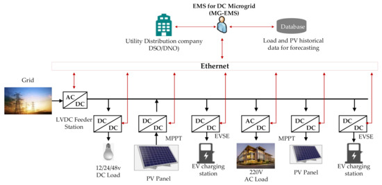
Figure 1.
A typical LVDC distribution system and control-base architecture for the voltage-control algorithm.
2.2. The Objective of DER Control in a DC Microgrid
The aim of using an EMS for a DC microgrid in the LVDC distribution system is to meet the following fundamental objectives:
- The MG-EMS was designed to minimize the total operating cost of the microgrid in terms of the load consumption and the EV charging cost. The MG-EMS tries to charge the EV during a high PV generation period or a low electricity tariff period. During peak-loading conditions, the MG-EMS encourages the EVs to discharge their battery to enable shifting of the peak load.
- The EMS for the DC microgrid controls the DERs to maintain the voltage profiles on the distribution lines within the normal range. Because of the low voltage level, the voltage profiles in the DC distribution system are very sensitive to variations in the load consumption and DER generation. Small changes in the loads and PV plants can easily make the voltage profiles on the distribution system drop or rise out of the normal range, which is defined as within ±5% of the rated voltage. Therefore, voltage control is one of the most interesting issues in DC microgrid operations.
- The MG-EMS can curtail DERs such as PV plants for overvoltage regulation in some critical cases.
To obtain the above objectives, the following control variables are considered:
- Two continuous variables representing the EV charging and discharging rates of the connected EV. Based on these, the MG-EMS can assign EV charging or discharging to minimize the operating cost of the DC microgrid and maintain the voltage profiles in the distribution lines.
- PV output-power curtailment. The EMS for the DC microgrid can curtail the PV power via the power electronic controller to reduce the overvoltage problem when the plugged-in EV batteries cannot solve it.
- Load shedding/shifting. The MG-EMS can shift or shed loads if the discharging of connected EV batteries cannot solve the undervoltage problem.
3. Formulation of Objective Function for DER Control
3.1. Statement of the Problem
In this study, the operational cost of a DC microgrid is minimized based on information concerning the loads, connected EVs, and PV generation. However, the loads and PV output power are known to be time-varying uncertainty factors. PV output power depends on the availability of solar irradiation related to the weather conditions, whereas load consumption depends on the consumer’s behavior. To solve the uncertainty problem, we apply an advanced forecasting algorithm for the load and PV plants based on an RNN [20] to predict the load and PV requirements 24 h ahead.
The ToU rates for EV charging and load consumption vary over time. They are not fixed for predetermined time intervals, but vary depending on the load period categorized as off-peak, mid-peak, and on-peak. Thus, we apply the 24-h window with 1-h step sliding on the horizon to encourage the charging of connected EVs during the off-peak period to minimize the EV charging cost and discharging during the on-peak period. This shifts the load, thereby minimizing the cost of the load consumption. The details of the sliding window are described in the next section.
Voltage magnitude is one of the most important parameters for LVDC distribution systems. However, the voltage profiles in the LVDC distribution system are very sensitive to variations in loads and PV plants because of the low voltage level. Hence, changes in the load, PV power generation, and EV charging/discharging power can easily cause the voltage profiles in the distribution system to be outside of their normal ranges. Hence, we suggest the VSF for optimizing the operational cost of the microgrid without affecting the voltage profiles. Moreover, inequality constraints between the total voltage compensation from EV discharging power and the maximum voltage deviation are proposed to ensure the stability of voltage profiles during the optimization horizon.
Finally, the SoC of the EV batteries requests the conditions required to avoid overcharging and deep discharging to determine the SoC level at the time of leaving the charging station. To solve this problem, we use the SoC equations in every time interval and put them in inequality constraints for both the upper and lower limits and constraints for the departure SoC.
3.2. Definition of Objective Function
The total cost of load consumption can be reduced by increasing the PV power generation and discharging power from the EV. The objective function for the optimization is defined as follows:
where is the electric vehicle charging tariff; is the load consumption tariff at the j-th interval; the two continuous variables and are the EV charging and discharging rates of the m-th connected EV, respectively; and are the maximum charging and discharging power values provided to the m-th connected EV at the charging station, respectively; and are the total load consumption and PV power generation in the microgrid at the j-th interval, respectively; and signifies the connection state of the m-th EV at each time step. For the latter, we suggest using a binary parameter defined as:
where and are the plugged-in and disconnected times for the m-th EV. In particular, Equation (2) implies that is 1 when the m-th EV is plugged in, and , otherwise.
The EV charging and discharging power are respectively calculated from the charging and discharging rates as:
3.3. Equality and Inequality Constraints for Optimization
3.3.1. Voltage Regulation Constraints
We respectively define , the maximum voltage deviation of the k-th bus that has the lowest bus voltage at interval j, and , the maximum voltage deviation of the h-th bus that has the highest bus voltage at interval j, as:
where
To maintain the voltage profiles on the overall distribution system, we must always keep the maximum bus voltage less than the upper limit (1.05 p.u.) and the minimum bus voltage higher than the lower limit (0.95 p.u.), which is conducive to normal operation mode. To present this problem, we suggest the VSF defined as the effect of power variation control of the DERs at the i-th bus on the voltage compensation of the k-th specific bus. Based on the VSF, the total voltage compensation for the undervoltage problem from total EV discharging must be higher than or equal to the voltage deviation at the k-th bus, while the total voltage reduction for the overvoltage problem from overall EV charging must be higher or equal to the voltage deviation at the h-th bus, which can be respectively defined as follows:
where denotes the power injection from the m-th EV discharging action located at the i-th bus to compensate for the voltage at the k-th target bus at the j-th time step; represents the power absorption from the m-th EV charging action located at the i-th bus to reduce the voltage at the h-th target bus at the j-th time step; is the VSF defined as the effect of the power-variation control of the DERs at the i-th bus on the voltage compensation of the k-th specific bus at time step j.
The authors in [18,19] suggested that the VSF can be obtained from the Jacobian matrix of the LVDC distribution system as follows:
The Jacobian matrix corresponding to derivations of the active power from the bus voltage magnitude is obtained as follows:
- Off-diagonal elements:
- Diagonal elements:where N is the number of buses; and are the bus voltages at the k-th and i-th nodes, respectively; and G denotes the conductance matrix. The conductance matrix is similar to the bus admittance matrix for an AC distribution system, with the only difference being the absence of the reactance components.
According to Equations (10)–(12), the VSF can be calculated based on the conductance matrix and bus voltages, which can be easily calculated by solving the power-load-flow equations using the predicted load and solar irradiation.
3.3.2. EV Charging/Discharging Restriction Constraints
EV charging and discharging should be restricted depending on the voltage profiles in the overall distribution system. During each time interval, we check for any voltage deviations in the buses to define the operation mode. Based on the voltage deviations calculated using Equations (5) and (6), operations are divided into three modes:
- Normal operation mode ( and ). When there are no voltage problems, the EVs can be in idle mode or charging/discharging mode to minimize the total operational cost of the DC microgrid. To avoid violating the constrained maximum charging and discharging power and preventing the simultaneous charging and discharging of the connected EVs during the scheduling process, the following constraints are implemented:where is a binary variable that represents the charging and discharging status of the connected EVs at the time step j defined as:
- Undervoltage operation mode (). The EVs are restricted to either idle mode or discharging mode to avoid the worst undervoltage problems. The following constraints are implemented:
- Overvoltage operation mode (). The EVs are restricted to either idle mode or charging mode to avoid the worst overvoltage problems. The following constraints are implemented:
3.3.3. SoC of the EV’s Batteries
At step j, the SoC of each connected EV should be restricted by an upper SoC limit and lower SoC limit to avoid the overcharging and deep discharging of the battery, respectively. The SoC at each time step can be obtained by considering the initial SoC and incrementing or decrementing it due to charging or discharging of the EV battery, respectively. The SoC of the m-th connected EV at time step j, denoted as , is given by:
where represents the initial SoC of the connected EV m. Hence:
Each EV needs to be sufficiently charged to guarantee the minimum energy requirements for its next journey. For this reason, the SoC of the m-th connected EV must satisfy the departure limit when it leaves the charging station:
4. Optimal DER Control Scheme
4.1. Optimization with a 24-H Sliding Window
In each instant k, we optimize the total operation within 24 h based on the ToU rates, EV connection, and predicted load and PV power. However, the number of EVs joining the system is one of the unpredictable components, so it is difficult to optimize the EV charging and discharging cost in the time horizon. To solve this problem, the rolling horizon concept with 1-h sliding steps over 24 h is considered for reducing the effect of the uncertainty’s variables, such as EV participation and forecasting values of loads and PV [21,22,23]. The rolling-horizon strategy is described in detail in Section 4.2.
Figure 2 shows the updating scheme of the electric-vehicle participations using the rolling-horizon concept. In the first interval, the MG-EMS for the DC microgrid recognizes two EVs connected to the charging station, and the optimization process is executed based on the information on EVs 1 and 2, the forecasting values of loads and PV in the prediction horizon of 24 h. However, when another EV is connected in the second interval, the EMS detects EV 3’s connection and updates the SoCs of the three EVs. The EMS will re-optimize the system operation using the updated information on three EVs. Assuming that the EMS should obtain the initial SoC and the plugged-in and disconnected times for the EVs via the EV supply equipment (EVSE).
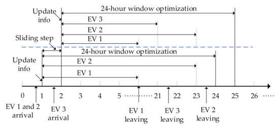
Figure 2.
The 24-h window optimization with 1-h sliding steps on the horizon.
4.2. The Proposed Procedure for the Optimal DER Control Scheme
The flowchart in Figure 3 shows the overall optimization process for minimizing the operational cost of DC microgrid. As shown in the figure, the proposed procedure is divided into four steps using the rolling-horizon concept: (i) forecasting the load and PV output power for the next 24 h, (ii) updating the current EV states, (iii) running optimization in the 24-h horizon, and (iv) deciding the optimal output. The outputs for the optimal process are the power scheduling for charging and discharging of the connected EVs.
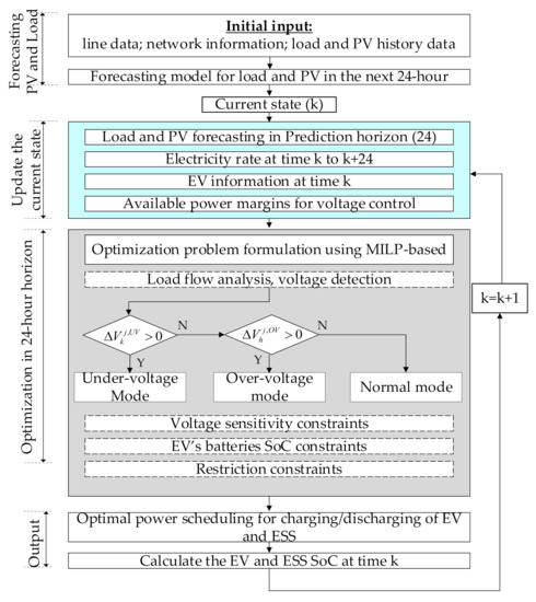
Figure 3.
Flowchart of the optimal scheduling scheme when considering voltage regulation.
- Step 1: The MG-EMS for the DC microgrid use the historic data of the load and PV plants as well as power-distribution network data such as line parameters and topology. A long short-term memory-based RNN (LSTM-RNN) process is used as the forecasting model for load and PV plant data for the next 24 h [20].
- Step 2: In the k-th time instance, the MG-EMS updates the information of the microgrid operation with time-varied electricity rates for EV charging and load consumption; EV data, including the current SoC level and the requested SoC for departure; the 24-h forecasting values for the load and PV power using the updated data; and the trained model in Step 1.
- Step 3: Based on the updated information in Step 2, we formulate the optimization problem using mixed-integer linear programming (MILP) to minimize the objective function defined in Equation (1) to reduce EV charging and electricity costs for the load consumption within 24 h. The SoCs of the EV batteries are calculated using Equation (20). The power flow is calculated in each interval time using the predicted load and PV power to determine the voltage profiles in the overall distribution system. The constraints for voltage regulation and EV charging/discharging operations from Equations (8) to (9) and (13) to (19), respectively, are added into the optimization process based on the operation modes to restrict the EV charging and discharging under the aforementioned voltage problems. Depending on which, the operation modes are divided into three principal modes (Figure 4):
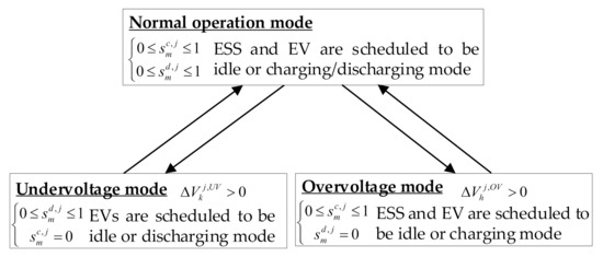 Figure 4. Operation modes for the scheduling scheme.
- ✓
- Normal operation. When there are no voltage problems, the EVs are in the idle or charging or discharging modes based on the electricity rate to minimize the operational cost of the microgrid.
- ✓
- Undervoltage mode. When there is an undervoltage problem at the time step, the MG-EMS schedules the EV to discharge to compensate. Load shedding is applied when EV discharging cannot solve the problem.
- ✓
- Overvoltage mode. When an overvoltage problem occurs due to overgeneration by the PV plant, the EVs are encouraged to charge as much as possible. Then, PV curtailment is used to reduce the overvoltage problem when EV charging cannot solve the problem.
- Step 4: The control signal for EV charging/discharging to the system is executed, then the SoC and the set of sampling instances are measured, after which Step 2 is repeated.
In general, EVs should be scheduled for charging during the off-peak period of the EV charging tariff in normal operation mode or during an overvoltage problem; discharging of EVs is encouraged in the on-peak period of the load consumption tariff or when an undervoltage problem occurs.
5. Case Studies
5.1. The LVDC Microgrid Model
To verify the performance of the proposed scheduling algorithm, we implemented a simulation model of an LVDC distribution system as shown in Figure 5, represented as a bipolar DC distribution system with positive and negative poles. The simulation model was a typical radial network with nine buses in which the rated voltage between two poles is 1500 VDC. The distribution lines were modeled as a 60 mm2 overhead cable with a line resistance of 0.313 Ω/km. The distances between buses are available in the figure. The loads and DERs were connected to two poles via power electronic converters.
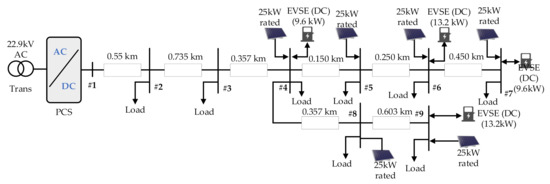
Figure 5.
Configuration of the LVDC distribution system for the simulation studies.
The window horizon for optimization was set as 24 h with a 1-h sampling interval. The electricity prices (ToU-based) used in this simulation were obtained from the Korean Electric Power Company (KEPCO), as shown in the next section. PV panels with a rated power of 25 kW were installed at buses #4 to #9.
EVSEs with V2G capability were installed at buses #4, #6, #7, and #9 and the charging/discharging capacity of the EVSEs were limited to 9.6, 13.2, 9.6, and 13.2 kW, respectively. We assumed various EV models with different battery sizes such as 25, 32, 35, and 42 kWh, respectively. Random arrival and departure of EVs were considered for realistic case studies. The initial and departure SoCs for each EV are reported in Table 1. The departure time for each EV was recorded by the MG-EMS, as shown in Figure 6 and Table 1. Moreover, the SOCs of the EVs were constrained by the upper and lower limits of 90% and 20%, respectively. The simulations were run using MATLAB 2019a, and the proposed optimization problem was solved using the CPLEX optimizer toolbox.

Table 1.
Initial information for the EVs in the simulation cases.
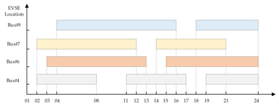
Figure 6.
Random EV arrival and departure information.
5.2. ToU-Based Electricity Rates
KEPCO has many different electricity prices depending on the tariff: residential, general, education, industrial, agricultural, street lighting, midnight power, and EV charging. In this study, we used the EV charging tariff as listed in Table 2 and Table 3.
Table 2.
The EV charging tariffs.
Table 3.
Season and time-period classification.
5.3. Simulation Results
Two case studies were considered to evaluate the performance of the proposed optimal control strategy. In Case 1, the system operation ran in normal mode with normal loading conditions over all of the optimization horizon. In Case 2, heavy loading was applied, in which the distribution system suffered an undervoltage problem in several time steps. In both cases, the results were compared to the conventional methods in [18,19], in which EVs were charged immediately after connecting to the system and discharging of the EV batteries was carried out to compensate for undervoltage problem based on the rank of the VSF. The conventional method did not consider the time-varying electricity price and cost reduction by shifting the EV charging and discharging time.
5.3.1. Case 1: Normal Operation
In this case, normal loading conditions were applied to the distribution system, and the MG-EMS ran the optimization process in every interval to find the optimal charging and discharging of EV batteries to minimize the operating and EV charging costs.
The 24-h power profiles of the PV at buses 4, 5, 6, 7 and the loads at buses 2 to 9 are plotted in Figure 7. Figure 8 shows the total net load in 24 h and the voltage profile with the lowest bus for Case 1. The total net load is defined as the difference between the total load consumption from buses 2 to 9 and total PV power generation from buses 4 to 9. The solid line with square dots in Figure 8 show that the peak loads were concentrated from 6:00 AM to 9:00 AM and 17:00 PM to 21:00 PM during the day. The solid line with circle dots in Figure 8 and the second column in Table 4 show the lowest voltages at the target bus, which were between 0.95 p.u. and 1.05 p.u. under normal loading conditions.
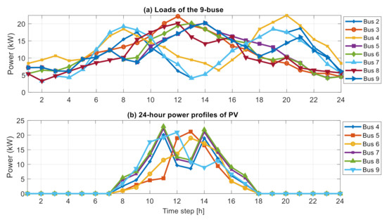
Figure 7.
Active power profiles of PV (generation) and load (consumption) for Case 1.
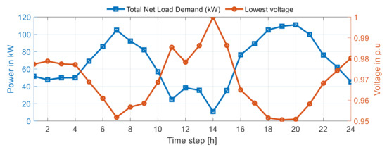
Figure 8.
The minimum voltage profiles in the distribution line according to loading condition for Case 1.
Table 4.
Voltage profiles and EV charging/discharging power for Case 1.
When the EVs described in Table 1 were connected to the system, the EMS for the DC microgrid ran the optimization process to optimize the total operating cost while maintaining the voltage profile in the normal range. The 4th to 7th columns in Table 4 report the results for EV charging and discharging to optimize the total operating cost. There were two EVs connected to EVSE 2 located at bus #6 within 24 h. The EVs were scheduled to charge during the low-price electricity period and discharge during the high-price electricity period to reduce the operating cost. For example, the EV plugged in at 3:00 AM and disconnected at 13:00 PM at the EVSE 2 was charged with 13.2 and 11.30 kW at 04:00 AM and 05:00 AM, respectively, when the electricity price was 57.60 KRW/kWh, and discharged 13.20 kW at 10:00 AM when the electricity price was 232.50 KRW/kWh. The charging and discharging processes always followed the voltage constraints to keep the voltage profile above the lower limit of 0.95 p.u. The third column in Table 4 lists the results of the minimum voltage in the distribution line. We can see that the lowest voltages were always higher than or equal to 0.95 p.u.
The 8th to 12th columns in Table 4 report the results for the voltage profiles and EV charging power using the conventional method. The EVs were scheduled to charge immediately after connecting to the system and to discharge when an undervoltage problem occurred. In this case, there were no voltage problems during the day, and so the EVs were charged immediately after being plugged into the system to reach the departure SoCs required by the EV owners.
Figure 9 shows the charging and discharging power of each EVSE compared to TOU EV charging price. It can be noted that the EV charging usually occurred during a low EV charging price in the proposed method. Figure 10 represents the minimum voltage of the distribution line for 24 h. Because of voltage control scheme, the lowest voltage could be maintained at more than 0.95 p.u.
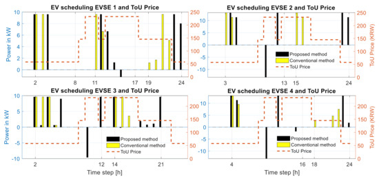
Figure 9.
EV charging/discharging power optimization for Case 1.
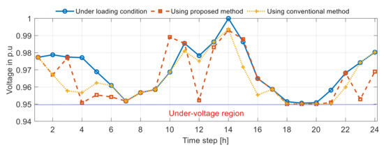
Figure 10.
Voltage profiles at the lowest bus voltage for Case 1.
Figure 11 shows the results of the SoC of the EV battery. The dashed blue lines in the figure show the results of the SoC of the EV of the proposed optimal strategy control, and the solid red lines represent the results of the conventional methods. The departure SoC of each EV reached the request from the EV owner as listed in the 7th column in Table 1.
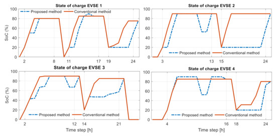
Figure 11.
SoC of the EV batteries at each EVSE for Case 1.
Figure 12 exhibits a comparison of the total operating cost, including the total load consumption cost and EV charging cost, between the proposed optimization method and the conventional method in a month. The figure shows that by using the proposed optimization approach, the DC microgrid operator could save KRW 360,225 per month, which is roughly about USD 327.50 per month.
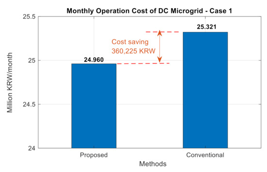
Figure 12.
Operating cost comparison between the proposed optimization and conventional methods for Case 1.
5.3.2. Case 2: Undervoltage Problem
In Case 2, high loading conditions were considered to evaluate undervoltage problems. We assumed that the total loads increased by 20% at time intervals 7:00 AM and 8:00 AM, and by 10% at intervals 18:00 PM and 19:00 PM compared to Case 1. Increasing the total loads caused an undervoltage problem at target bus 7 with values of 0.9436, 0.9481, 0.9473, and 0.9464 p.u. at intervals 7:00, 8:00, 18:00, and 19:00, respectively. The data of loads and PVs of the 9-bus DC microgrid are shown in Figure 13 with 24-h in time-varying format. Total loads and voltage profiles at the target bus are presented in Figure 14. The initial information on the EVs was similar to Case 1.
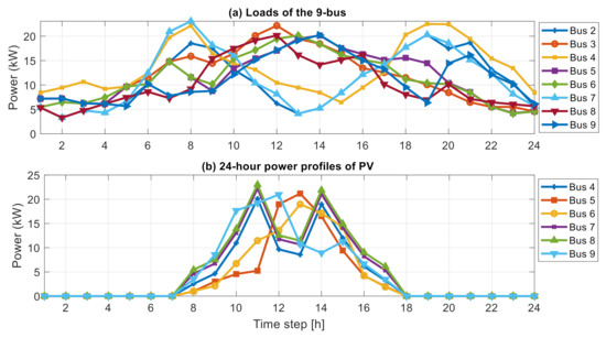
Figure 13.
Active power profiles of PV (generation) and load (consumption) for Case 2.
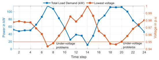
Figure 14.
The minimum voltage profiles in the distribution line according to loading condition for Case 2.
In each time step, the MG-EMS for the DC microgrid updated the EV arrival, initial SoC, and request for departure SoC, and predicted the load and solar power. The EMS ran the power-flow analysis to detect voltage violations. Then, the optimization process was executed to achieve the total cost optimization, voltage regulation, and EV departure SoC. Table 5 lists the results for EV charging/discharging power and voltage regulation in Case 2. The third column in the table shows that the undervoltage problems during intervals 7:00–8:00 AM and 18:00–19:00 PM were compensated for by EV discharging activity. The results of EV charging and discharging power are also compared to the conventional method in the table.
Table 5.
Voltage profiles and EV charging/discharging power for Case 2.
Figure 15 shows the results of the charging and discharging power calculations for EVs at four charging stations. Between 7:00 and 8:00 AM, the EVs at EVSE 1 and 3 were discharged to compensate for voltage problems. The EVs were also discharged during intervals when the electricity price was high, such as at 11:00 AM, and charged when it was low, such as at 12:00 PM. Figure 16 exhibits the voltage profiles at the target bus listed in columns 2, 3, and 9 in Table 5. It can be seen that the lowest voltage values were improved by both methods.
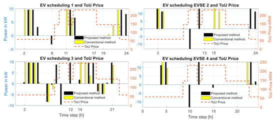
Figure 15.
EV charging/discharging power optimization for Case 2.
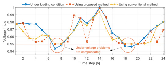
Figure 16.
Voltage profiles at the lowest bus voltage for Case 2.
Figure 17 shows the SoCs of the EVs, all of which were fully charged when reaching the requested departure SoC; these are listed in the last column in Table 1. Because the proposed method used a 24-h window, it can charge an EV more than the EV owner’s request and discharge the surplus energy during a high electricity price period. In this way, the proposed method can provide more economic solutions to DC microgrid.
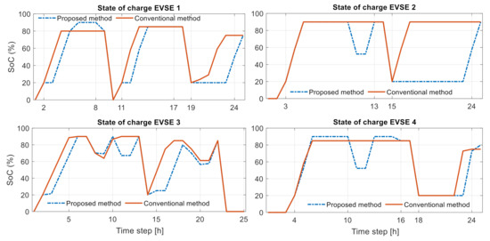
Figure 17.
SoC of the EV batteries at each EVSE for Case 2.
Figure 18 presents a comparison of the total operating cost using the proposed scheduling optimization and conventional methods for Case 2. We can easily see that the total cost savings by using our proposed algorithms is KRW 264,660 per month (about USD 240.60 per month) compared to the conventional method.
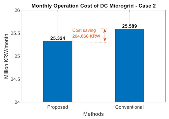
Figure 18.
Operating-cost comparison between the proposed optimization and conventional methods for Case 2.
6. Conclusions
In this study, we leveraged EVs available in a DC distribution system to optimize the total operating cost and control the voltage regulation. The proposed optimal control strategy was formulated using MILP in the 24-h horizontal with 1-h sliding steps. By using this, information such as load and PV power forecasting, ToU-based time-varying electricity price, EV arrival and departure time, and initial and departure SoC of EVs can be updated at each time interval to implement the optimization process. We applied an advanced forecasting algorithm based on an RNN to predict the load demand and the output of PV plants.
In this approach, we applied the voltage sensitivity factor concept, which is calculated from the power-flow analysis to ensure the voltage control in the proposed optimization. The VSF is to define the voltage sensitivity against power injection. Hence, it determines the effect of varying the power of the DERs at one bus on the voltage compensation at the other buses. In the optimization process, we considered the constraints of voltage regulation using VSF and voltage deviation; these constraints are to guarantee the overall voltage profiles will be within the normal range.
In normal operation mode, the proposed method encouraged EV charging at the low electricity price and discharging at the high electricity price to minimize the overall operating cost. On the other hand, when an undervoltage problem occurred, the EVs were prohibited from charging and encouraged to discharge to compensate for the voltage problem. Moreover, the constraints of the connected EVs were considered to satisfy the departure SoC level requested by the EV owner. The proposed method was compared with a conventional method in two case studies. The simulation results numerically verified that the proposed method is cheaper to run than the conventional method.
Author Contributions
Conceptualization, P.-H.T. and I.-Y.C.; methodology, P.-H.T.; investigation, I.-Y.C.; resources, P.-H.T.; writing—original draft preparation, P.-H.T.; writing—review and editing, I.-Y.C.; supervision, I.-Y.C. All authors have read and agreed to the published version of the manuscript.
Funding
This research was supported by the National Research Foundation of Korea (NRF) grant funded by the Korea government (MSIT) (No. 2019R1A2C1003880) and the Ministry of Science and ICT, Korea, under the ITRC (Information Technology Research Center) support program (IITP-2020-2018-0-01396) supervised by the IITP (Institute for Information and Communications Technology Promotion).
Institutional Review Board Statement
Not applicable.
Informed Consent Statement
Not applicable.
Data Availability Statement
Not applicable.
Conflicts of Interest
The authors declare no conflict of interest.
References
- Lonkar, M.; Ponnaluri, S. An Overview of DC Microgrid Operation and Control. In Proceedings of the IREC2015 the Sixth International Renewable Energy Congress, Sousse, Tunisia, 24–26 March 2015; IEEE: Piscataway, NJ, USA, 2015; pp. 1–6. [Google Scholar] [CrossRef]
- Magdefrau, D.; Taufik, T.; Poshtan, M.; Muscarella, M. Analysis and Review of DC Microgrid Implementations. In Proceedings of the 2016 International Seminar on Application for Technology of Information and Communication (ISemantic), Semarang, Indonesia, 5–6 August 2016; IEEE: Piscataway, NJ, USA, 2016; pp. 241–246. [Google Scholar] [CrossRef]
- Kumar, D.; Zare, F.; Ghosh, A. DC Microgrid Technology: System Architectures, AC Grid Interfaces, Grounding Schemes, Power Quality, Communication Networks, Applications, and Standardizations Aspects. IEEE Access 2017, 5, 12230–12256. [Google Scholar] [CrossRef]
- Sofla, M.A.; Gharehpetian, G.B. Dynamic Performance Enhancement of Microgrids by Advanced Sliding Mode Controller. Int. J. Electr. Power Energy Syst. 2011, 33, 1–7. [Google Scholar] [CrossRef]
- Shi, L.; Luo, Y.; Tu, G. Bidding Strategy of Microgrid with Consideration of Uncertainty for Participating in Power Market. Int. J. Electr. Power Energy Syst. 2014, 59, 1–13. [Google Scholar] [CrossRef]
- Phommixay, S.; Doumbia, M.L.; Lupien St-Pierre, L. Review on the cost optimization of microgrids via particle swarm optimization. Int. J. Energy Environ. Eng. 2020, 11, 73–89. [Google Scholar] [CrossRef]
- Li, C.; De Bosio, F.; Chaudhary, S.K.; Graells, M.; Vasquez, J.C.; Guerrero, J.M. Operation cost minimization of droop-controlled DC microgrids based on real-time pricing and optimal power flow. In Proceedings of the IECON 2015—41st Annual Conference of the IEEE Industrial Electronics Society, Yokohama, Japan, 9–12 November 2015; pp. 003905–003909. [Google Scholar] [CrossRef]
- Qian, X.; Yang, Y.; Li, C.; Tan, S.C. Operating Cost Reduction of DC Microgrids Under Real-Time Pricing Using Adaptive Differential Evolution Algorithm. IEEE Access 2020, 8, 169247–169258. [Google Scholar] [CrossRef]
- Zhang, K.; Xu, L.; Ouyang, M.; Wang, H.; Lu, L.; Li, J.; Li, Z. Optimal Decentralized Valley-Filling Charging Strategy for Electric Vehicles. Energy Convers. Manag. 2014, 78, 537–550. [Google Scholar] [CrossRef]
- Rehman, S.; Habib, H.U.R.; Wang, S.; Büker, M.S.; Alhems, L.M.; Al Garni, H.Z. Optimal Design and Model Predictive Control of Standalone HRES: A Real Case Study for Residential Demand Side Management. IEEE Access 2020, 8, 29767–29814. [Google Scholar] [CrossRef]
- Hannan, M.; Azidin, F.; Mohamed, A. Multi-Sources Model and Control Algorithm of an Energy Management System for Light Electric Vehicles. Energy Convers. Manag. 2012, 62, 123–130. [Google Scholar] [CrossRef]
- Zhang, Q.; Ishihara, K.N.; Mclellan, B.C.; Tezuka, T. Scenario Analysis on Future Electricity Supply and Demand in Japan. Energy 2012, 38, 376–385. [Google Scholar] [CrossRef]
- Zakariazadeh, A.; Jadid, S.; Siano, P. Stochastic Multi-Objective Operational Planning of Smart Distribution Systems Considering Demand Response Programs. Electr. Power Syst. Res. 2014, 111, 156–168. [Google Scholar] [CrossRef]
- Borba, B.S.M.; Szklo, A.; Schaeffer, R. Plug-in Hybrid Electric Vehicles as a Way to Maximize the Integration of Variable Renewable Energy in Power Systems: The Case of Wind Generation in Northeastern Brazil. Energy 2012, 37, 469–481. [Google Scholar] [CrossRef]
- Ma, Z.; Callaway, D.S.; Hiskens, I.A. Decentralized Charging Control of Large Populations of Plug-in Electric Vehicles. IEEE Trans. Control Syst. Technol. 2013, 21, 67–78. [Google Scholar] [CrossRef]
- Yao, L.; Damiran, Z.; Lim, W.H. Optimal Charging and Discharging Scheduling for Electric Vehicles in a Parking Station with Photovoltaic System and Energy Storage System. Energies 2017, 10, 550. [Google Scholar] [CrossRef]
- ANSI C84 1-2011. American National Standard for Electric Power Systems and Equipment-Voltage Ratings (60 Hertz); National Electrical Manufacturers Association: Rosslyn, VA, USA, 2011. [Google Scholar]
- Hai, T.P.; Cho, H.; Chung, I.Y.; Kang, H.K.; Cho, J.; Kim, J. A Novel Voltage Control Scheme for Low-Voltage DC Distribution Systems Using Multi-Agent Systems. Energies 2017, 10, 41. [Google Scholar] [CrossRef]
- Hai, T.P.; Chung, I.Y.; Kim, T.H.; Juyong Kim, J. Coordinated Voltage Control Scheme for Multi-Terminal Low-Voltage DC Distribution System. J. Electr. Eng. Technol. 2018, 13, 1459–1473. [Google Scholar] [CrossRef]
- Husein, M.; Chung, I.-Y. Day-Ahead Solar Irradiance Forecasting for Microgrids Using a Long Short-Term Memory Recurrent Neural Network: A Deep Learning Approach. Energies 2019, 12, 1856. [Google Scholar] [CrossRef]
- Palma-Behnke, P. A Microgrid Energy Management System Based on the Rolling Horizon Strategy. IEEE Trans. Smart Grid 2013, 4, 996–1006. [Google Scholar] [CrossRef]
- Elkazaz, M.; Sumner, M.; Pholboon, S.; Thomas, D. Microgrid Energy Management Using a Two Stage Rolling Horizon Technique for Controlling an Energy Storage System. In Proceedings of the 7th International Conference on Renewable Energy Research and Applications (ICRERA), Paris, France, 14–17 October 2018; pp. 324–329. [Google Scholar] [CrossRef]
- Silvente, J.; Kopanos, G.M.; Pistikopoulos, E.N.; Espuñ, A. A rolling horizon optimization framework for the simultaneous energy supply and demand planning in microgrids. Appl. Energy 2015, 155, 485–501. [Google Scholar] [CrossRef]


Publisher’s Note: MDPI stays neutral with regard to jurisdictional claims in published maps and institutional affiliations. |
© 2021 by the authors. Licensee MDPI, Basel, Switzerland. This article is an open access article distributed under the terms and conditions of the Creative Commons Attribution (CC BY) license (http://creativecommons.org/licenses/by/4.0/).