Article

Reduced-Order Modelling with Domain Decomposition Applied to Multi-Group Neutron Transport

by
Toby R. F. Phillips
1,*,
Claire E. Heaney
1,
Brendan S. Tollit
2,
Paul N. Smith
2 and
Christopher C. Pain
1
1
Applied Modelling and Computation Group, Department of Earth Science and Engineering, Imperial College London, London SW7 2AZ, UK
2
Jacobs, King’s Point House, Queen Mother Square, Poundbury, Dorchester DT1 3BW, UK
*
Author to whom correspondence should be addressed.
Energies 2021, 14(5), 1369; https://doi.org/10.3390/en14051369
Submission received: 25 January 2021 / Revised: 21 February 2021 / Accepted: 25 February 2021 / Published: 3 March 2021
(This article belongs to the Special Issue Advances in Modelling for Nuclear Science and Engineering)

Abstract

:
Solving the neutron transport equations is a demanding computational challenge. This paper combines reduced-order modelling with domain decomposition to develop an approach that can tackle such problems. The idea is to decompose the domain of a reactor, form basis functions locally in each sub-domain and construct a reduced-order model from this. Several different ways of constructing the basis functions for local sub-domains are proposed, and a comparison is given with a reduced-order model that is formed globally. A relatively simple one-dimensional slab reactor provides a test case with which to investigate the capabilities of the proposed methods. The results show that domain decomposition reduced-order model methods perform comparably with the global reduced-order model when the total number of reduced variables in the system is the same with the potential for the offline computational cost to be significantly less expensive.

1. Introduction

Reduced-Order Modelling (ROM) or model reduction is a mathematical technique that can reduce the computational cost of solving a system of equations [1]. To do this, a low-dimensional model is found that can approximate the High-Fidelity Model (HFM) to a high degree of accuracy, but at a fraction of the computational cost. Key to the reduction in computational cost is the offline/online split common to most ROM methods. During the offline phase, an HFM is solved for different parameters, where each set of parameters produces a different solution or snapshot. Dimensionality reduction techniques are applied to these snapshots to produce basis functions that span the reduced space. The governing equations for the system can then be approximated in the reduced space. During the online phase, the ROM is solved for unseen sets of parameters at a fraction of the time it would take for an HFM solution.
Proper orthogonal decomposition is one of the most commonly used methods for dimensionality reduction [2,3,4]. Referred to also as Principal Component Analysis (PCA), Proper Orthogonal Decomposition (POD) was introduced by Lumley [5] to identify structures within turbulent flow. Sirovich [6] later introduced the method of snapshots, which allowed POD to be applied to data sets with a large number of degrees of freedom. The POD basis functions are determined taking a singular-value decomposition of the snapshots, or they can be calculated more efficiently from an associated eigenvalue problem. These basis functions can be used to determine the POD coefficients that lie in the reduced space and, using a Galerkin projection, can be applied to the discretised governing equations to produce a reduced system of equations. ROMs using the governing equations in this manner are called projection-based ROMs [7].
Modelling neutron transport in reactor cores can be computationally demanding due to a large number of degrees of freedom required to be accurate. One example is the Westinghouse PWR-900 core requiring over 1.7 trillion degrees of freedom to be modelled accurately [8,9], which would benefit greatly from ROM as existing research shows. Buchan et al. [10] transformed the eigenvalue problem into a time-dependent problem and applied this to reactor models in 1D and 2D. Heaney et al. [11] applied a POD-based ROM to a PWR fuel assembly in order to model control-rod movement and temperature. This method was further extended to use basis functions that were local in the parameter space [12]. In both [11] and [12], different sets of POD basis functions were produced for each energy group, a method demonstrated by German and Ragusa [13] to be more robust than a monolithic approach, which produced POD basis functions across all energy groups simultaneously. Sartori et al. [14] developed a reduced basis approach to model control rod movement for the TRIGA Mark II reactor core. As the sampling technique for the parameter space, centroidal Voronoi tessellation was used instead of the classical greedy algorithm. Chunyu and Gong [15] and Zhang and Chen [16] developed a reduced basis method for the diffusion equation and the SP3equations, respectively, using the cross-sections as parameters. This work was later built upon in [17] to model the movement of control rods. Lorenzi [18] showed that POD can be combined using an adjoint flux, where basis functions are produced from both the flux and adjoint flux snapshots, to produce solutions that are more accurate than only using standard POD. All these ROMs show computational gains of at least three orders of magnitude over the HFMs. Outside of criticality problems, ROM has been applied to a coupled neutronics and heat transfer problem [19], fuel burnup analysis [20] and to the angular discretisation of a radiation transport problem [21].
Domain decomposition is an iterative method developed by H. Schwarz to solve problems with a complicated geometry [22]. This was achieved by splitting a global domain into smaller sub-domains where the geometry in these sub-domains is less complicated than the global domain and having an overlap between sub-domains. Iteration is then performed to solve sub-domains until the solution converges within these sub-domains. The development of modern computers gave this method traction once again, where it was theorised that sub-domains could be solved in parallel and without overlapping [23].
The internal structures of nuclear reactors are amenable to decomposition. A reactor core normally contains multiple fuel assemblies, so the domain of a reactor core can be split up, naturally, into sub-domains, which represent a fuel assembly. These fuel assemblies contain multiple fuel rods and control rods, and the sub-domain containing each fuel assembly can be further decomposed into sub-domains containing fuel rods or control rods. This forms a natural hierarchy of sub-domains within a reactor. Domain decomposition has been used in this way to significantly improve the computational speed of generating solutions for neutron transport by enabling parallel computing.
A fast non-overlapping Schwarz domain decomposition was used to solve the neutron diffusion equation applied to a PWR test case by Jamelot and Ciarlet Jr. [24]. The domain was split up into many sub-domains, and different numbers of cores were experimented with, the results showing that utilising parallel processing allowed a significant improvement in the computational time required to solve the problem with no loss in accuracy.
Domain decomposition methods do not change the governing equations of a system, but instead turn a single domain problem with boundary conditions into multiple sub-domain problems with different boundary conditions. This means that the internal solver used within a sub-domain can be replaced with a ROM. Baiges et al. [25] applied POD in conjunction with domain decomposition to solve the Navier–Stokes equation and reported a computational cost that was two orders of magnitude less than that of the HFM.
An application to neutron transport was provided by Cherezov et al. [26]. Here, a non-overlapping domain decomposition method was combined with POD and applied to a full reactor core, which was decomposed into sub-domains containing fuel assemblies. Three by three and 2 × 2 clusters of these sub-domains were solved. These solutions were then used as the snapshots from which to construct the basis functions for different types of fuel assemblies. They showed that combining these methods can produce an accurate solution of the global system, with a significant speed up, by solving four different layouts or arrangements of the reactor core, in each case using the same basis functions produced from the clusters of sub-domains.
In this paper, we develop a number of reduced-order models that make use of domain decomposition techniques. Although these methods are demonstrated on a relatively simple reactor problem (a 1D version of the KAIST benchmark [27]), the aim is to further develop them and apply them to a more challenging problem, such as 2D, 3D, problems with large numbers of energy groups or control problems, e.g., Wiberg [28,29].
Combining ROM with domain decomposition methods would enable parallel computing to be used and decrease the computational cost more than either method individually. This paper aims to investigate if there is a loss in accuracy when combining ROM with domain decomposition. A number of POD-based ROMs combined with domain decomposition are developed, and results from these are compared with a global POD-based ROM that has no domain decomposition. As domain decomposition represents a compromise in accuracy compared to global methods, it could be expected that the global method will outperform the methods that include domain decomposition. However, results in this paper demonstrate that using domain decomposition in combination with POD-based ROM results in errors that are the same order of magnitude as the global system. Importantly, using domain decomposition allows us to avoid the potentially costly step of solving the high-fidelity model across the whole reactor. Instead, we form local solutions, obtain POD basis functions based on these solutions, which are then used to form the ROM across the whole reactor. The results also demonstrate that constructing basis functions from clusters (i.e., groups of sub-domains), as done by Cherezov et al. [26], produces solutions that are almost as good as using solutions from the entire domain. Section 2 describes the methodology including the governing equations, discretisation, reduced-order modelling methods, domain decomposition methods, the test case and how the different ROMs are constructed. Section 3 contains the results for the above methods applied to a simple 1D test case. Section 4 contains a discussion of these results, and Section 5 contains the concluding remarks.

2. Methodology

This section introduces the equations that govern neutron behaviour and their control-volume discretisation, referred to as the high-fidelity model. A description is then given of the power method, which is often used to solve eigenvalue problems. The proper orthogonal decomposition method is then explained, followed by a description of how to construct a projection-based ROM from the POD basis functions. Domain decomposition methods and how they can be used within the context of this work are explained. Finally, an overview of the test problem, the generation of the data sets and how basis functions can be constructed for this problem is given.

2.1. Diffusion Equation

The multi-group steady-state diffusion equation for criticality can be written as:
· ( D g ϕ g ) + Σ g a ϕ g + g = 1 g g N g Σ g g s ϕ g = λ χ g g = 1 N g ν g Σ g f ϕ g + g = 1 g g N g Σ g g s ϕ g , g { 1 , 2 , , N g } ,
where ϕ is the scalar flux of the neutron population, Σ a represents the absorption cross-section, Σ f represents the fission cross-section, ν is the average number of neutrons produced per fission event, Σ s represents the scatter cross-section, χ g is the proportion of neutrons produced for each energy group per fission event, N g is the number of energy groups used and the subscript g denotes the energy group. The diffusion coefficient, D g , is given by:
D g = 1 3 ( Σ g a + Σ g s ) .
The eigenvalue, λ , is defined as the reciprocal of k eff , that is λ = 1 k eff , where:
k eff = number of neutrons in one generation number of neutrons in the preceding generation .
The boundary condition for reflection is:
D ϕ n = 0 ,
and for a vacuum or bare surface is:
D ϕ n = 1 2 ϕ ,
in which n is the outward-pointing normal to the boundary.

2.2. Discretisation

A control-volume discretisation of the diffusion equation in 1D with a regular mesh of N x cells can be written as:
1 2 max D i 1 , g + D i , g , 0 ϕ i , g ϕ i 1 , g Δ x 2 + 1 2 max D i , g + D i + 1 , g , 0 ϕ i + 1 , g ϕ i , g Δ x 2 + Σ a i , g ϕ i , g + g = 1 g g N g Σ i , g i , g s ϕ i , g = χ g λ g = 1 N g ν g Σ i , g f ϕ i , g + g = 1 N g Σ i , g i , g s ϕ i , g , i { 2 , 3 , . . , N x 1 } ,
in which Δ x is the uniform cell width in the x-direction, N x is the number of cells, the subscript i refers to the cell index and  ϕ i represents the scalar flux in cell i. In this expression, the first and last cells are omitted in order to apply the boundary conditions efficiently. To apply a reflective boundary condition (see Equation (4)), the diffusion coefficients in the outermost cells are set to a large negative number. To set a bare surface boundary condition (see Equation (5)), the diffusion coefficients in the outermost cells are again set to a large negative number, and the absorption term is modified as now described. To apply such a boundary condition to the left or right edges (where the normal to the boundary is aligned with the x-direction):
Σ i , g a Σ i , g a + 1 2 Δ x ,
The discretised form of Equation (1) can be written as:
A ϕ = λ B ϕ .
where matrix  A contains the absorption, diffusion and scatter out of energy groups from the left-hand side of Equation (6), matrix  B represents the fission terms and scatter into energy groups given in the right-hand side of Equation (6) and the vector  ϕ contains the values of the scalar flux for each cell in every energy group. The matrices are of size ( N x 2 ) ( N g ) by ( N x 2 ) ( N g ) . Although a 1D discretisation is given here, the methods could be applied in 2D or 3D.

2.3. The Power Method

The power method [30], outlined in Algorithm 1, is an iterative method to find the dominant eigenvalue and eigenvector of an eigenvalue problem. An initial guess of ϕ and λ is used in Equation (8), and the flux is updated using the forward backward Gauss–Seidel method (Line 3). This flux value is passed to the outer iterations, detailed in Algorithm 2, where the flux is first normalised. Here, b is a vector whose entries all equal one. Power iteration is then performed, with  ϕ and λ both being updated. These values are then passed back into the inner iterations until either k eff converges, with a tolerance of 10 8 , or the maximum number of iterations is reached, 200. These algorithms are given in [31] and repeated here for completeness.
Algorithm 1 Power method: inner iterations.
  • functionInner_Iterations( A , B , ϕ guess , λ guess )
  •      s = λ guess B ϕ guess
  •     solve A ϕ = s
  •     return ϕ
Algorithm 2 Power method: outer iterations.
1:
functionOuter_Iterations( A , B , ϕ guess , λ guess )
2:
     ϕ ( 0 ) = ϕ guess , λ ( 0 ) = λ guess
3:
    i_ m a x = 200
4:
    k_ t o l = 10 8
5:
     i = 0
6:
    not_converged = True
7:
    while not_converged do
8:
         ϕ ( i + 1 ) = I n n e r _ I t e r a t i o n s ( A , B , ϕ ( i ) , λ ( i ) ) to solve Equation (8)
9:
         ϕ ( i + 1 ) ϕ ( i + 1 ) b T B ϕ ( i + 1 ) normalising the flux
10:
         λ ( i + 1 ) = b T A ϕ ( i + 1 ) b T B ϕ ( i + 1 )
11:
        if ( i = i _ m a x or | k eff ( i + 1 ) k eff ( i ) | < k _ t o l ) then
12:
           not_converged = False
13:
            ϕ ϕ ( i + 1 )
14:
            λ λ ( i + 1 )
15:
        else
16:
            i i + 1
17:
    return ϕ , λ

2.4. Proper Orthogonal Decomposition

Lumley [5] developed proper orthogonal decomposition in 1967 to find the most energetic structures within turbulent flow, and Sirovich [6] developed the method of snapshots, significantly reducing the computational cost of POD and resulting in it being widely used for analysing the results [32,33]. If the snapshot matrix S is a real N × M matrix that contains M snapshots each with N degrees of freedom, then singular-value decomposition can be performed as follows:
S = U Σ V T ,
where U is an N × N matrix consisting of orthonormalised eigenvectors associated with the M largest eigenvalues of SS T and V is an M × M matrix consisting of orthonormalised eigenvectors associated with S T S . The POD basis functions are the columns of U . The matrix Σ contains the singular values on its diagonal, and these are ordered as follows:
σ 1 σ 2 σ M 0 .
The amount of information given by each basis function is proportional to these singular values. Therefore, if  γ is the fraction of information to be captured, where 0 γ 1 , then the lowest integer value of P is sought that satisfies:
i = 1 P σ i 2 i = 1 M σ i 2 γ .
Matrix  R R N × P contains the P basis functions required for this information, which are the first P columns of U .
The POD coefficients α associated with a snapshot  ϕ can be determined by:
α = R T ϕ ,
and the flux can be recovered from the POD coefficients by:
ϕ = R α .

2.5. Constructing the Reduced-Order Model

The discretised governing equations can be projected onto the reduced space by using the basis functions R . Equation (13) is inserted into Equation (8), and both sides are pre-multiplied by R T , giving:
R T A R α = λ R T B R α ,
where the matrices A and B both depend on the material parameters. This reduced-order model replaces the inner Algorithm 1 and is outlined in Algorithm 3.
Algorithm 3 POD-based reduced-order model: inner iterations.
1:
functionPOD_Inner_Iterations( A , B , ϕ , λ , R )
2:
     s = λ R T B ϕ       ! set a source with values from the outer iterations
3:
    solve the reduced-order model for α :
4:
     R T AR α = s
5:
     ϕ = R α                   ! find the updated scalar flux from the reduced variables
6:
    return ϕ

2.6. Domain Decomposition

Domain decomposition is an iterative method developed by H.Schwarz in 1870 [22] to solve a problem by splitting it into smaller problems, and iteration is performed until the solution converges. Although Schwarz initially developed this as an overlapping method, it was later theorised that the sub-domains could be solved in parallel and without overlapping [34] using advancements in modern computing. A non-overlapping approach is used here to see if parallel computing could be used. Domain decomposition adds a middle iteration, performed inside the outer iteration and outside the inner iteration, outlined in Algorithm 4.
A 1D problem with a global domain Ω is split into K sub-domains where:
Ω = Ω 1 Ω 2 Ω K ,
where each domain Ω k is neighboured by domains Ω k 1 and Ω k + 1 . Each domain Ω k has associated matrices, A k and B k , basis functions R k and flux ϕ k associated with it. If solving just domain Ω k , then the boundary conditions must be carefully considered. An alternative to this is to construct larger domains Ω p using one domain Ω k and its neighbouring domains Ω k 1 and Ω k + 1 :
Ω p = Ω k 1 Ω k Ω k + 1 .
This larger domain can then be solved with only the information in the central domain Ω k being updated upon finding a solution. The matrix A p for domain Ω p can be constructed from the matrices for individual domains by:
A p = A k 1 , k 1 A k 1 , k 0 A k , k 1 A k , k A k , k + 1 0 A k + 1 , k A k + 1 , k + 1 ,
where the off-diagonal matrices represent the transport terms that cause interactions across domain interfaces. Matrix B p and the basis functions R p can be constructed by:
B p = B k 1 0 0 0 B k 0 0 0 B k + 1 , R p = R k 1 0 0 0 R k 0 0 0 R k + 1
The flux in domain ϕ p and α p can be determined by concatenating the flux and POD coefficients respectively:
ϕ p = ϕ k 1 ϕ k ϕ k + 1 , α p = α k 1 α k α k + 1 .
If a boundary of domain Ω p aligns with a boundary of the global domain Ω , then the conditions for this boundary are known and used within the problem. If it does not, then thought has to be given to what the conditions should be. However, because only the information in the central domain is updated, the solution close to this boundary will never be updated, and the global solution is affected less by improper boundary conditions.
The flux in each domain ϕ p is determined by using the inner iteration algorithms, either normally or using POD, with only the information required from those domains. After  ϕ p is determined, only the flux in ϕ k is updated, to move the boundary conditions further away from the area of interest. As solutions to these domains are independent, they can be solved in parallel, in which case all K domains could be solved simultaneously. In this case, after all K domains have been solved, the process is repeated with updated fluxes until the absolute mean error in the flux is less than the tolerance, 10 8 , or the maximum number of iterations has been reached, 100. If done sequentially, then the flux within a domain k can be updated as solutions are generated.
After the global flux ϕ has converged, then this can then be used within the outer iteration of the power method.
Algorithm 4 Domain decomposition method: middle iterations.
 
functionMiddle_Iterations( A , B , ϕ guess , λ , P k )
 
     ϕ ( 0 ) = ϕ guess
3:
    i_ m a x = 100
    k_ t o l = 10 8
     i = 0
6:
    not_converged = True
    while not_converged do
        for k in Ω do
9:
           if k = 0 then          ! solve each sub-domain along with the neighbouring domains.
                Ω p = Ω k Ω k + 1
           else if k = K then
12:
                Ω p = Ω k 1 Ω k
           else
                Ω p = Ω k 1 Ω k Ω k + 1
15:
            ϕ p ( i + 1 ) = I n n e r _ I t e r a t i o n s ( A p , B p , ϕ p ( i ) , λ ) to solve Equation (8)
            ϕ k ϕ k ( i + 1 )         ! update flux in central domain.
         ϕ d i f f = | ϕ ( i + 1 ) ϕ ( i ) |
18:
        if ( i = i _ m a x or ϕ ¯ d i f f < k _ t o l ) then
           not_converged = False
        else
21:
            i i + 1
    return ϕ

2.7. Test Problem and Construction of Snapshot Matrices

To test the method, a simple 1D problem is solved. Here, the problem is split into five domains, as seen in Figure 1. Each domain can either be a fuel assembly or the reflector with the same geometry and material properties of the KAISTbenchmark [27]. The 1D geometry of a fuel assembly can be seen in Figure 2 and represents a slice through the centre of the 2D geometry given by the KAIST benchmark. The length of each domain is 21.42 c m , the same as the length of a fuel assembly in the KAIST benchmark. Each domain is discretised into 85 cells with each cell being 0.252 c m .
An example mesh of the a domain containing a fuel assembly can be seen in Figure 2. Each of the 17 regions contains five cells. Regions A, B, C, D and E represent guide-tubes/control rod regions. All unlabelled regions are fuel rods whose material depends on what fuel assembly it is. Mixed Oxide (MOX) fuel assemblies contain three different kinds of fuel rods that contain either 4.3 % , 7.0 % or 8.7 % of plutonium. Uranium Oxide (UOX) fuel assemblies only contain one kind of fuel rod.
Each domain has 85 spatial degrees of freedom, and energy is discretised into 22 groups. Therefore, the full system has 9350 degrees of freedom, with each domain containing 1870 of these. The material cross-sections are homogenised across each pin-cell and are generated by WIMS11 [35] using the following:
  • KAIST 1a data specification [27]
  • JEF-2.2nuclear data evaluation
  • Equivalence theory for resonance shielding
  • Multicell collision probability flux spectrum to condense from 172 to 22 groups
  • Method of solving heterogeneous flux characteristics
Four-hundred HFM snapshots are generated for the above problem. Each snapshot has five parameters, D 1 , D 2 , D 3 , D 4 and D 5 representing domains 1 , 2 , 3 , 4 and 5 respectively. Each of these parameters can either be 0 representing UOX without control rods, 1 representing UOX with control rods, 2 representing MOX without control rods, 3 representing MOX with control rods and 4 representing the reflector. D 1 , D 2 and D 3 are randomly assigned a value between zero and three. D 4 and D 5 are randomly assigned a value between zero and four with the condition that if D 4 = 4 , then D 5 = 4 as well. This is because reflectors are positioned on the outside of reactors and would not be placed in-between fuel assemblies.
These 400 HFM snapshots can be considered to be the snapshot matrix U G l o b a l , which is a 9350 × 400 matrix. All 400 snapshots are decomposed into their five domains forming a matrix U d e c o m p that is 1870 × 2000 . Each of these 2000 snapshots has both a location and material type outlined in Table 1. Snapshot matrices to form the basis functions can be constructed through a few different methods. One method is to base it on the location within the global system. U 1 , U 2 , U 3 , U 4 and U 5 are all 1870 × 400 matrices and contain the snapshots associated with the column in Table 1 that corresponds to their subscript.
A different way is to base it on the material type of domain within the system. U U O X contains the data from any domain and snapshot where the parameter is zero or one and for these snapshots results in a 1870 × 913 matrix. U M O X contains the data from any domain and snapshot where the parameter is two or three and for these snapshots results in a 1870 × 873 matrix. U R e f l e c t o r contains the data from any domain and snapshot where the parameter is four and for these snapshots results in a 1870 × 214 matrix. U U O X , U M O X and U R e f l e c t o r contain the snapshots associated with the rows in Table 1 corresponding to their subscript.
Another way is to base it on both the material type of domain and the location of the domain in the system. This results in 12 matrices: U T y p , L o c where T y p is either UOX, MOX or reflector for the material type and L o c is between one and five for the location within the system. U T y p , L o c are 1870 × Y matrices where Y is dependent on the number for that matrix. These matrices contain any snapshots associated with both the row and column in Table 1 that matches their subscript.
An additional set of HFM snapshots is generated that range between one and three domains. U 1 d o m represents the one domain set and is a 1870 × 8 matrix; U 2 d o m represents the two domain set and is a 3740 × 40 matrix; and U 3 d o m represents the three domain set and is a 5610 × 168 matrix. Table 2 shows the parameter possibilities for these smaller domains. Three snapshots’ matrices are constructed from these based on the material type of domain within each snapshot. U U O X , d o m contains the data from any domain and snapshot where the parameter is zero or one and for these snapshots results in a 1870 × 268 matrix. U M O X , d o m contains the data from any domain and snapshot where the parameter is two or three and for these snapshots results in a 1870 × 268 matrix. U R e f l e c t o r , d o m contains the data from any domain and snapshot where the parameter is four and for these snapshots results in a 1870 × 56 matrix. U U O X , d o m , U M O X , d o m and U R e f l e c t o r , d o m contain the snapshots associated with the rows in Table 2.

2.8. Construction of Basis Functions

A total of six methods were tested that used POD Galerkin as the form of ROM. The first of these did not use domain decomposition and is labelled G-POD. An SVD was applied to U G l o b a l , and 250 basis functions were retained. An additional method labelled G2-POD was done using the same method as G-POD, but only 50 basis functions were retained instead of 250.
The remaining four methods all used the same domain decomposition methods, but involved the basis functions being generated from different sets of snapshot matrices explained in the previous section. The first method is labelled DDT-POD, and three sets of basis functions are constructed. These basis functions are constructed from the snapshot matrices U U O X , U M O X and U R e f l e c t o r to form basis functions R U O X , R M O X and R R e f l e c t o r , respectively, with 50 basis functions retained in each matrix. For an example, parameter sets D 1 = 2 , D 2 = 2 , D 3 = 1 , D 4 = 1 and D 5 = 4 and the set of global basis functions R could be constructed from the three sets of basis functions as follows:
R = R MOX 0 0 0 0 0 R MOX 0 0 0 0 0 R UOX 0 0 0 0 0 R UOX 0 0 0 0 0 R Reflector
The second method is labelled DDL-POD, and five sets of basis functions are constructed based on the domains’ location within the system. These basis functions are constructed from the snapshot matrices U 1 , U 2 , U 3 , U 4 and U 5 to form basis functions R 1 , R 2 , R 3 , R 4 and R 5 , respectively, with 50 basis functions retained in each matrix. Irrespective of the parameters, the set of global basis functions R could be constructed from the three sets of basis functions as follows:
R = R 1 0 0 0 0 0 R 2 0 0 0 0 0 R 3 0 0 0 0 0 R 4 0 0 0 0 0 R 5
The third method is labelled DDTL-POD, and twelve sets of basis functions are constructed based on the material type of domain and location within the system. These basis functions are constructed from the snapshot matrices U T y p , L o c to form basis functions R T y p , L o c , respective to their subscript, with 50 basis functions retained in each matrix. For an example, parameter sets D 1 = 2 , D 2 = 2 , D 3 = 1 , D 4 = 1 and D 5 = 4 and the set of global basis functions R could be constructed from the three sets of basis functions as follows:
R = R MOX , 1 0 0 0 0 0 R MOX , 2 0 0 0 0 0 R UOX , 3 0 0 0 0 0 R UOX , 4 0 0 0 0 0 R Reflector , 5
The fourth method is labelled DDT2-POD and is the same as DDT-POD with three sets of basis functions constructed, one for each material type of domain. These basis functions are constructed from the snapshot matrices U U O X , d o m , U M O X , d o m and U R e f l e c t o r , d o m to form basis functions R U O X , d o m , R M O X , d o m and R R e f l e c t o r , d o m , respectively, with 50 basis functions retained in each matrix. For an example, parameter sets D 1 = 2 , D 2 = 2 , D 3 = 1 , D 4 = 1 and D 5 = 4 and the set of global basis functions R could be constructed from the three sets of basis functions as follows:
R = R MOX , dom 0 0 0 0 0 R MOX , dom 0 0 0 0 0 R UOX , dom 0 0 0 0 0 R UOX , dom 0 0 0 0 0 R Reflector , dom
Table 3 shows the number of sets of basis functions and from where the data used to construct those basis functions comes. G-POD uses the same data set as G2-POD, but with fewer basis functions retained. DDT-POD and DDT2-POD both have their basis functions constructed determined from the material type of domain, but differing data sets.

2.9. Limiting the Number of Snapshots

Three out of the six methods described in Section 2.8, G-POD, DDT-POD and DDL-POD, were tested by limiting the number of snapshots available to each methods. Methods with this limitation are referred to as G-POD-lim, DDT-POD-lim and DDL-POD-lim. This limitation was imposed by randomly selecting 50 snapshots from U G l o b a l to form the snapshot matrix U L i m . Each method can only use basis functions made from U L i m . G-POD-lim is therefore limited to 50 basis functions, as the number of basis functions cannot exceed the number of snapshots. Dividing U L i m into domains based on the material type results in 112, 114 and 24 snapshots available for UOX, MOX and reflector, respectively. The sets of basis functions for DDT-POD-lim are constructed from these, and the number of basis functions retained are 50, 50 and 24 for R U O X , R M O X and R R e f l e c t o r , respectively. DDL-POD-Lim has 50 snapshots available for each location within the system, allowing 50 basis functions to be retained for each location. G-POD-lim, DDT-POD-lim and DDL-POD-lim are then used to produce solutions for the 400 sets of parameters used in Section 2.7 to produce U G l o b a l .

2.10. Smart Selection of the Number of Basis Functions

G-POD, DDT-POD and DDL-POD are again tested by smart selection of the number of basis functions. Methods with this smart selection are referred to as G-POD-basis, DDT-POD-basis and DDL-POD-basis. The smart selection is formed by finding the P basis functions required to satisfy Equation (11) when γ = 0.99999 . These basis functions were constructed from the snapshot matrix U G l o b a l . It was found that G-POD-basis required 98 basis functions to capture 99.999% of the energy based on Equation (11). For DDT-POD-basis: R U O X , R M O X and R R e f l e c t o r required 30, 30 and 13 basis functions, respectively, to capture 99.999% of the energy based on Equation (11). This means that DDT-POD-basis has between 116 and 150 basis functions depending on what types of domains are contained within the global system, based on the set of parameters being solved. For DDL-POD-basis: R 1 , R 2 , R 3 , R 4 and R 5 required 22, 37, 45, 45 and 28 basis functions, respectively, to capture 99.999% of the energy based on Equation (11), for a total of 177 basis functions.

3. Results

In this section, a brief description of the error measures used is given, followed by a look at the results generated from all methods and the results from limiting the number of snapshots and smart selection of the number of basis functions.

3.1. Error Measures

Multiple error measures are used to assess the accuracy of the results. The first is the largest normalised maximum error in the flux profile and is determined by:
e max ( ϕ POD ) = ϕ j HFM ϕ j POD ϕ HFM where j = error i cells ϕ i HFM ϕ i POD ,
in which the superscript “POD” indicates the solution was generated by POD and i and j represent cell indices.
The second is the error in k eff , which is just the difference between the HFM and POD solutions:
e ( k eff POD ) = k eff HFM k eff POD .
An average maximum error is also used, which for the error in the flux profile is given by:
e ¯ max ( ϕ POD ) = 1 N l = 1 N e max ( ϕ l POD ) ,
where N is the total number of snapshots.

3.2. POD-Based Results

A look at how each method performs for a single set of parameters ( R 1 = 2 , R 2 = 2 , R 3 = 1 , R 4 = 1 , R 5 = 4 ) is shown here. First, k eff convergence is shown and, following this, a look at the flux profiles and pointwise error for a few energy groups.
G-POD uses one set of basis functions to reduce the dimensionality of the full system from 9350 variables to 250. G2-POD uses one set of basis functions to reduce the dimensionality of the full system from 9350 variables to 50. DDT-POD, DDL-POD, DDTL-POD and DD2-POD all use five sets of basis functions that each reduce the dimensionality in a single domain from 1870 variables to 50, with the sets’ basis functions used determined by the parameters of the solution being solved.
Figure 3 shows the k eff convergence for all methods along with the HFM. All methods converge to a k eff value close to the HFM in under 15 iterations.
The scalar fluxes and the absolute pointwise error in the profiles are now compared for each ROM. Figure 4, Figure 5, Figure 6, Figure 7, Figure 8 and Figure 9 show the flux profile for different energy groups for all methods. Figure 4 shows Energy Group 1. Figure 5 shows Energy Group 5. Figure 6 shows Energy Group 9. Figure 7 shows Energy Group 13. Figure 8 shows Energy Group 17. Figure 9 shows Energy Group 21. All methods show good approximation to the HFM. The absolute pointwise error is similar for all methods except G2-POD, which is an order of magnitude worse.
Figure 10 shows the errors for all six methods in boxplot format. G-POD, DDT-POD, DDL-POD, DDTL-POD and DDT2-POD all show errors in the same order of magnitude. Out of these methods, DDT2-POD and DDL-POD show the largest range and the largest values. G2-POD shows the worst errors being two orders of magnitude worse than the other four.
Table 4 shows the mean absolute maximum error in the flux profile and the mean k eff for the 400 sets of parameters. It can be seen that G-POD, DDT-POD, DDL-POD and DDT2-POD all have mean errors in the same magnitude. Out of these four DDL-POD has the worst mean flux error, and DDT2-POD has the worst mean k eff error. G-POD has the best mean flux and k eff errors. G2-POD has a mean flux error that is an order of magnitude worse than the other four and has a mean k eff error that is two orders of magnitude worse.

3.3. Results for Limiting the Number of Snapshots and Smart Selection of the Number of Basis Functions

This section contains the results from limiting the number of snapshots and smart selection of the number of basis functions. The same set of parameters used in Section 3.2 ( R 1 = 2 , R 2 = 2 , R 3 = 1 , R 4 = 1 , R 5 = 4 ) is used here to investigate how the methods perform with these two tests. First, k eff convergence is shown and, following this, a look at the flux profiles and the pointwise error for differing energy groups.
G-POD-lim uses one set of basis functions to reduce the dimensionality of the full system from 9350 variables to 50. DDT-POD-lim reduces the dimensionality of the full system from 9350 variables to between 198 and 250, depending on the types of domains contained within the problem being solved, using five sets of basis functions. The set of parameters being examined here has the dimensionality reduced to 224. DDL-POD-lim reduces the dimensionality of the system from 9350 variables to 250 using five sets of basis functions. G-POD-basis uses one set of basis functions to reduce the dimensionality of the system from 9350 variables to 98. DDT-POD-basis uses five sets of basis functions to reduce the system from 9350 variables to between 116 and 150 depending on the types of domains contained within the problem being solved. For the set of parameters being examined here, the dimensionality is reduced to 133. DDL-POD-basis uses five sets of basis functions to reduce the system from 9350 variables to 177.
Figure 11 shows the k eff convergence for the three methods with a limited number of snapshots and smart selection of the number of basis functions along with the HFM. All tested methods converge to a k eff value close to the HFM in under 15 power iterations.
The scalar fluxes and the absolute pointwise error in the profiles are now compared for each ROM. Figure 12, Figure 13, Figure 14, Figure 15, Figure 16 and Figure 17 show the flux profile for different energy groups for the HFM and the three methods with a limited number of snapshots and smart selection of number of basis functions. Figure 12 shows Energy Group 1. Figure 13 shows Energy Group 5. Figure 14 shows Energy Group 9. Figure 15 shows Energy Group 13. Figure 16 shows Energy Group 17. Figure 17 shows Energy Group 21. All methods show good approximation to the HFM, although G-POD-lim has higher pointwise errors than the other methods shown. G-POD-basis, DDT-POD-basis and DDL-POD-basis show pointwise errors in the same order of magnitude.
Figure 18 shows the errors for all methods with a limited number of snapshots or smart selection of the number of basis functions in boxplot format. When the number of snapshots is limited, it can be observed that G-POD-lim has medians and interquartile ranges that are an order of magnitude worse than either domain decomposition method. DDL-POD-lim has lower medians and interquartile ranges than DDT-POD-lim. When smart selection of a number of basis functions is done, it can be observed that G-POD-basis, DDT-POD-basis and DDL-POD-basis all show very similar medians and interquartile ranges despite having different numbers of basis functions.
Table 5 shows the mean absolute maximum error in the flux profile and the mean k eff for the 400 sets of parameters. It can be observed that G-POD-lim has errors that are at least an order of magnitude worse than DDT-POD-lim and DDL-POD-lim. Of the three methods tested by limiting the number of snapshots, DDL-POD-lim has the lowest mean errors. G-POD-basis, DDT-POD-basis and DDL-POD-basis all show mean errors of the same magnitude, with DDL-POD-basis being slightly worse than the other two.

4. Discussion

For the above problem, it can be seen that the accuracy of the solution was in the same order of magnitude when a total of 250 basis functions were used, irrespective if domain decomposition methods were used. This means that domain decomposition methods, and thus locally formed solutions, can be used with POD without a great loss in accuracy. This is important, as it avoids using high-fidelity models for large whole reactor simulations in order to form the snapshots. These high-fidelity simulations may be computationally expensive or even intractable.
It was found that when the basis functions were constructed from the same snapshots as the global system, the accuracy was similar whether they were constructed based on the type, being UOX, MOX or reflector sub-domains, or location of the data, being the position of the sub-domain within the system. This has implications when considering large-scale problems where sub-domains with the same material properties and geometry repeat themselves. When the basis functions are constructed from the locations of sub-domains, the number of sets of basis functions required increases if the number of sub-domains increases. However, when basis functions are constructed based on the material type of sub-domains, then, assuming that new sub-domains have the same material types as existing ones, the required number of sets of basis functions does not increase. This can be beneficial if domains have a large number of degrees of freedom and singular-value decomposition becomes computationally expensive to perform, and similar sub-domains are repeated within the system.
It was also found that a much smaller data set, constructed using a set of snapshots that were significantly less expensive to generate, could be used to generate basis functions where the solutions were only slightly less accurate than using the snapshots generated over the full solution. This means that the offline computational cost could be significantly decreased by being able to generate basis functions from smaller snapshots. This also means that the problem could be scaled up, with changes to the geometry, without requiring any more offline computational work to be done.
It was also found that when the number of basis functions retained in the global method was 50, it performed significantly worse than when domain decomposition methods were used. Although the number of POD coefficients used globally is less than the domain decomposition methods, the information retained by the global method is the same as the five sets of basis functions because the basis functions for the global method are a matrix of 9350 × 50 , and for the domain decomposition methods, it is five matrices of size 1870 × 50 . The total information in these matrices is the same. For the domain decomposition method, the global basis functions is a matrix of size 9350 × 250 , but a significant portion of this matrix is zeros and as such can be ignored in computational costs.
Three of the methods presented were selected for additional testing. These three methods were G-POD, DDL-POD and DDT-POD. The first of these tests was to limit the number of snapshots available to the methods. All three methods had lower accuracy compared to when the full range of snapshots was utilised. The global method was greatly affected by the number of basis functions it could retain and had significantly worse accuracy. The domain decomposition methods were less limited by this and could use more basis functions than the global method, but still had a slight loss in accuracy compared to when all snapshots were used. It was found that the methods utilising domain decomposition performed better than the global method for a limited number of snapshots. This is beneficial if it is either difficult or time consuming to produce a large number of snapshots.
The second test performed on the three methods, G-POD, DDL-POD and DDT-POD, was the smart selection of the number of basis functions. This was done by determining the number of basis functions based on the energy retained rather than a fixed number. It was found that all methods performed similarly, but had different numbers of basis functions to reach the same fraction of energy retained. The global method required the smallest total number of basis functions, followed by the method based on the type of domain, and finally, the method based on location required the most basis functions. POD methods combined with domain decomposition produced more accurate solutions with fewer basis functions when the sets of basis functions were constructed based on the material type of domain rather than the location. Although the global method required the smallest total number of basis functions, each of these basis functions spans the whole computational domain. The domain decomposition basis functions only span a single sub-domain, thereby being one fifth the size of the ones used in the global method.
For modelling nuclear reactors, combining both ROM methods with domain decomposition methods can have considerable benefits. The potential to enable parallel computing while retaining the same level of accuracy means that the time taken to produce solutions could be significantly reduced, which can help real-time analysis be performed. A drawback to ROM is the offline computational cost of producing snapshots, and this could be offset by producing smaller snapshots (with fewer degrees of freedom within each snapshot) during the offline phase to be used in the online phase. It is seen here that there is a slight loss in accuracy from using smaller snapshots, but the snapshots generated during the offline phase are significantly smaller than using the global system.
Optimising the design of reactors can also benefit from ROM combined with domain decomposition. By constructing basis functions for each material type of sub-domain, where similar sub-domains repeat within the global system, then an optimum geometry for the arrangement of those sub-domains can be determined quickly and with no increase in the offline computational cost. Typical ROM methods require a fixed geometry that cannot be varied or incur further offline costs, but using domain decomposition means this can be avoided.
One other form of dimensionality reduction that could benefit from domain decomposition is using autoencoders. This is because they can be trained on smaller data sets, as training them on the full system can result in a huge number of trainable parameters. It can be seen, for this problem, that utilising domain decomposition methods with reduced-order modelling methods is a way to reduce the computational cost of modelling further, by enabling parallel computing, without a significant loss in accuracy.

5. Conclusions and Future Work

This paper assesses the value of combining domain decomposition with Reduced-Order Models (ROMs) to produce an approach suited for solving reactor physics problems. The method chosen to find the low-dimensional basis was Proper Orthogonal Decomposition (POD). Different subsets of the snapshots were used to produce different sets of basis functions, which were then used to produce several ROMs. Both global and local bases were constructed: global methods used all available snapshots; local methods used snapshots associated with one material type, one sub-domain or both one material type and one sub-domain. Three methods were used in for two tests. The first of these tests was limiting the number of snapshots available to the methods. The second test was a smart selection of the number of basis functions based on the fraction of energy retained. Future work will explore the use of autoencoders to form the low-dimensional space. This could improve the accuracy of the ROMs, as the nonlinearity of the autoencoder can be advantageous [31].
The accuracy of these methods was largely independent of whether sets of basis functions were constructed based on the material type, location or both of the sub-domains. This means that sets of basis functions could be repeated in the global system for sub-domains that had similar material properties. For a reactor, where sub-domains with the same material parameters appear several times, this could significantly improve optimisation by enabling rapid solutions to changes in the geometry, such as the layout or amount of fuel assemblies, without an increase in the offline computational cost. It was found that basis functions could be generated from a set of snapshots that were not generated from the full HFM without a great loss in accuracy. This can significantly reduce the offline computational cost to create the basis functions, one of the current limitations of ROM.
Additional testing of the methods found that when the number of snapshots used to construct the ROMs was limited, all three methods suffered a loss in accuracy, but the global method had a greater reduction in accuracy than either domain decomposition method used. This means that if the number of initial snapshots is limited, it would be beneficial to use domain decomposition methods instead. An additional test was performed by smart selection of a number of basis functions where this was chosen based on the fraction of energy retained. It was found that all three methods performed with similar levels of accuracy, despite the different number of basis functions used with each method. For the domain decomposition methods, constructing the sets of basis functions from the material type of domain produced slightly more accurate results with fewer basis functions than when they were constructed from the location of the domain.
Future work will involve applying the ROMs based on the domain decomposition proposed here to progressively more realistic and challenging problems. This includes increasing the spatial dimension to 2D and 3D, the use of transport theory instead of diffusion theory and the use of many more energy groups than the 22 used here. The behaviour seen in these problems will be closer to that of real reactors, and their modelling will benefit more from the reduction of computational cost that the domain decomposition ROMs can provide.

Author Contributions

Conceptualization, C.C.P. and P.N.S.; methodology, C.C.P., P.N.S., T.R.F.P. and C.E.H.; software, T.R.F.P. and B.S.T.; writing—original draft preparation, T.R.F.P.; writing—review and editing, C.C.P., C.E.H., B.S.T. and P.N.S.; funding acquisition, C.C.P. and C.E.H. All authors read and agreed to the published version of the manuscript.

Funding

The authors would like to acknowledge the EPSRC Centre for Doctoral Training in Nuclear Energy (Imperial College, Cambridge University and the Open University, EP/L015900/1) and the following EPSRC grants: MUFFINS (EP/P033180/1), MAGIC (EP/N010221/1), INHALE (EP/T003189/1) and PREMIERE (EP/T000414/1).

Acknowledgments

The authors would like to acknowledge John N. Lillington (Jacobs) for comments that helped to improve this paper.

Conflicts of Interest

The authors declare no conflict of interest.

References

  1. Schilders, W.; Van der Vorst, H.; Rommes, J. Introduction to Model Order Reduction. In Model Order Reduction: Theory, Research Aspects and Applications; Springer: Berlin/Heidelberg, Germany, 2008; Volume 13. [Google Scholar]
  2. Pinnau, R. Model reduction via proper orthogonal decomposition. In Model Order Reduction: Theory, Research Aspects and Applications; Springer: Berlin/Heidelberg, Germany, 2008; pp. 95–109. [Google Scholar]
  3. Kunisch, K.; Volkwein, S. Galerkin proper orthogonal decomposition methods for parabolic problems. Numer. Math. 2001, 90, 117–148. [Google Scholar] [CrossRef]
  4. Holmes, P.; Lumley, J.; Berkooz, G.; Rowley, C. Turbulence, Coherent Structures, Dynamical Systems and Symmetry; Cambridge University Press: Cambridge, UK, 2012. [Google Scholar]
  5. Lumley, J. The structure of inhomogeneous turbulent flows. In Atmospheric Turbulence and Radio Wave Propagation, (Moscow); Publishing House Nauka: Leningrad, Russia, 1967; pp. 166–178. [Google Scholar]
  6. Sirovich, L. Turbulence and the dynamics of coherent structures Part I: Coherent structures. Q. Appl. Math. 1987, 45, 561–571. [Google Scholar] [CrossRef] [Green Version]
  7. Benner, P.; Gugercin, S.; Willcox, K. A survey of projection-based model reduction methods for parametric dynamical systems. SIAM Rev. 2015, 57, 483–531. [Google Scholar] [CrossRef]
  8. Palmtag, S.; Clarno, K.; Davidson, G.; Salko, R.; Evans, T.; Turner, J.; Schmidt, R. Coupled neutronics and thermal-hydraulic solution of a full core PWR using VERA-CS. In Proceedings of the PHYSOR 2014, Kyoto, Japan, 28 September–3 October 2014. [Google Scholar]
  9. Slaybaugh, R.; Ramirez-Zweiger, M.; Pandya, T.; Hamilton, S.; Evans, T. Eigenvalue Solvers for Modeling Nuclear Reactors on Leadership Class Machines. Nucl. Sci. Eng. 2018, 190, 31–44. [Google Scholar] [CrossRef] [Green Version]
  10. Buchan, A.; Pain, C.; Fang, F.; Navon, I. A POD reduced-order model for eigenvalue problems with application to reactor physics. Int. J. Numer. Methods Eng. 2013, 95, 1011–1032. [Google Scholar] [CrossRef] [Green Version]
  11. Heaney, C.E.; Buchan, A.G.; Pain, C.C.; Jewer, S. Reactor Simulators and Reduced Order Modelling. Nucl. Future 2018, 14 #3, 49–54. [Google Scholar]
  12. Heaney, C.E.; Buchan, A.G.; Pain, C.C.; Jewer, S. Reduced-order modelling applied to the multigroup neutron diffusion equation using a nonlinear interpolation method for control-rod movement. Energies 2021, submitted. [Google Scholar]
  13. German, P.; Ragusa, J.C. Reduced-order modeling of parameterized multi-group diffusion k-eigenvalue problems. Ann. Nucl. Energy 2019, 134, 144–157. [Google Scholar] [CrossRef]
  14. Sartori, A.; Cammi, A.; Luzzi, L.; Rozza, G. A reduced basis approach for modeling the movement of nuclear reactor control rods. J. Nucl. Eng. Radiat. Sci. 2016, 2, 021019. [Google Scholar] [CrossRef]
  15. Chunyu, Z.; Gong, C. Fast solution of neutron diffusion problem by reduced basis finite element method. Ann. Nucl. Energy 2018, 111, 702–708. [Google Scholar] [CrossRef]
  16. Zhang, C.; Chen, G. Fast solution of neutron transport SP3 equation by reduced basis finite element method. Ann. Nucl. Energy 2018, 120, 707–714. [Google Scholar] [CrossRef]
  17. Helin, G.; Wei, C.; Chunyu, Z.; Gong, C. Fast solution of neutron diffusion problem with movement of control rods. Ann. Nucl. Energy 2020, 149, 107814. [Google Scholar] [CrossRef]
  18. Lorenzi, S. An Adjoint Proper Orthogonal Decomposition method for a neutronics reduced order model. Ann. Nucl. Energy 2018, 114, 245–258. [Google Scholar] [CrossRef]
  19. Sartori, A.; Cammi, A.; Luzzi, L.; Rozza, G. A multi-physics reduced order model for the analysis of Lead Fast Reactor single channel. Ann. Nucl. Energy 2016, 87, 198–208. [Google Scholar] [CrossRef]
  20. Castagna, C.; Aufiero, M.; Lorenzi, S.; Lomonaco, G.; Cammi, A. Development of a reduced order model for fuel burnup analysis. Energies 2020, 13, 890. [Google Scholar] [CrossRef] [Green Version]
  21. Hughes, A.C.; Buchan, A.G. A discontinuous and adaptive reduced order model for the angular discretization of the Boltzmann transport equation. Int. J. Numer. Methods Eng. 2020, 121, 5647–5666. [Google Scholar] [CrossRef]
  22. Schwarz, H.A. Ueber einen Grenzübergang Durch Alternirendes Verfahren; Zürcher und Furrer: Bern, Switzerland, 1870. [Google Scholar]
  23. Toselli, A.; Widlund, O. Domain Decomposition Methods-Algorithms and Theory; Springer Science & Business Media: Berlin/Heidelberg, Germany, 2006; Volume 34. [Google Scholar]
  24. Jamelot, E.; Ciarlet, P., Jr. Fast non-overlapping Schwarz domain decomposition methods for solving the neutron diffusion equation. J. Comput. Phys. 2013, 241, 445–463. [Google Scholar] [CrossRef]
  25. Baiges, J.; Codina, R.; Idelsohn, S. A domain decomposition strategy for reduced order models. Application to the incompressible Navier–Stokes equations. Comput. Methods Appl. Mech. Eng. 2013, 267, 23–42. [Google Scholar] [CrossRef]
  26. Cherezov, A.; Sanchez, R.; Joo, H.G. A reduced-basis element method for pin-by-pin reactor core calculations in diffusion and SP3 approximations. Ann. Nucl. Energy 2018, 116, 195–209. [Google Scholar] [CrossRef]
  27. Cho, Z. Kaist Benchmark Problem 1A: MOX Fuel-Loaded Small PWR Core. 2000. Available online: http://http://nurapt.kaist.ac.kr/benchmark/kaist_ben1a.pdf (accessed on 20 May 2020).
  28. Wiberg, D. Optimal control of nuclear reactor systems. In Advances in Control Systems; Elsevier: Amsterdam, The Netherlands, 1967; Volume 5, pp. 301–388. [Google Scholar]
  29. Wiberg, D. Modeling and Control of Distributed Parameter Nuclear Reactors. Distrib. Parameter Control Syst. Theory Appl. 1982, 6, 451. [Google Scholar]
  30. Golub, G.; van Loan, C. Matrix Computations; John Hopkins University Press: Baltimor, MD, USA, 1996. [Google Scholar]
  31. Phillips, T.R.F.; Heaney, C.E.; Smith, P.N.; Pain, C.C. An autoencoder-based reduced-order model for eigenvalue problems with application to neutron diffusion. arXiv 2020, arXiv:2008.10532. [Google Scholar]
  32. Taira, K.; Brunton, S.; Dawson, S.; Rowley, C.; Colonius, T.; McKeon, B.; Schmidt, O.; Gordeyev, S.; Theofilis, V.; Ukeiley, L. Modal Analysis of Fluid Flows: An Overview. AIAA J. 2017, 55, 4013–4041. [Google Scholar] [CrossRef] [Green Version]
  33. Brunton, S.; Noack, B.; Koumoutsakos, P. Machine learning for fluid mechanics. Annu. Rev. Fluid Mech. 2020, 52, 477–508. [Google Scholar] [CrossRef] [Green Version]
  34. Lions, P.L. On the Schwarz alternating method. III: A variant for nonoverlapping subdomains. In Proceedings of the Third International Symposium on Domain Decomposition Methods for Partial Differential Equations (SIAM), Philadelphia, PA, USA, 20–22 March 1990; Volume 6, pp. 202–223. [Google Scholar]
  35. Lindley, B.; Hosking, J.; Smith, P.; Powney, D.; Tollit, B.; Newton, T.; Perry, R.; Ware, T.; Smith, P. Current status of the reactor physics code WIMS and recent developments. Ann. Nucl. Energy 2017, 102, 148–157. [Google Scholar] [CrossRef]
Figure 1. Geometry of how a 1D slab reactor may be split into five domains with a reflective boundary condition on the left-hand side and a bare boundary condition on the right-hand side.
Energies 14 01369 g001
Figure 2. Geometry of a 1D slice taken through a fuel assembly. Regions A, B, C, D and E contain guide-tubes that can have control rods inserted. All other regions contain fuel rods with fissionable material.
Energies 14 01369 g002
Figure 3. k eff vs. iteration number for all methods and the High-Fidelity Model (HFM).
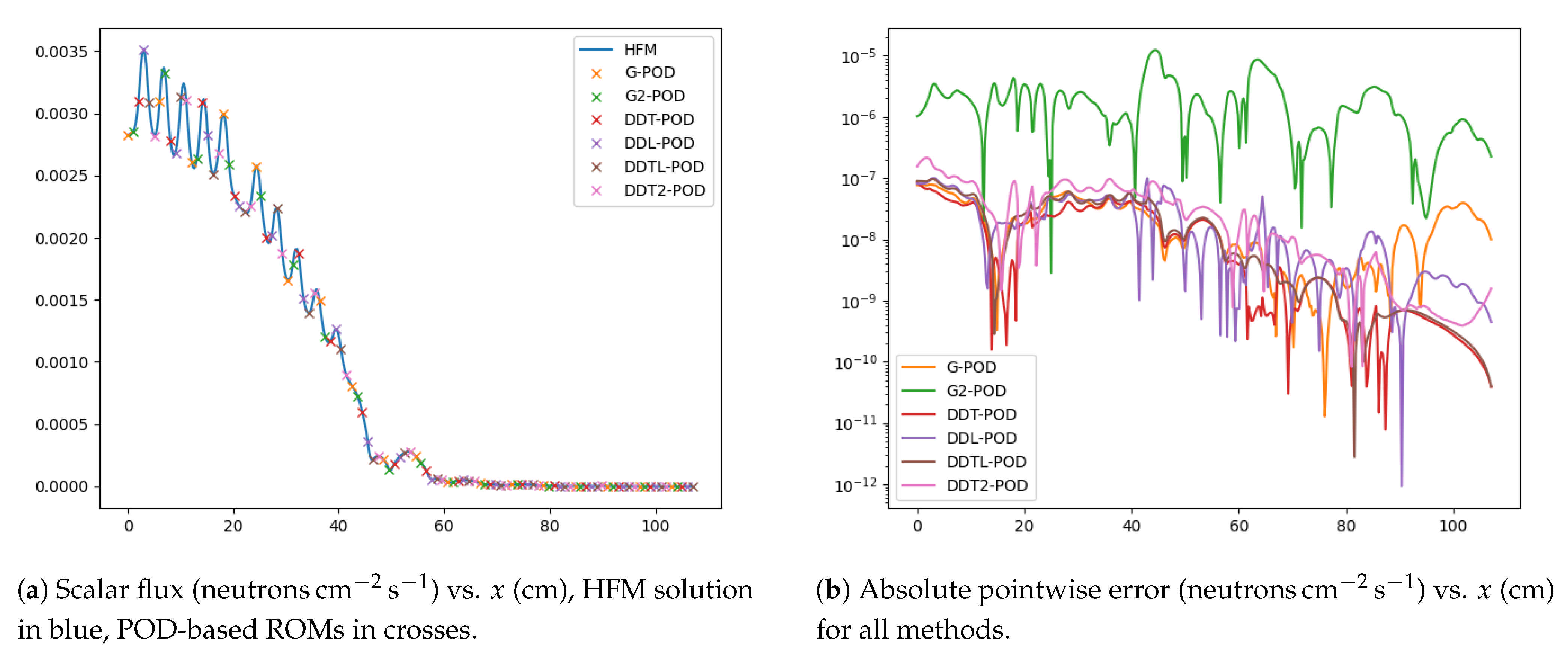
Energies 14 01369 g003
Figure 4. Scalar flux for Energy Group 1 for the HFM (blue) and POD methods and the pointwise error between them with parameters R 1 = 2 , R 2 = 2 , R 3 = 1 , R 4 = 1 , R 5 = 4 .
Energies 14 01369 g004
Figure 5. Scalar flux for Energy Group 5 for the HFM (blue) and POD methods and the pointwise error between them with parameters R 1 = 2 , R 2 = 2 , R 3 = 1 , R 4 = 1 , R 5 = 4 .
Energies 14 01369 g005
Figure 6. Scalar flux for Energy Group 9 for the HFM (blue) and POD methods and the pointwise error between them with parameters R 1 = 2 , R 2 = 2 , R 3 = 1 , R 4 = 1 , R 5 = 4 .
Energies 14 01369 g006
Figure 7. Scalar flux for Energy Group 13 for the HFM (blue) and POD methods and the pointwise error between them with parameters R 1 = 2 , R 2 = 2 , R 3 = 1 , R 4 = 1 , R 5 = 4 .
Energies 14 01369 g007
Figure 8. Scalar flux for Energy Group 17 for the HFM (blue) and POD methods and the pointwise error between them with parameters R 1 = 2 , R 2 = 2 , R 3 = 1 , R 4 = 1 , R 5 = 4 .
Energies 14 01369 g008
Figure 9. Scalar flux for Energy Group 21 for the HFM (blue) and POD methods and the pointwise error between them with parameters R 1 = 2 , R 2 = 2 , R 3 = 1 , R 4 = 1 , R 5 = 4 .
Energies 14 01369 g009
Figure 10. Boxplots showing the errors for all six methods. The median is given by the orange line, the interquartile ranges by the box and the minimum and maximum values by whiskers.
Energies 14 01369 g010
Figure 11. k eff vs. iteration number for the HFM and the three methods with limited (lim) number of snapshots or smart selection of number of basis functions.
Energies 14 01369 g011
Figure 12. Scalar flux for Energy Group 1 for the HFM (blue) and POD-based ROMs, with limited number of snapshots or smart selection of number of basis functions, in crosses, and the pointwise error between them with parameters R 1 = 2 , R 2 = 2 , R 3 = 1 , R 4 = 1 , R 5 = 4 .
Energies 14 01369 g012
Figure 13. Scalar flux for Energy Group 1 for the HFM (blue) and POD-based ROMs, with the limited number of snapshots or smart selection of the number of basis functions, in crosses, and the pointwise error between them with parameters R 1 = 2 , R 2 = 2 , R 3 = 1 , R 4 = 1 , R 5 = 4 .
Energies 14 01369 g013
Figure 14. Scalar flux for Energy Group 1 for the HFM (blue) and POD-based ROMs, with the limited number of snapshots or smart selection of the number of basis functions, in crosses, and the pointwise error between them with parameters R 1 = 2 , R 2 = 2 , R 3 = 1 , R 4 = 1 , R 5 = 4 .
Energies 14 01369 g014
Figure 15. Scalar flux for Energy Group 1 for the HFM (blue) and POD-based ROMs, with the limited number of snapshots or smart selection of the number of basis functions, in crosses, and the pointwise error between them with parameters R 1 = 2 , R 2 = 2 , R 3 = 1 , R 4 = 1 , R 5 = 4 .
Energies 14 01369 g015
Figure 16. Scalar flux for Energy Group 1 for the HFM (blue) and POD-based ROMs, with the limited number of snapshots or smart selection of the number of basis functions, in crosses, and the pointwise error between them with parameters R 1 = 2 , R 2 = 2 , R 3 = 1 , R 4 = 1 , R 5 = 4 .
Energies 14 01369 g016
Figure 17. Scalar flux for Energy Group 1 for the HFM (blue) and POD-based ROMs, with the limited number of snapshots or smart selection of the number of basis functions, in crosses, and the pointwise error between them with parameters R 1 = 2 , R 2 = 2 , R 3 = 1 , R 4 = 1 , R 5 = 4 .
Energies 14 01369 g017
Figure 18. Boxplots showing the errors for methods with the limited number of snapshots and smart selection of the number of basis functions. The median is given by the orange line, the interquartile ranges by the box and the minimum and maximum values by whiskers.
Energies 14 01369 g018
Table 1. Table showing possible domains within a system. The rows represent the material type of domain, and the columns represent the location within the system. UOX, Uranium Oxide; MOX, Mixed Oxide.
12345
UOXYesYesYesYesYes unless 4 = Reflector
MOXYesYesYesYesYes unless 4 = Reflector
ReflectorNoNoNoYesYes
Table 2. Table showing possible systems within the smaller data set. The rows represent the material type of domain, and the columns represent the location and how many domains are used in the solution.
U 3 dom U 2 dom U 1 dom
123 12 1
UOXYesYesYes unless 2 = Reflector YesYes Yes
MOXYesYesYes unless 2 = Reflector YesYes Yes
ReflectorNoYesYes YesNo No
Table 3. Table showing the six methods, how many sets of basis functions are retained and the data from which they are constructed. POD, Proper Orthogonal Decomposition.
NameSets of Basis FunctionsData Used to Construct Basis Functions
G-POD1Global data: U G l o b a l , 250 basis functions retained
G2-POD1Global data: U G l o b a l , 50 basis functions retained
DDT-POD3Type of domain: U U O X , U M O X , U R e f l e c t o r
DDL-POD5Location of domain: U 1 , U 2 , U 3 , U 4 , U 5
DDTL-POD12Location and type of domain: U T y p , L o c
DDT2-POD3Type of domain from alternate data set: U U O X , d o m , U M O X , d o m , U R e f l e c t o r , d o m
Table 4. Mean absolute maximum errors in the flux profile and k eff for solutions using POD-based reduced-order models.
G-PODG2-PODDDT-PODDDL-PODDDTL-PODDDT2-POD
Flux Error1.2286 × 10−32.7860 × 10−21.2391 × 10−31.7601 × 10−31.6563 × 10−31.6593 × 10⁻³
k eff Error2.2952 × 10−54.3557 × 10−32.3154 × 10−52.3901 × 10−52.6866 × 10−55.6589 × 10⁻⁵
Table 5. Mean absolute maximum errors in the flux profile and k eff for solutions using POD-based reduced-order models with the limited number of snapshots and smart selection of the number of basis functions.
G-POD-LimDDT-POD-LimDDL-POD-LimG-POD-BasisDDT-POD-BasisDDL-POD-Basis
Flux Error2.4846 × 10−17.5716 × 10−32.1496 × 10−31.2416 × 10−31.2375 × 10−33.1000 × 10⁻³
k eff Error2.3198 × 10−21.3405 × 10−37.5412 × 10−52.5474 × 10−52.4721 × 10−56.1249 × 10⁻⁵
Publisher’s Note: MDPI stays neutral with regard to jurisdictional claims in published maps and institutional affiliations.

