Evaluation and Optimization of a Two-Phase Liquid-Immersion Cooling System for Data Centers

Abstract

An efficient cooling system for data centers can boost the working efficiency of servers and promote energy savings. In this study, a laboratory experiment and computational fluid dynamics (CFD) simulation were performed to explore the performance of a two-phase cooling system. The coefficient of performance (COP) and partial power usage effectiveness (pPUE) of the proposed system was evaluated under various IT (Information Technology) loads. The relationship between the interval of the two submerged servers and their surface temperatures was evaluated by CFD analysis, and the minimum intervals that could maintain the temperature of the server surfaces below 85 °C were obtained. Experimental results show that as server power increases, COP increases pPUE decreases. In one experiment, the COP increased from 19.0 to 26.7, whereas pPUE decreased from 1.053 to 1.037. The exergy efficiency of this system ranges from 12.65% to 18.96%, and the tank side accounts for most of the exergy destruction. The minimum intervals between servers are 15 mm under 1000 W of power, 20 mm under 1500 W, and more than 30 mm under 2000 W and above. The observations and conclusions in this study can be valuable references for the study of cooling systems in data centers.

1. Introduction

The boosting of digital technology (e.g., Internet of Things, artificial intelligence, big data, 5G, cloud computing) and its extensive applications in many industries, such as transportation [1], communication [2], manufacturing [3], medicine [4], and education [5], demonstrate an increasing need for data processing, storage, and transmission. A data center can be a building or part of a building where data are gathered, processed, and stored [6]. According to a report by the Synergy Research Group, by the end of the third quarter of 2019, there were 504 hyperscale data centers worldwide [7], and another report predicted that this number would increase by 12–14% annually over the next five years [8]. Of all the data centers in 2019, approximately 40% reside in the US, and China, Japan, the UK, Germany, and Australia collectively contain 32%. Data centers typically involve high energy consumption. In the UK, data centers accounted for 1.5% of electricity usage in 2016, with power consumption projected to increase by 20% in 2020 [9]. In China, data centers used 160.8 billion kWh of electricity in 2018, which exceeded the total electricity consumption of all of Shanghai [10].

In addition to power equipment and accessory components, data centers consist of two major energy-consuming parts, IT and heating, ventilation, and air conditioning (HVAC) equipment, which account for approximately 90% of the total energy usage [11]. The HVAC equipment itself has been reported to be responsible for 34% of this total energy [12], because of the need to cool the all-day operation of high-power-density IT equipment and maintain the indoor thermal environment within the appropriate temperature zones [13]. The HVAC system needs to be in operation for approximately 24 h per day. To improve the energy efficiency of a data center, optimizing the HVAC system is one of the key steps. Power usage effectiveness (PUE) is an industry-preferred index for evaluating the infrastructure energy efficiency of data centers [14]. A small PUE approaching 1.0 indicates that the data center approaches optimal energy efficiency.

Data center cooling systems can be classified into two types—air-cooled systems [15,16] and liquid-cooled systems [17]. The first type sends cold air to racks on which servers are placed and then removes the heat generated by the servers. The advantages of this type of system include the following: (1) this traditional air-cooling system is relatively mature and easy to construct and (2) this system has promising potential for the use of free cooling resources, such as natural cold air and water [18], which could substantially benefit the reduction of power usage, decreasing the PUE from a value of 2.01 for a typical computer room air conditioner system to a value as low as 1.1 with free cooling [19,20]. The drawbacks of the air-cooled system are significant, such as a low heat transfer coefficient, difficulty in the design and control of cold and hot air flow, asymmetrical cooling in different servers owing to the geometrical layouts of data centers, large power consumption through the operation of chillers, fans, and pumps, and unstable cooling capacity caused by the outdoor thermal environments [12,17,21,22].

The liquid-cooled system requires the removal of high-density heat, which is too high to be removed by the air-cooled system; This heat is dissipated by high-performance information and communication technology (ICT) devices. Based on the direct contact of the liquid with the heat sources, the liquid-cooled system can be further categorized as direct cooling and indirect cooling. For direct liquid cooling, the dielectric liquid absorbs heat from the electronic components directly; this type of heat transfer can be highly effective [17,23]. Passive two-phase cooling is a fluid-cooled approach in which electronic components are submerged in a phase-changeable liquid bath in a closed box. When the surface temperature of the electronic components exceeds the evaporation temperature of the liquid, the process of boiling heat transfer is triggered, removing the extra heat in the form of vapor bubbles. The produced vapor rises up and further condenses through a water-based condenser installed above the bath. Finally, the heat is absorbed and removed by the coolant; the vapor is then liquefied and drips back to the bath, driven by gravity [24,25]. Compared with the air-cooled system, the two-phase cooling system could reduce the use of accessory equipment, such as chiller pumps and fans, potentially improving the energy efficiency of data centers. In addition, this system could avoid the surface temperature symmetry of electronic devices and guarantee their working environment.

Dashtebayaz and Namanlo [26] studied an air-based cooling system that performs waste heat recovery and reported a coefficient of performance (COP) that varied in the 3–5 range with a PUE of approximately 2.5. Chen et al. [27] applied spray-cooling technology to the cooling of computer centers and suggested that the system COP is highly dependent on the inlet water temperature, with COP possibly changing from 3 to 15 and PUE ranging from 1.45–1.52. Cho et al. [28] proposed many green technologies that can be applied to data center cooling systems under different climatic contexts and determined by applying suitable strategies. The target PUE was in the range of 1.2–1.6. Dong et al. [29] explored the effectiveness of using free-cooling resources to cool data centers and suggested that natural cooling could increase the system COP by 23.7%, rising from 5.9 to 7.3. Lu et al. [30] reported the PUE of data centers in Finland, highlighting its range of variation of 1.2–1.5.

In a two-phase cooling system, the ICT equipment is completely submerged in the dielectric liquid bath; nucleate boiling occurs on the server surface when the server temperature reaches the boiling temperature of the dielectric liquid. Wu et al. [31] evaluated a full-scale two-phase liquid-immersion DC cooling system in a tropical environment. They found that the exergetic efficiency experienced a small rate of decrease, while the supplied power rate increased. The highest efficiency of 69.9% was obtained at zero load, whereas the lowest efficiency of 65.9% was observed at full load. Kanbur et al. [32] studied a two-phase liquid-immersion data center cooling system through experimental and thermo-economic analyses. They found that the optimal COP and PUE values occurred at maximum operation loads of 6.67 and 1.15, respectively, whereas the minimum COP and highest PUE were observed at the minimum operation loads of 2.5 and 1.4, respectively. Choi et al. [33] used two-phase cooling (HFE-7100) for a polymer electrolyte membrane fuel cell. They found that the two-phase boiling heat transfer coefficients of the HFE-7100 in mini-channels were strongly dependent on heat flux and vapor quality but less sensitive to mass flux. However, at present, there are fewer research reports on the mining machine motherboard of the two-phase liquid-immersion cooling system.

Computational fluid dynamics (CFD) simulations have been widely applied to validate the performance of specific cooling systems for data centers and to present optimal designs based on the detailed results of the simulations. Ahmadi et al. [34] verified the energy-saving potential, optimal designs, and operation conditions for the computer room air handling bypass method in cooling data centers by using CFD simulations. Hassan et al. [35] performed CFD simulations in ANSYS Fluent and obtained the temperature, airflow, and pressure distributions for a data center. The prediction provided a three-dimensional (3D) thermal map of the data center and helped to optimize the cooling system. Fulpagare et al. [36] explored transient CFD models to simulate the dynamic requirements of cooling systems to achieve smart control in data centers, and the model performance was validated based on experiments. Using CFD simulations, Nada et al. [37] studied the performance of data centers under different configurations and summarized the effects of the computer room air conditioning unit layout on the thermal performance of the racks. Most previous CFD studies have focused on air-cooled systems; however, studies that focused on two-phase cooling systems are scant. Cheng et al. [38] studied a single-phase immersion cooling system (using 3 M Novec 7100) for single CPU cooling via 3D numerical analysis using ANSYS Fluent. The results of the simulations showed that there was an unbalanced heat distribution around the CPU, and higher flowing speeds of the liquid coolant led to the removal of more heat, resulting in lower CPU temperatures and more balanced heat distribution around the CPU. Ali et al. [39] numerically investigated the thermal performance and stress analysis of enhanced copper spreaders for nucleate boiling immersion cooling of high-power electronic chips. An et al. [40] developed a 3D numerical model using ANSYS Fluent to study two-phase immersion cooling for electronic components. They found that Novec 7000 can support cooling a 5 cm × 5 cm heat source in a vertical orientation with power as high as 225 W (heat flux of 9 W/cm²). However, less research was reported using CFD simulation to study the arrangement of the server motherboards.

This study consisted of experiments and a series of CFD simulations. First, an innovative cooling structure and procedure for a two-phase immersion cooling system were developed. Six different cases were investigated to analyze the thermal management performance in the operational load range of 1127–1577 W. The energy efficiency of the system was evaluated based on the partial power usage effectiveness (pPUE) and COP indices, and exergy analysis was performed. Finally, an arrangement of submerged servers was proposed by CFD simulation. This study aimed to formulate an innovative two-phase immersion cooling system for data centers, which includes an optimal arrangement of the servers. Data from the two-phase cooling system were collected; the results and conclusions presented herein may potentially serve as valuable references for researchers and engineers.

2. Methodology

2.1. Experimental Study

A novel, innovative cooling structure and procedure of a two-phase immersion cooling system were established for the cooling of ICT devices. The scheme of the proposed two-phase cooling system is shown in Figure 1, which includes a primary heat exchanger and a tank with coolant and server boards as ICT devices. The ambient air temperature was maintained at 21–23 °C.

Figure 2a shows the tank where real servers were submerged in the dielectric liquid Novec 7100 supplied by 3M (Minnesota Mining and Manufacturing, Saint Paul, MN, USA) [41]. The dielectric liquid, being expensive, was filled in the tank only to submerge all the servers (Figure 2c) during the experiments. For each experiment, the server power output was maintained at a constant level. As the surface temperature of the servers rose and reached the boiling point of Novec 7100, the surrounding liquid formed bubbles and absorbed heat through evaporation. The produced vapor gathered on the top of the tank, where condenser coils were placed around the wall, as shown in Figure 2c. The heat was transferred from the vapor to the cold coolant circulating inside the condenser coils and was removed from the tank. Thereafter, the vapor condensed into the fluid phase and dripped back onto the liquid bath because of gravity. The heated coolant inside the coil released heat to the environment by a primary heat exchanger, as shown in Figure 2d.

Table 1. Properties of Novec 7100 at 25 °C.

Boiling Point (°C)	Vapor Pressure (kPa)	Molecular Weight (g/mol)	Density Liquid (kg/m3)	Dynamic Viscosity (cSt)	Specific Heat (J/kgK)
61	27	250	1510	0.38	1183

lists the thermal characteristics of Novec 7100 at 25 °C, and the specific data are listed in

Table A1. The thermal properties of Novec 7100.

Temperature (°C)	Density (kg/m3)	Viscosity (m2/s)	Dynamic Viscosity (kg/m s)	Kinematic Viscosity (m2)/s)	Specific Heat (J/kg K)	Thermal Conductivity (W/m K)	Saturated Vapor Pressure(Pa)
−90	1825.19	6.04 × 10−6	0.0110	11.025	953	0.0913	12.904
−80	1798.27	3.64 × 10−6	0.0065	6.542	973	0.0893	35.987
−70	1771.35	2.44 × 10−6	0.0043	4.319	993	0.0873	90.718
−60	1744.43	1.76 × 10−6	0.0030	3.075	1013	0.0854	209.684
−50	1717.51	1.35 × 10−6	0.0023	2.310	1033	0.0834	449.593
−40	1690.59	1.07 × 10−6	0.0018	1.803	1053	0.0815	902.934
−30	1663.67	8.7 × 10−7	0.0014	1.446	1073	0.0795	1712.302
−20	1636.75	7.24 × 10−7	0.0011	1.185	1093	0.0776	3087.064
−10	1609.83	6.14 × 10−7	0.0009	0.988	1113	0.0756	5321.763
0	1582.91	5.28 × 10−7	0.0008	0.835	1133	0.0737	8815.499
10	1555.99	4.6 × 10−7	0.0007	0.715	1153	0.0717	14,091.424
20	1529.07	4.05 × 10−7	0.0006	0.619	1173	0.0698	21,815.442
30	1502.15	3.61 × 10−7	0.0005	0.542	1193	0.0678	32,813.298
40	1475.23	3.24 × 10−7	0.0004	0.478	1213	0.0658	48,085.294
50	1448.31	2.94 × 10−7	0.0004	0.426	1233	0.0639	68,818.070
60	1421.39	2.69 × 10−7	0.0003	0.383	1253	0.0619	96,393.020
70	1394.47	2.49 × 10−7	0.0003	0.346	1273	0.0600	132,391.102

in Appendix A. The dimensions of the tank were 650 × 450 × 1050 mm³ (length × width × height), and the tank was insulated to prevent the influence of the surrounding thermal environment. The servers used in this study were application-specific integrated circuit (ASIC) miners designed to “mine” a specific cryptocurrency. The type of server board was T2T-25T, and the dimensions of each board were 235 × 182 × 8 mm³. There were 140 T2T CPUs on each board, and the dimensions of the CPU were 8 × 8 × 1 mm³, with an average CPU TDP of 8.37 W/cm². The server boards were placed at 100 mm intervals. This type of server has several modes with rated power outputs ranging from 1000 to 2000 W. The mode of each server can be controlled remotely through a computer program.

During the experiment, all the data were measured when the system was under a stable status, characterized by a lack of fluctuations in the CPU surface temperature. Under each condition, the system was kept running for 60 min before the data were recorded. The temperatures of the server surface, liquid bath, and inlet and outlet coolant inside the coils were recorded using a digital temperature controller (E5CC, OMRON, Kyoto, Japan). The temperature was measured using K-type thermocouples (TT-K-24, OMEGA, Norwalk, CT, USA), which were calibrated using a mercury thermometer with an accuracy of ±0.1 °C. The core temperature of the servers was measured and recorded automatically by the aforementioned computer program. The pressure in the tank was monitored by an automatic pressure relief valve with a pressure sensor (ZSE40AF-01-T, SMC, Kyoto, Japan), with the pressure set to 1.2 kg/cm². The heat from the coolant was removed by a heat exchanger (ERM-3K3UC Liquid Cooling System, Koolance, Auburn, AL, USA), and the cooling capacity of the cooling system was 2600 W (8872 BTU/h). The power of the cooling unit (including the pump and the fan) was monitored using a power meter that can monitor and record real-time power consumption. The experiment consisted of six conditions, and the stable data are listed in

Table 2. Operating conditions and experimental results.

Case	Room Temperature (°C)	CPU Power(W)	Heat Exchanger Coolant Temperature (°C)		Temperature of CPU (°C)
			Inlet	Outlet	Surface	Core
1	21.9	1127	26.5	25.1	66.0	67.4
2	21.6	1396	27.1	25.8	68.8	71.2
3	22.4	1332	27.9	26.5	68.5	70.7
4	23.0	1494	29.2	27.6	70.5	72.3
5	23.3	1516	29.6	28.1	71.7	72.9
6	23.4	1577	30.1	28.4	71.9	73.3

.

2.2. CFD Simulation

2.2.1. Physical Model and Boundary Conditions

In this study, a commercial CFD tool, ANSYS Fluent, was used to complete the simulation [42]. CFD simulations were intended to explore the effects of the interval of adjacent servers on the performance of a two-phase cooling system and propose an appropriate server arrangement. The assumption is that for a given power of servers and a specific cooling setting, there is the shortest interval between submerged servers for which each server should run in an ideal environment with core temperatures lower than the requirements. The purpose of searching for the shortest interval is that the submerged space in a two-phase cooling tank is limited; thus, a well-arranged matrix of servers facilitates efficient usage of space, thereby providing savings in investment and running costs.

Building physical models is the first step in running a CFD simulation. The dimensions of the simulated two-phase cooling tank are the same as those used in the experimental study, which is 650 × 450 × 1050 mm³ (L × W × H), as demonstrated in Figure 3. Figure 3b shows the mesh distribution near the server board, which was locally encrypted. The walls of the tank were set as adiabatic, and three server boards were placed under a 50 mm liquid bath, with the dimensions of each board at 235 × 182 × 8 mm³ (L × W × H). There are 140 CPUs on each board, and each CPU has dimensions of 8 × 8 × 1 mm³. During the simulation, the boundary conditions of the servers were set as constant heat flow, which was consistent with the server power output. There are some assumptions and simplifications in this model. The server boards, including printed circuit boards and CPUs (covered with phenolic epoxy resin), were treated as an entire heating plate covered with phenolic epoxy resin (thermal conductivity of 2.2 W/m K). The coolant-side cooling equipment and heat transfer process were removed from the simulation, and the top of the tank was considered as a pressure outlet. The assumption was that all the heat from the vapor could be fully released to the environment by the heat exchanger. These simplifications were applied because this simulation focused on the heat transfer between the submerged servers and the liquid but not on the entire system. The grid chosen in this study was “Tet/Hybrid,” which consisted of tetrahedrons and other hybrid elements. One of the limitations of the model is that the detail of the CPU was ignored.

2.2.2. CFD Modeling of Boiling Flow

In this study, a volume of the fluid model was used to simulate the boiling heat transfer (two-phase vapor–liquid flow regimes) in the tank. In this multiphase flow model, an Eulerian–Eulerian approach is applied, where both fluids are assumed to behave as continuous media [43]. The mass and energy transfer between both phases during the evaporation process, as shown in Equations (1)–(3) (Reynolds-averaged Navier–Stokes (RANS) equations), and further details on these equations were provided by Versteeg g [44].

$$\frac{\partial }{\partial t}(\rho )+{\displaystyle \sum _{j=1}^3\frac{\partial }{\partial x_i}}\left(\rho {\overline{u}}_i\right)=S_M$$

(1)

$$\frac{\partial }{\partial t}\left(\rho {\overline{u}}_i\right)+{\displaystyle \sum _{j=1}^3\frac{\partial }{\partial x_j}}\cdot \left(\rho {\overline{u}}_i{\overline{u}}_j\right)=-\frac{\partial p}{\partial x_i}+{\displaystyle \sum _{j=1}^3\frac{\partial }{\partial x_j}}\left[\mu \left(\frac{\partial {\overline{u}}_i}{\partial x_j}+\frac{\partial {\overline{u}}_j}{\partial x_i}-\frac{2}{3}{\delta }_{ij}{\displaystyle \sum _{l=1}^3\frac{\partial {\overline{u}}_l}{\partial x_l}}\right)\right]+{\displaystyle \sum _{j=1}^3\frac{\partial }{\partial x_j}}\left(-\rho \overline{u_i^{\prime }{u}_j^{\prime }}\right)+S_{F,i}$$

(2)

$$\frac{\partial }{\partial t}(\rho E)+{\displaystyle \sum _{j=1}^3\frac{\partial }{\partial x_j}}\left(\rho E{\overline{u}}_j\right)={\displaystyle \sum _{i=1}^3{\displaystyle \sum _{j=1}^3\left(\frac{\partial }{\partial x_j}\left({\tau }_{ij}-\rho \overline{u_i^{\prime }{u}_j^{\prime }}\right){\overline{u}}_i\right)}}-{\displaystyle \sum _{j=1}^3\frac{\partial }{\partial x_j}}{q}_j+S_E$$

(3)

where S_M is the source term in the mass conservation equation (kg/m³ s), S_F is the source term in the momentum conservation equation (kg/m² s²), and S_E is the source term in the energy equation (J/m³ s).

The RANS equations describe the transport of the averaged flow quantities in which the entire range of turbulence scales is modeled. Because of the averaging, these equations contain additional unknown variables called Reynolds stresses. By applying the Boussinesq hypothesis [44], the Reynolds stresses are related to the mean velocity gradients. The expression for the calculation of these Reynolds stresses corresponds to Equation (4).

$$-\rho \overline{u_i^{\prime }{u}_j^{\prime }}={\mu }_{turb}\left(\frac{\partial {\overline{u}}_i}{\partial x_j}+\frac{\partial {\overline{u}}_j}{\partial x_i}\right)-\frac{2}{3}\left(\rho k+{\mu }_{turb}{\displaystyle \sum _{l=1}^3\frac{\partial {\overline{u}}_l}{\partial x_l}}\right){\delta }_{ij}$$

(4)

To solve this equation, an expression for the turbulent viscosity (µ_turb) is required. The calculation of turbulent viscosity using the standard k‒ε model is computationally expensive. In the first step, two additional transport equations for the turbulent kinetic energy k and the viscous dissipation of the turbulent kinetic energy ε are solved, which correspond with Equations (5) and (6). Finally, the turbulent viscosity is calculated as a function of k and ε (Equation (8)).

$$\frac{\partial }{\partial t}(\rho k)+{\displaystyle \sum _{j=1}^3\frac{\partial }{\partial x_j}}\left(\rho k{\overline{u}}_j\right)={\displaystyle \sum _{j=1}^3\frac{\partial }{\partial x_j}}\left[\left(\mu +\frac{{\mu }_{\mathrm{turb} }}{{\sigma }_k}\right)\frac{\partial k}{\partial x_j}\right]+{\overline{P}}_k-\rho \epsilon$$

(5)

$$\frac{\partial }{\partial t}(\rho \epsilon )+{\displaystyle \sum _{j=1}^3\frac{\partial }{\partial x_j}}\left(\rho \epsilon {\overline{u}}_j\right)={\displaystyle \sum _{j=1}^3\frac{\partial }{\partial x_j}}\left[\left(\mu +\frac{{\mu }_{\mathrm{turb} }}{{\sigma }_{\epsilon }}\right)\frac{\partial \epsilon }{\partial x_j}\right]+C_{1\epsilon }\frac{\epsilon }{k}{\overline{P}}_k-C_{2\epsilon }\rho \frac{{\epsilon }^2}{k}$$

(6)

$${\overline{P}}_k={\displaystyle \sum _{i=1}^3{\displaystyle \sum _{j=1}^3\left[\left({\mu }_{\mathrm{turb} }\left(\frac{\partial {\overline{u}}_i}{\partial x_j}+\frac{\partial {\overline{u}}_j}{\partial x_i}-{\delta }_{ij}{\displaystyle \sum _{l=1}^3\frac{2}{3}}\frac{\partial {\overline{u}}_l}{\partial x_l}\right)-\frac{2}{3}\rho k{\delta }_{ij}\right)\frac{\partial {\overline{u}}_j}{\partial x_i}\right]}}$$

(7)

$${\mu }_{\mathrm{turb}}=\rho C_{\mu }\frac{k^2}{\epsilon }$$

(8)

Many expressions describing the mass transfer during evaporation are based on gas kinetic theory. A well-known equation for the net mass flux over the vapor–liquid interphase during the evaporation process is the following Hertz–Knudsen equation [45]:

$$J^{\prime }={\alpha }_{\mathrm{c}}\frac{\sqrt{M}}{\sqrt{2\pi R}}\left(\frac{p}{\sqrt{T_{\mathrm{v}}}}-\frac{p_{\mathrm{sat}}\left(T_{\mathrm{l}}\right)}{\sqrt{T_1}}\right)$$

(9)

where J is the net mass flux over the vapor–liquid interface (kg/m² s), α_c is the accommodation coefficient, M is the molecular weight (kg/kmol), T_v is the temperature of the vapor phase (K), T_l is the temperature of the liquid phase (K), and p_sat is the saturation pressure (P_a). In the case of condensation, αc is defined as the ratio of the experimentally observed condensation velocity to the maximal theoretical condensation velocity. Meanwhile, in the case of evaporation, this parameter is defined as the ratio of the experimentally observed evaporation velocity to the maximal theoretical evaporation velocity [43]. The specific calculation procedure for the mass and energy transfer during the evaporation process was based on the study by Schepper et al. [43].

The semi-implicit method for pressure-linked equations (SIMPLE) algorithm was used for pressure–velocity coupling. A body force-weighted scheme was used to discretize the pressure terms. The momentum, energy transport, and turbulence equations were solved using the quadratic upstream interpolation for the convective kinematics (QUICK) scheme. The convergence criteria of the whole solution were defined with respect to the residuals for mass, momentum, turbulence, and energy––10⁻³ for the mass, momentum, and turbulence residuals and 10⁻⁶ for energy residual.

Table 3. Settings of the computational fluid dynamics (CFD) Model.

Setting Parameters	Type	Settings/Options
Solver type		Pressure-based
Turbulence model		k–ε realizable model
Near-wall treatment		Standard wall functions
Pressure-velocity coupling scheme		SIMPLE
Spatial discretization	Gradient	Least-squares cell-based
	Pressure	Body force-weighted
	Momentum	QUICK
	Turbulent kinetic energy (k)	QUICK
	Turbulent dissipation rate (ε)	QUICK
	Energy	QUICK
Residuals	Continuity	0.001
	X, Y, Z-Velocity	0.001
	Energy	10−6
	k, ε	0.001

shows a summary of the applied CFD model settings.

2.2.3. Material Properties

The thermodynamic properties of the liquid and vapor were obtained from the Novec 7100 manual [41]. Each thermodynamic parameter was approximated by temperature-dependent polynomial functions. Figure 4 and Figure 5 provide two examples that show the correlations between the temperature and the liquid dynamic viscosity/vapor conductive coefficient.

Table A2. Thermodynamic properties of the Novec 7100 (vapor and liquid).

Physical Parameters	Liquid	Vapor
Density (kg/m3)	y = − 2.692T + 1582	y = 0.0034T2 − 0.103T + 2.337
Specific heat (J/kgK)	y = 2T + 1133	y = 216.4 + 4.749T + 0.00144T2 + 4.265 × 10−6T3 + 1.758 × 10−9 T4
Conductive coefficient	y = − 0.00027T + 0.073	y = 0.01293 + 4.74 × 10−5T
Dynamic viscosity (kg/m s)	y = 4 × 10−5T4 − 1 × 10−7T3 + 2 × 10−7T2 –1 × 10−5T + 0.0008	y = 8.294 × 10−4 − 1.15 × 10−5T + 6.75 × 10−8T2

in Appendix A lists all the temperature-dependent properties of the thermodynamic parameters used in Fluent.

2.2.4. Grid Independence

The analysis of the grid independence was conducted by running simulations with different numbers of grid cells, as shown in

Table 4. Analysis of grid independence.

Cell Number	Time Step (s)	Mean Surface Temperature (°C)	Temperature Difference (%)
121,471	0.01	72.65	-
246,680	0.01	72.28	−0.5%
510,438	0.01	71.63	−0.9%

. The time step (∆t) was 0.01 s, and the maximum number of iterations was 20. The total number of time steps was 5000 (total physical time 50 s), which was sufficient to obtain steady-state conditions, and the calculation time was nearly 23 h for one case. The initialization temperature was 331 K, and the vapor volume fraction was 0. A computer (Thinkpad S3, i5-4210U, two cores, four threads, Lenovo, Peking, China) with Windows 7 Home Edition was used for the simulations. The mean surface temperature of the servers was taken as a comparative index, and the results showed that the predicted surface temperature with 510,438 cells changed by only 0.9%, with the corresponding temperature predicted with 121,471 cells. In the following simulations, the grid setting of 121,471 cells was selected.

2.2.5. CFD Model Validation

To begin the study, model validation was performed by comparing the experimental results, as displayed in

Table 5. Verification of the proposed CFD settings.

Power (W)	Experimental Average Surface Temperature (°C)	Numerical Average Surface Temperature (°C)	Error (%)	Numerical Heat Transfer Coefficients (kW/m2 K)	Experimental Average Liquid Temperature (°C)	Numerical Average Liquid Temperature (°C)
1127	66.0	69.43	4.95	7.98	58.5	61.40
1332	68.5	71.56	4.28	10.16	61.5	64.13
1577	71.9	74.67	3.71	10.46	63.8	66.17
Ref. [43]	-	-	-	6.1 − 18.5 (∆T = 10 °C)

. In summary, the maximum error was found to be less than 5%, which implies that the CFD simulation precision reached the level of the experiment. The heat transfer coefficients of HFE-7100 were assessed for the interval between every two servers ∆l = 100 mm under different powers. The results showed that the heat transfer coefficients in our study were within a reasonable range compared with those demonstrated in other studies [46].

2.3. COP and pPUE

COP and PUE are two important indices used to evaluate the system energy performance. COP is defined as the ratio of cooling energy removed by a cooling system to the consumed power [47]. With the assumption of all the input server power transferring to heat, in this case, COP can be represented by Equation (10).

$$COP=\frac{W_{server}}{W_{total}}$$

(10)

where W_server is the server power and W_total is the total cooling power consumption in units of W.

PUE is used to assess the thermal performance of cooling systems in data centers and is recommended by ASHRAE (American Society of Heating, Refrigerating and Air-Conditioning Engineers). In this study, owing to the two-phase immersion cooling system, a component of the real ICT equipment cooling system. Therefore, the pPUE was used to assess the efficiency of the two-phase immersion cooling system. It is defined as the total energy within a boundary divided by the IT equipment energy within that boundary (pPUE can only be calculated for zones with IT) [48]. Theoretically, pPUE should be larger than 1.0, and a value close to 1.0 implies high energy efficiency. The pPUE, in this case, can be calculated using Equation (11).

$$pPUE=\frac{W_{total}+W_{server}}{W_{server}}$$

(11)

2.4. Exergy Analysis

Exergy analysis is based on the second law of thermodynamics and is an important method to evaluate the efficiency of a cooling system [49,50,51]. The specific exergy flow in any state can be expressed as

$$e_f=h-h_0-T_0\left(s-s_0\right)$$

(12)

where h is the specific enthalpy, kJ/kg; s is the specific entropy, kJ/(kg K); and “0” represents the reference state of T = 293.15 K.

The exergy efficiency can be defined as the ratio, as shown in Equation (13). For each part of the exergy destruction (${\dot{E}}_{D,i}$), its percentage can be calculated using Equation (14).

$$\eta =1-\frac{{\dot{E}}_D}{W_{\mathrm{total}}}$$

(13)

$$p_{d,i}=\frac{{\dot{E}}_{D,i}}{{\dot{E}}_D}$$

(14)

The transfer of heat in the proposed two-phase cooling system is accompanied by exergy destruction owing to an increase in entropy. On the tank side, the exergy destruction results from the evaporation of the liquid bath by absorbing heat from the servers, E_d,1 and condensation of the vapor through the loss of heat to the coolant inside the coils, E_d,2. The heat received by the coolant from the condensed vapor, E_d,3, is released to the environment through a heat exchanger, E_d,4.

When the liquid bath is heated and evaporated to gas, the exergy destruction E_d,1 is calculated as

$$E_{d,1}=W_{\mathrm{server}}+m_l\left(e_{f,l}-e_{f,g}\right)$$

(15)

where m_l is the mass flow of the evaporated liquid (kg/s), e_f,l is the specific exergy rate of the liquid (kJ/kg), and e_f,g is the specific exergy rate of the vapor, kJ/kg.

When the evaporated gas is condensed to the liquid phase by the condenser, the exergy destruction E_d,2 is calculated as

$$E_{d,2}=m_g\left(e_{f,g}-e_{f,l}\right)-\left(1-\frac{T_0}{T_l}\right)Q_1$$

(16)

$$Q_1=m_g\left(h_g-h_l\right)$$

(17)

where T₀ is the setpoint temperature. In this study, the temperature was set as the ambient temperature 293.15 K, T_l is the temperature of the condensed liquid near the servers, K; Q₁ is the resealed heat of vaporization under relatively stable conditions, W; and m_g is the mass flow of condensed gas (kg/s).

When the coolant is heated by the evaporated gas, the exergy destruction E_d,3 is calculated as

$$E_{d,3}=m_w({\mathrm{e}}_{\mathrm{f},\mathrm{w},1}-{\mathrm{e}}_{\mathrm{f},\mathrm{w},2})+\left(1-\frac{{\mathrm{T}}_0}{{\mathrm{T}}_{\mathrm{w},\mathrm{l},2}}\right){\mathrm{Q}}_2+{\mathrm{W}}_{\mathrm{pump}}$$

(18)

$$Q_2=m_w\left(h_{w,l,2}-h_{w,l,1}\right)$$

(19)

where T_w,1,2 denotes the temperature of the output coolant (K), Q₂ is the absorbed heat of the coolant (W); m_w is the mass flow of coolant (kg/s); e_f,w,1 denotes the exergy rate of the input coolant; e_f,w,2 denotes the exergy rate of the output coolant, kJ/kg; h_w,l,1 is the enthalpy of the input coolant to the condenser; and h_w,l,2 is the enthalpy of the output coolant to the condenser, kJ/kg. W_pump is the power of the water pump, W.

When the coolant is cooled by the external heat exchanger, the destruction of exergy E_d,4 is

$$E_{d,4}=m_w\left(e_{f,w,2}-e_{f,w,3}\right)-\left(1-\frac{T_0}{T_{w,l,3}}\right)Q_3-W_{hx}$$

(20)

$$Q_3=m_w\left(h_{w,l,2}-h_{w,l,3}\right)$$

(21)

where T_w,l,3 is the temperature of the coolant in the heat exchanger, K; Q₃ is the released heat of the coolant, W; e_f,w,3 is the exergy rate of coolant from the heat exchanger, kJ/kg; and h_w,l,3 is the enthalpy of the coolant from the heat exchanger, kJ/kg, where W_hx is the power of the heat exchanger, W.

The total destruction of exergy is the sum of the above components, written as Equation (22).

$$E_d=E_{d,1}+E_{d,2}+E_{d,3}+E_{d,4}$$

(22)

3. Results and Discussion

3.1. COP and pPUE

Table 6. Operation values under six conditions.

Case	Wserver (W)	Wfan+pump (W)	hf,l (kJ/kg)	sf,l (kJ/kg K)	hf,g (kJ/kg)	sf,g (kJ/kg K)	hf,w,1 (kJ/kg)	sf,w,1 (kJ/kg K)	hf,w,2 (kJ/kg)	sf,w,1,2 (kJ/kg K)
1	1127	59.2	114.120	0.407	228.943	0.749	105.286	0.367	111.558	0.387
2	1396	59.4	114.120	0.407	229.802	0.750	108.631	0.376	113.649	0.394
3	1332	59.1	114.120	0.407	231.090	0.753	111.558	0.386	116.994	0.405
4	1494	59.0	114.120	0.407	231.520	0.753	116.158	0.402	122.430	0.423
5	1516	59.0	114.120	0.407	232.379	0.755	117.621	0.408	124.102	0.429
6	1577	59.0	114.120	0.407	233.238	0.756	119.503	0.412	126.193	0.436

lists the power outputs of servers and the “fan + pump” under six conditions. The server power varies between 1127 W and 1577 W, whereas the power of the “fan + pump” changed only a little because either the pump or the fan was set at the same level under these conditions. Figure 6 shows the results of COP and pPUE calculated from the experimental study. COP ranges from 19.0 to 26.7 and maintains an increasing trend, with the highest value, 26.7, obtained for a power of 1577 W. Meanwhile, pPUE ranges from 1.037 to 1.053 and indicates an opposite trend—the highest value is obtained at a power of 1127 W. The reason for the observed monotonous relationships is that the server power used in this study did not exceed the upper limit of the system cooling capacity. During the study, the power of the fan and water pump was maintained stable at approximately 59.0 W. This allowed the external heat exchanger to release the heat dissipated by the servers efficiently. Thus, there remains the potential for a higher COP or lower pPUE if the server operates at higher power.

By comparing the performances of COP and pPUE, the two-phase cooling system in this study appears to exhibit substantially better energy efficiency than many reported cooling systems or strategies for data centers. The boiling heat transfer involving phase changes could remove heat away from the CPU by a small mass flow of vapor. By comparison, the air-cooling system generally has a lower convective heat transfer coefficient, and to compensate for this, a high-volume airstream is needed, which requires fans to provide a significant amount of power, thus consuming more energy. The second reason is that there is no chiller in the system; thus, considerable energy is conserved. Unlike many air-cooling systems with a chiller, this system does not need compressed refrigerants to remove heat but rather uses circulated coolant to cool the tank. Except for the servers, the only energy-consuming components in this system are the fan and pump. In addition, the outlet coolant temperature can be considerably high, which allows the supply of high-quality waste heat to be further used to enhance the efficiency of the entire system.

3.2. Exergy Analysis

Table 6 lists enthalpy and entropy values of the media in the two-phase cooling system, which were used to calculate the exergy balance equations. The calculated destructions of exergy are presented in

Table 7. Exergy destruction under six cases.

	Power (W)	Ed,1 (W)	Ed,2 (W)	Ed,3 (W)	Ed,4 (W)	Ed	Exergy Efficiency (%)
Case 1	1127	864.91	19.8	27.27	14.28	926.26	18.96%
Case 2	1396	1092.95	19.54	74.99	45.64	1233.12	15.24%
Case 3	1332	1038.41	29.85	70.79	38.37	1177.42	12.65%
Case 4	1494	1163.08	37.61	45.91	60.92	1307.52	13.41%
Case 5	1516	1176.93	46.45	33.15	31.86	1288.39	15.90%
Case 6	1577	1190.93	56.82	107.42	33.01	1388.18	12.86%
Ref. [30]	1150	-	-	-	-	-	18.94%

, and Figure 7 indicates the exergy efficiencies of the proposed two-phase cooling system under six experimental conditions. The exergy efficiency ranges from 12.65% to 18.96%, with an average of 14.84%. Kanbur [32] also analyzed exergy data from a two-phase cooling system and found the average exergy efficiency to vary from 7.9% to 18.9%. The differences between our study and that of Kanbur can be because the room temperature present during the operations in the study by Kanbur was 3–5 °C higher than that in ours. As stated in their study, the operating temperature can affect the heat transfer of the system and, therefore, influence the exergy efficiency. Díaz [52] computed the exergetic efficiency of a typical air-cooled system for data centers, finding an upper limit of approximately 12% for the exergetic efficiency, which was approximately 3% lower than the value in our study. Relatively less total power input can be one of the reasons for the higher exergy efficiency of the two-phase cooling system. In this cooling system, there is no chiller to cool the air; thus, no large fans are used to circulate the air. This results in notable energy and exergy savings, as previous studies have suggested that chillers account for a large part of energy consumption and exergy destruction in the air-cooled system [49]. In addition, the two-phase cooling system involves fewer instances of heat transfer, compared with that in the air-cooled cooling system, which also helps reduce exergy destruction induced by heat transfer. Another advantage of the two-phase cooling system is that it can produce high-quality waste heat, which can be further used to promote the energy efficiency of the entire system. Due to the high boiling point of the phase-changeable liquid (as high as 61 °C), the output temperature of the coolant leaving the tank can theoretically approximate 61 °C, which could lead to a high-quality stream of exergy. This type of waste energy can be directly used as a heat source to supply heat or produce cooling energy through an absorption refrigeration system. Meanwhile, for a typical air-cooled system in a data center, the hot aisle temperature is generally near 35 °C [53], which is relatively lower than that of the proposed two-phase cooling system, limiting the further reuse of its waste heat.

The COP of the proposed two-phase cooling system in this study is generally 4–23 units higher than the values reported in the above references, and pPUE in this study is also the lowest among the reported values. Two reasons contribute to the high energy efficiency of the proposed two-phase cooling system. First, the heat transfer efficiency of immersed cooling is significantly higher than that of many traditional systems, such as air-cooling systems [54]. Meanwhile, there are some similarities between these two types of cooling systems. In this study, the exergy analysis indicates that the tank side contributes nearly 90% of the total exergy destruction, whereas, in an air-cooled cooling system, most of the exergy loss occurs at the chiller side [49]. Although there is no chiller in the two-phase cooling system, the tank itself can be considered as a location where servers are “chilled.” Therefore, a large amount of exergy destruction results; this indicates that the tank-side or server-side modification should be first considered for the optimization of the two-phase cooling system and improvement of its exergy efficiency. Based on experimental results and theoretical analysis, the dominant heat transfer mechanism of HFE-7100 in mini-channels was determined to be nucleate boiling.

3.3. Simulation Results

The thermal maps for the server boards (with a power of 1577 W) are shown in Figure 8a. As the thermal map shows, there is a significant hotspot on the upper server board. Figure 8b shows the temperature distribution on the second server board. From the thermal maps, the heat transfer is not uniform in the vertical direction, and hot spots can occur in the top region because boiling occurs during the heat transfer. The heat transfer behavior during the boiling process is shown in Figure 9. As the temperature of the server board increased, the coolant near the wallboard was heated. Evaporation occurs when the coolant is overheated (T ≥ T_coolant + ∆T), quickly expanding the small bubble near the board. Most of the bubbles grow and reach the interface, where surface evaporation occurs (T > T_boiling). Some of the bubbles in the liquid condense near the coolant (T ≤ T_boiling). Finally, the steam condensed near the top condenser coils (T ≤ T_boiling).

Figure 10 shows the predicted surface temperatures of the servers under different powers and interval settings. The power of the servers was set at five different levels, i.e., 500 W, 1000 W, 1500 W, 2000 W, and 2500 W. The interval between every two servers was ∆l, as shown in Figure 3, and set to 10 mm, 15 mm, 20 mm, 25 mm, and 30 mm. The box plots show distributions of the server surface temperatures, and different colors suggest values under different power levels. Generally, in a specific interval setting, a higher power rate leads to higher surface temperatures. For example, when servers were placed in an interval of 10 mm, the average surface temperatures under an output power of 2500 W were 14.0 °C, 21.3 °C, 31.3 °C, and 42.4 °C higher than the average surface temperatures under output powers of 2000 W, 1500 W, 1000 W, and 500 W, respectively. The same change trend can also be seen in the other four figures with different interval settings. This is because high powers bring more heat flux dissipated from servers to the liquid bath; if the space between the servers is too narrow, a mass of bubbles is produced, accumulating near the servers, and thus restricting the generation of new bubbles. Therefore, the cooling capacity of the liquid bath in a phase change may not be consistent with the output of the servers, causing an increase in the surface temperature. The results from CFD simulations indicate that widening the interval between the servers could help reduce the server temperature.

Figure 11 demonstrates the correlations between the server power and surface temperatures at various intervals. The surface temperatures shown in this figure came from the middle server because this server was highly affected by the adjacent servers and was thus more susceptible to the interval settings. Notably, the surface temperature of servers could significantly influence the working efficiency of CPUs, providing CPUs a suitable thermal environment to work under high-efficiency conditions. The surface temperature should not exceed 85 °C. In Figure 11, the dots indicate the simulated surface temperatures under five levels of power from 500 W to 2500 W, and the different interval settings are shown in different colors. Generally, higher power and smaller interval would lead to a higher surface temperature. An interval of 10 mm was found to be sufficiently large for servers with a power of 500 W to maintain the surface temperature below 85 °C. When the power was increased to 1000 W, an interval of 15 mm could overcome this limitation. For a power of 1500 W, the interval should be at least 20 mm. As the power is enhanced to 2000 W or 3000 W, even an interval of 30 mm is not sufficient to maintain the server surface temperature below 85 °C.

In addition, the reduction of the server surface temperature caused by expanding the interval was greater for the servers with a higher power. Figure 12 presents the differences in the server surface temperature at intervals of 10 mm and 30 mm from powers of 500 to 2500 W. The surface temperature calculated here is the average value of the three servers. The dots in Figure 12 indicate the surface temperature differences, and the dashed line shows the changing trend. The results show that the temperature reduction increased from 12.2 °C to 39.3 °C as the power of the servers increased from 500 W to 2500 W after the interval increased. This implies that the extended interval imposes a greater influence on high-power servers and reflects a high space requirement for the operation of a two-phase change cooling system.

4. Conclusions

In this study, the reliability and energy efficiency of a novel two-phase cooling system for data centers were analyzed via a series of laboratory experiments, and the arrangement of the submerged servers was optimized based on surface temperatures obtained via CFD simulation. The main results and conclusions are summarized as follows:

• The COP of this system changed from 19.0 to 26.7 and increased with increasing server power, ranging from 1127 W to 1577 W. The proposed COP was generally 4–20 units higher than that of many previously reported air-cooled or water-cooled cooling systems for data centers;
• The pPUE of this system decreased from 1.053 to 1.037 as the power of the servers increased. This value was relatively smaller than that of the pPUEs for an air-cooled or water-cooled cooling system. The proposed two-phase cooling system was found to be more energy efficient;
• The exergy efficiency of the proposed system ranged from 12.65% to 18.96%, with an average of 14.84%. A majority of the exergy destruction occurred on the tank side.
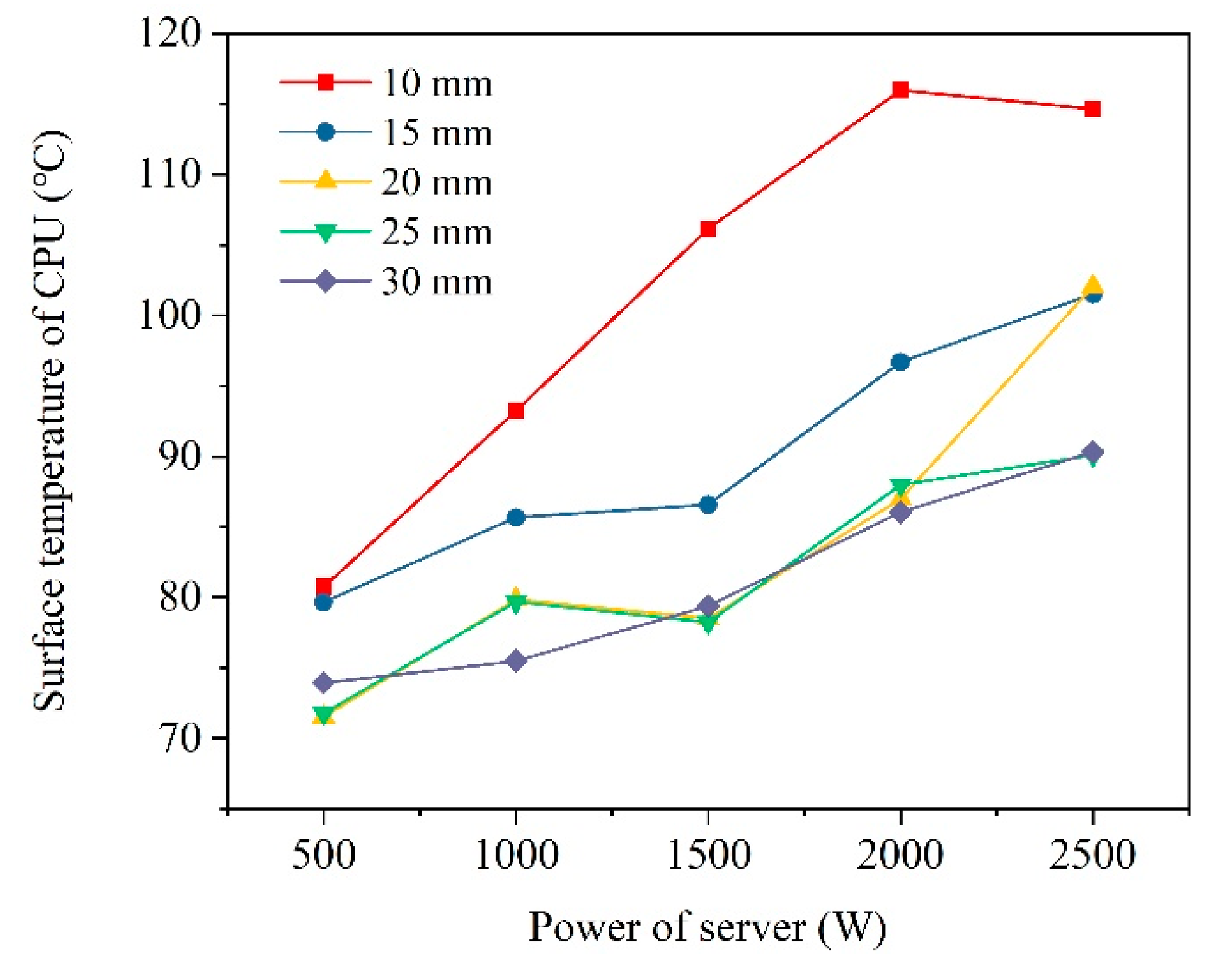
• For a given fluid-containing tank, a closer interval between servers would cause a higher server surface temperature. CFD simulations demonstrated the predicted surface temperatures of the servers under various IT loads;
• To maintain the surface temperature of the servers below 85 °C, an interval of 15 mm was needed for the server power to reach 1000 W. For a power of 1500 W, the interval must at least 20 mm. For a power larger than 2000 W or 3000 W, even an interval of 30 mm was not sufficiently large to maintain the surface temperature below 85 °C.

The COP and PUE were dependent on the room temperature and the fan and pump speed of the external heat exchanger. It would be interesting to study these influence factors, and this could allow for a more transparent interpretation of the results in future studies.

References

1. Król, A. The Application of the Artificial Intelligence Methods for Planning of the Development of the Transportation Network. Transp. Res. Procedia 2016, 14, 4532–4541. [Google Scholar] [CrossRef] [Green Version]
2. Bae, J.S.; Yong, S.C.; Kim, J.S.; Min, Y.C. Architecture and performance evaluation of MmWave based 5G mobile communication system. In Proceedings of the 2014 International Conference on Information & Communication Technology Convergence, Busan, Korea, 22–24 October 2014. [Google Scholar]
3. Fei, F.; Qi, Q.; Liu, A.; Kusiak, A. Data-driven smart manufacturing. J. Manuf. Syst. 2018, 48, 157–169. [Google Scholar]
4. Amisha, P.M.; Pathania, M.; Rathaur, V.K. Overview of artificial intelligence in medicine. J. Fam. Med. Prim. Care 2019, 8, 2328. [Google Scholar] [CrossRef]
5. Yong-Bin, Y.A.N.G. The Application Research of Data Mining Technique in Education. Comput. Sci. 2006, 33, 284–286. [Google Scholar]
6. Meng, X.; Zhou, J.; Zhang, X.; Luo, Z.; Gong, H.; Gan, T. Optimization of the thermal environment of a small-scale data center in China. Energy 2020, 196, 117080. [Google Scholar] [CrossRef]
7. Weissberger, A. Synergy Research Group: Hyperscale Data Center Count > 500 as of 3Q-2019. Available online: https://techblog.comsoc.org/2019/10/19/synergy-research-group-hyperscale-data-center-count-500-as-of-3q-2019/ (accessed on 19 October 2019).
8. Andrae, A.S.G. Total Consumer Power Consumption Forecast. Available online: https://10times.com/nordic-digital-business-summit (accessed on 1 October 2017).
9. Davies, G.F.; Maidment, G.G.; Tozer, R.M. Using data centres for combined heating and cooling: An investigation for London. Appl. Therm. Eng. 2016, 94, 296–304. [Google Scholar] [CrossRef]
10. Greenpeace, Potential Analysis on Energy Consumption of Data Centers and Renewable Energy in China 2019. Available online: https://www.greenpeace.org.cn/china-data-center-electricity-consumption-and-renewable-energy/ (accessed on 9 September 2019).
11. Jin, C.; Bai, X.; Yang, C.; Mao, W.; Xu, X. A review of power consumption models of servers in data centers. Appl. Energy 2020, 265, 114806. [Google Scholar] [CrossRef]
12. Chu, W.-X.; Wang, C.-C. A review on airflow management in data centers. Appl. Energy 2019, 240, 84–119. [Google Scholar] [CrossRef]
13. ASHRAE. Thermal Guidelines for Data Processing Environments; ASHRAE: Atlanta, GA, USA, 2015. [Google Scholar]
14. ASHRAE. PUE: A Comprehensive Examination of the Metric; ASHRAE: Atlanta, GA, USA, 2012. [Google Scholar]
15. Beghi, A.; Cecchinato, L.; Mana, G.D.; Lionello, M.; Rampazzo, M.; Sisti, E. Modelling and control of a free cooling system for Data Centers. Energy Procedia 2017, 140, 447–457. [Google Scholar] [CrossRef]
16. Ko, J.-S.; Huh, J.-H.; Kim, J.-C. Improvement of Energy Efficiency and Control Performance of Cooling System Fan Applied to Industry 4.0 Data Center. Electronics 2019, 8, 582. [Google Scholar] [CrossRef] [Green Version]
17. Khalaj, A.H.; Halgamuge, S.K. A Review on efficient thermal management of air- and liquid-cooled data centers: From chip to the cooling system. Appl. Energy 2017, 205, 1165–1188. [Google Scholar] [CrossRef]
18. Daraghmeh, H.M.; Wang, C.-C. A review of current status of free cooling in datacenters. Appl. Therm. Eng. 2017, 114, 1224–1239. [Google Scholar] [CrossRef]
19. Weerts, B.A.; Gallaher, D.; Weaver, R. Green Data Center Cooling: Achieving 90% Reduction: Airside Economization and Unique Indirect Evaporative Cooling. In Proceedings of the 2012 IEEE Green Technologies Conference, Tulsa, OK, USA, 19–20 April 2012. [Google Scholar]
20. Niemann, J.; Avelar, V. Economizer Modes of Data Center Cooling Systems; White Paper; Schneider Electric: Rueil-Malmaison, France, 2013; p. 132. [Google Scholar]
21. Schmidt, R.R.; Cruz, E.E.; Iyengar, M. Challenges of data center thermal management. IBM J. Res. Dev. 2005, 49, 709–723. [Google Scholar] [CrossRef]
22. Patankar, S.V. Airflow and cooling in a data center. J. Heat Transf. 2010, 132, 073001. [Google Scholar] [CrossRef]
23. Tuma, P.E. The merits of open bath immersion cooling of datacom equipment. In Proceedings of the 2010 26th Annual IEEE Semiconductor Thermal Measurement and Management Symposium (SEMI-THERM), Santa Clara, CA, USA, 21–25 February 2010. [Google Scholar]
24. Qiu, L.; Dubey, S.; Choo, F.H.; Duan, F. Recent developments of jet impingement nucleate boiling. Int. J. Heat Mass Transf. 2015, 89, 42–58. [Google Scholar] [CrossRef]
25. Robinson, A.J.; Colenbrander, J.; Byrne, G.; Burke, P.; McEvoy, J.; Kempers, R. Passive two-phase cooling of air circuit breakers in data center power distribution systems. Int. J. Electr. Power Energy Syst. 2020, 121, 106138. [Google Scholar] [CrossRef]
26. Deymi-Dashtebayaz, M.; Valipour-Namanlo, S. Thermoeconomic and environmental feasibility of waste heat recovery of a data center using air source heat pump. J. Clean Prod. 2019, 219, 117–126. [Google Scholar] [CrossRef]
27. Chen, H.; Cheng, W.-L.; Zhang, W.-W.; Peng, Y.-H.; Jiang, L.-J. Energy saving evaluation of a novel energy system based on spray cooling for supercomputer center. Energy 2017, 141, 304–315. [Google Scholar] [CrossRef]
28. Cho, J.; Kim, Y. Improving energy efficiency of dedicated cooling system and its contribution towards meeting an energy-optimized data center. Appl. Energy 2016, 165, 967–982. [Google Scholar] [CrossRef]
29. Dong, K.; Li, P.; Huang, Z.; Su, L.; Sun, Q.J.P.E. Research on Free Cooling of Data Centers by Using Indirect Cooling of Open Cooling Tower. Procedia Eng. 2017, 205, 2831–2838. [Google Scholar] [CrossRef]
30. Lu, T.; Lü, X.; Remes, M.; Viljanen, M. Investigation of air management and energy performance in a data center in Finland: Case study. Energy Build. 2011, 43, 3360–3372. [Google Scholar] [CrossRef]
31. Wu, C.; Tong, W.; Kanbur, B.B.; Duan, F. Full-scale Two-phase Liquid Immersion Cooing Data Center System in Tropical Environment. In Proceedings of the 2019 18th IEEE Intersociety Conference on Thermal and Thermomechanical Phenomena in Electronic Systems (ITherm), Las Vegas, NV, USA, 28–31 May 2019. [Google Scholar]
32. Kanbur, B.B.; Wu, C.; Fan, S.; Tong, W.; Duan, F. Two-phase liquid-immersion data center cooling system: Experimental performance and thermoeconomic analysis. Int. J. Refrig. 2020, 118, 290–301. [Google Scholar] [CrossRef]
33. Choi, E.J.; Park, J.Y.; Kim, M.S. Two-phase cooling using HFE-7100 for polymer electrolyte membrane fuel cell application. Appl. Therm. Eng. 2019, 148, 868–877. [Google Scholar] [CrossRef]
34. Ahmadi, V.E.; Erden, H.S. A parametric CFD study of computer room air handling bypass in air-cooled data centers. Appl. Therm. Eng. 2020, 166, 114685. [Google Scholar] [CrossRef]
35. Hassan, N.M.S.; Khan, M.M.K.; Rasul, M.G. Temperature Monitoring and CFD Analysis of Data Centre. Procedia Eng. 2013, 56, 551–559. [Google Scholar] [CrossRef]
36. Fulpagare, Y.; Bhargav, A.; Joshi, Y. Dynamic thermal characterization of raised floor plenum data centers: Experiments and CFD. J. Build. Eng. 2019, 25, 100783. [Google Scholar] [CrossRef]
37. Nada, S.A.; Said, M.A.; Rady, M.A. CFD investigations of data centers’ thermal performance for different configurations of CRACs units and aisles separation. Alex. Eng. J. 2016, 55, 959–971. [Google Scholar] [CrossRef]
38. Cheng, C.-C.; Chang, P.-C.; Li, H.-C.; Hsu, F.-I. Design of a single-phase immersion cooling system through experimental and numerical analysis. Int. J. Heat Mass Transf. 2020, 160, 120203. [Google Scholar] [CrossRef]
39. Ali, A. Thermal performance and stress analysis of heat spreaders for immersion cooling applications. Appl. Therm. Eng. 2020, 181, 115984. [Google Scholar] [CrossRef]
40. An, X.; Arora, M.; Huang, W.; Brantley, W.C.; Greathouse, J.L. 3D Numerical Analysis of Two-Phase Immersion Cooling for Electronic Components. In Proceedings of the 2018 17th IEEE Intersociety Conference on Thermal and Thermomechanical Phenomena in Electronic Systems (ITherm), San Diego, CA, USA, 29 May–1 June 2018; pp. 609–614. [Google Scholar]
41. NovecTM 7100 Engineered Fluid; 3MTM Ltd.: Saint Paul, MN, USA, 2020.
42. Valizadeh, K.; Farahbakhsh, S.; Bateni, A.; Zargarian, A.; Davarpanah, A.; Alizadeh, A.; Zarei, M. A parametric study to simulate the non-Newtonian turbulent flow in spiral tubes. Energy Sci. Eng. 2020, 8, 134–149. [Google Scholar] [CrossRef] [Green Version]
43. de Schepper, S.C.K.; Heynderickx, G.J.; Marin, G.B. Modeling the evaporation of a hydrocarbon feedstock in the convection section of a steam cracker. Comput. Chem. Eng. 2009, 33, 122–132. [Google Scholar] [CrossRef]
44. Malalasekera, W.; Versteeg, H. An Introduction to Computational Fluid Dynamics; Pearson Prentice Hall: Madrid, Spain, 2007. [Google Scholar]
45. Knudsen, M.; Partington, J.R. The Kinetic. Theoryof Gases. Some Modern Aspects. J. Phys. Chem. 1935, 39, 307. [Google Scholar] [CrossRef]
46. Liu, Z.W.; Lin, W.W.; Lee, D.J.; Peng, X.F. Pool Boiling of FC-72 and HFE-7100. J. Heat Transf. 1999, 123, 399–400. [Google Scholar] [CrossRef]
47. Kamoshida, J.; Hirata, Y.; Isshiki, N.; Katayama, K.; Sato, K. Thermodynamic Analysis of Resorption Heat Pump Cycle Using Water-Multicomponent Salt Mixture. In Heat Pumps; Pergamon: Oxford, UK, 1990. [Google Scholar]
48. ISO/IEC. 30134-2:2016 Information Technology—Data Centres—Key Performance Indicators—Part 2: Power Usage Effectiveness (PUE); ISO/IEC: Geneva, Switzerland, 2016. [Google Scholar]
49. Gupta, R.; Asgari, S.; Moazamigoodarzi, H.; Pal, S.; Puri, I.K. Cooling architecture selection for air-cooled Data Centers by minimizing exergy destruction. Energy 2020, 201, 117625. [Google Scholar] [CrossRef]
50. Silva-Llanca, L.; Ortega, A.; Fouladi, K.; del Valle, M.; Sundaralingam, V. Determining wasted energy in the airside of a perimeter-cooled data center via direct computation of the Exergy Destruction. Appl. Energy 2018, 213, 235–246. [Google Scholar] [CrossRef]
51. Esfandi, S.; Baloochzadeh, S.; Asayesh, M.; Ehyaei, M.A.; Ahmadi, A.; Rabanian, A.A.; Das, B.; Costa, V.A.F.; Davarpanah, A. Energy, Exergy, Economic, and Exergoenvironmental Analyses of a Novel Hybrid System to Produce Electricity, Cooling, and Syngas. Energies 2020, 13, 6453. [Google Scholar] [CrossRef]
52. Díaz, A.J.; Cáceres, R.; Cardemil, J.M.; Silva-Llanca, L. Energy and exergy assessment in a perimeter cooled data center: The value of second law efficiency. Appl. Therm. Eng. 2017, 124, 820–830. [Google Scholar] [CrossRef]
53. Ebrahimi, K.; Jones, G.F.; Fleischer, A.S. A review of data center cooling technology, operating conditions and the corresponding low-grade waste heat recovery opportunities. Renew. Sustain. Energy Rev. 2014, 31, 622–638. [Google Scholar] [CrossRef]
54. Nadjahi, C.; Louahlia, H.; Lemasson, S. A review of thermal management and innovative cooling strategies for data center. Sustain. Comput. Inform. Syst. 2018, 19, 14–28. [Google Scholar] [CrossRef]
Figure 1. Scheme of the proposed cooling system.
Energies 14 01395 g001
Figure 2. Two-phase cooling tank: (a) the tank, (b) servers, (c) condenser coil, and (d) primary heat exchanger.
Energies 14 01395 g002
Figure 3. Models for the tank and servers. (a) Mesh of the model (b) Grid section.
Energies 14 01395 g003
Figure 4. Correlation between liquid dynamic viscosity and temperature.
Energies 14 01395 g004
Figure 5. Correlation between vapor conductive coefficient and temperature.
Energies 14 01395 g005
Figure 6. Coefficient of performance (COP) and partial power usage effectiveness (pPUE) of the proposed two-phase cooling system.
Energies 14 01395 g006
Figure 7. The exergy efficiency of the proposed two-phase cooling system.
Energies 14 01395 g007
Figure 8. (a) Thermal map and (b) temperature distribution of the CPU server wallboard.
Energies 14 01395 g008
Figure 9. Schematic view of the heat transfer behavior during the boiling process.
Energies 14 01395 g009
Figure 10. Predicted surface temperatures of servers under different combinations: (a) 10 mm, (b) 15 mm, (c) 20 mm, (d) 25 mm, and (e) 30 mm.
Energies 14 01395 g010
Figure 11. Correlation between the server’s power and the average CPU temperature.
Energies 14 01395 g011
Figure 12. Differences in server surface temperature between intervals of 10 mm and 30 mm.
Energies 14 01395 g012