Abstract
Novel drivetrain concepts such as electric direct drives can improve vehicle dynamic control due to faster, more accurate, and more flexible generation of wheel individual propulsion and braking torques. Exact and robust estimation of vehicle state of motion in the presence of unknown disturbances, such as changes in road conditions, is crucial for realization of such control systems. This article shows the design, tuning, implementation, and test of a state estimator with individual tire model adaption for direct drive electric vehicles. The vehicle dynamics are modeled using a double-track model with an adaptive tire model. State-of-the-art sensors, an inertial measurement unit, steering angle, wheel speed, and motor current sensors are used as measurements. Due to the nonlinearity of the vehicle model, an Unscented Kalman Filter (UKF) is used for simultaneous state and parameter estimation. To simplify the difficult task of UKF tuning, an optimization-based method using real-vehicle data is utilized. The UKF is implemented on an electronic control unit and tested with real-vehicle data in a hardware-in-the-loop simulation. High precision even in severe driving maneuvers under various road conditions is achieved. Nonlinear state and parameter estimation for all wheel drive electric vehicles using UKF and optimization-based tuning is shown to provide high precision with minimal manual tuning effort.
1. Introduction
For realization of vehicle dynamic control and driver assistance systems, knowledge of the dynamic state variables of the vehicle motion is necessary. As the tires are the only connection to the road, transmitted tire forces and the tire slip, which is a variable for each tire derived from vehicle motion, are also important quantities to be determined. Next, to direct measurement by sensors, state estimators are used to determine the vehicle’s dynamic states and tire forces. This is done, on the one hand, because not all the required variables can be measured directly and, on the other hand, in order to save costs by eliminating the need for certain sensors. Recent literature reviews have shown that there are two main methods for state estimation: observer-based and neural-network-based or data-driven methods [1,2]. Observer-based approaches, which utilize different kinds of vehicle models, are the most common. While these methods can offer highly accurate results, the computational complexity can be a problem in practical real-time applications. Neural network-based approaches are used to overcome the need of a vehicle model and to be suitable for a real-time environment, since computational effort is reduced. The low robustness of these approaches regarding environmental or vehicle physical changes, for example in road conditions, are a major drawback [1]. Therefore, in the following, neural-network-based approaches are not considered further. For vehicle state estimation, two important questions are identified in [2], extending the range of estimation towards connected and automated driving vehicles and overcoming challenges due to nonlinear system behavior. The latter will be addressed in this article.
In the observer-based state estimator, a mathematical-physical model of the driving behavior, which can be kinematic, dynamic, or a combination of both, is used. If the model parameters are time-varying or uncertain, a combined state and parameter estimation can be performed by using a suitable approach [3]. In the context of vehicle models, tire parameters often are uncertain due to changing road conditions or tire wear. As combined state and parameter estimation leads to a nonlinear problem, concepts such as the Extended Kalman Filter [3] (EKF) or the Unscented Kalman Filter [4] (UKF) are frequently used. With the same sampling time, the UKF is able to approximate nonlinearities better than the EKF while being easier to implement [4] and requiring comparable computational effort [5]. An approach for simultaneous vehicle state and tire model parameter estimation using the EKF is shown in [6]. The authors use a spatial double track model with unknown road inclination and slope as well as Magic Formula tire models with uncertain parameters and wheel-individual adaption. Measured variables are the vehicle accelerations and yaw rate, which are captured by an Inertial Measurement Unit (IMU) as well as speed and position from a Differential Global Positioning System (DGPS) receiver. Furthermore, steering angle, wheel speeds, and wheel load forces are measured as they are used as system inputs. As shown in [1], GPS-aided methods are frequently used together with observers to overcome estimation gaps or inaccuracies. However, low GPS sampling frequencies, impaired signal availability in densely built areas, and additional cost are reasons why GPS usually does not come into use in state estimation for vehicle dynamic control. Instead, IMUs, steering angle, and wheel speed sensors are the state-of-the-art in nearly every modern vehicle. In [7,8], UKFs with double-track vehicle and Magic Formula tire models as well as the mentioned standard sensors are used for state estimation. Both authors assume the maximum tire road friction coefficient to be time-varying while this parameter is furthermore assumed to be common to all four tire models. This has the advantage that information about this parameter can be obtained and used on all wheels. In contrast, situations where the maximum tire road friction coefficient at each wheel is different may result in worse estimation than with wheel-individual parameter estimation. In [9,10], it is shown that UKF-based vehicle state and wheel-individual tire parameter estimation can be performed using only standard sensors and torque measurements from electric wheel hub motors. Furthermore, it is shown that the use of vehicle speed measurement by the Global Positioning System (GPS) offers advantages in only a few situations. Other approaches for UKF-based vehicle state estimation are shown in [11,12], where the filters are adaptive with respect to the process or measurement noise. The performance of the approaches is proven during simulations of severe driving maneuvers.
The task of unscented Kalman Filter tuning can be conducted in an efficient way by using optimization-based methods for estimation error minimization. Using the example of vehicle dynamic state estimation, this is shown in [13]. In [14], the approach is successfully applied to the problem of battery state of charge estimation using an EKF, where the process model parameters are optimized in the first and the Kalman filter’s covariance matrices in the second step. This paper shows the design and validation of a UKF-based vehicle state estimator with wheel-individual tire model adaption. Estimator tuning is carried out by an offline minimization of estimation error for real-vehicle driving maneuvers with an all-wheel drive electric vehicle. Then, real-time capability of the approach is investigated.
2. Materials and Methods
In the following, the vehicle model, the used sensors, as well as a short overview of the UKF algorithm are presented. Then, the filter tuning method is explained in detail.
2.1. Vehicle Model
For online vehicle state estimation, a model is needed that is capable of correctly representing dynamic motion, even in severe driving maneuvers, and at the same time requires low computational effort. Such a model is the planar double-track model, which will be used in the following. For simplicity, the vertical motion of the wheels is neglected, which means that the wheel contact points are all located in a common road plane. Furthermore, it is assumed that the steering angle on both front wheels is the same and that the wheels are rigidly coupled to the vehicle chassis. The road slope and inclination are assumed to be zero, and the masses of all vehicle components are combined in a common vehicle mass. The transformation from wheel coordinates, denoted by index w, to vehicle coordinates is performed with steering angle and
Thus, tire forces in vehicle coordinates are
The indices , , , and denote the front left, front right, rear left, and rear right wheels. Longitudinal velocity , lateral velocity , and yaw rate dynamics are modeled according to the force and torque equilibrium:
with vehicle mass m, yaw inertia , air density , drag coefficient , vehicle frontal area A, and distances and from center of gravity (CG) to front and rear axle as well as front and rear track width and . Wheel load forces are important for longitudinal and lateral tire force calculation. To keep the system model order small, the stationary wheel load forces are used in the following according to
The height of above the center of the wheels is denoted as , while , , , and denote the front and rear suspension roll and pitch stiffness. As an electric vehicle with four individually driven wheels is considered in this paper, the torque balance at each wheel includes the motor torque and the braking torque and , the longitudinal tire force , and the rolling resistance force according to
The dynamic tire rolling radius is [15]. For tire slip calculation, first, the wheels translational velocities are determined:
Then, longitudinal and lateral tire slip and for each wheel as well as the resulting tire slip are calculated according to
with numerical speed , which is required to avoid division by zero during vehicle standstill [16]. Furthermore, the transient behavior of the vehicle model for low velocities can be adjusted with this parameter. In this paper, tire forces are represented with a Burckhardt model, which uses only three parameters to define the slip dependent tire friction curve [17]. Thus, the effort for model identification is reduced compared to more sophisticated models such as Magic formula [18]. However, the accuracy is reduced, which must be taken into account when developing the estimator. The division into longitudinal and lateral tire forces at each wheel is performed by means of the Kamm’s circle [17], which gives
To allow for changes in the tire model, the nominal resulting tire force is scaled by an unknown friction coefficient , which has to be estimated. Examples of typical curves of tire road friction coefficient over tire slip for different road surfaces and conditions are shown in Figure 1. For small tire slip, the curve increases linearly, followed by a maximum and a decrease in tire friction coefficient for large slip values, which leads to a reduction in transmitted tire forces. The gradient of the linear region is mainly determined by parameters and .
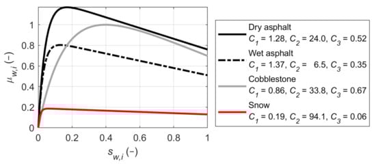
Figure 1.
Sample tire curves and corresponding model parameters for different road surfaces and conditions [19].
2.2. Sensors
In the context of vehicle stability control, several sensors have become state-of-the-art, so they can be found in nearly every vehicle. In this paper, these types of sensors are used. First, a low-cost MEMS-IMU (Microelectromechanical System) measures the vehicle’s longitudinal and lateral acceleration and as well as the yaw rate . Second, steering angle is calculated from the measured steering wheel angle and the steering ratio. Third, wheel speeds are measured by wheel speed encoders, and last, as the vehicle has an electric motor at each wheel, motor torques can be calculated from the measured motor currents. The relation between vehicle states and measured accelerations is approximately
The remaining measured variables are identical to the respective state or input variables. For the later design of the estimator, an optical reference speed sensor is used, which is mounted in the rear of the vehicle. Therefore, the measured speed is a superposition of translational speed and yaw rate according to
with and denoting the optical velocity sensors’ position relative to the center of gravity.
2.3. Unscented Kalman Filter
In the following, a short summary of the used UKF algorithm is given. A more detailed description can be found in [3,4,5]. It is assumed that there is a nonlinear time discrete system at time step k with additive system disturbance and output disturbance vectors according to
where denotes the state and the output vector. The disturbances are assumed to be Gaussian white noise with
where and are the corresponding covariance matrices. Furthermore, for simplification, it is assumed that and are uncorrelated. For the unscented transformation, a set of Sigma points with
is formed, where is the estimate of the state vector; is the state vector dimension; is the estimate of the state covariance; and is the jth row of the matrix square root, for example, calculated with the Cholesky decomposition [4]. In the a priori step, the Sigma points are transformed from time step to time step k with the state equation:
and the a priori estimate of the state vector and its covariance are computed according to
Then, a new set of Sigma points is calculated based on the a priori estimate and transformed with the output equation:
To reduce computational effort, the recalculation of the Sigma points can be omitted and the transformed Sigma points from the a priori step can be reused with the disadvantage of a possible loss of accuracy. After that, estimates of the output vector and its covariance are calculated together with the cross-covariance between state and output vector:
Finally, the a posteriori estimates of the state vector and its covariance can be calculated with
Tuning of the UKF is performed by choosing suitable values for the elements of and as well as the initial conditions and . In principle, there is a high number of degrees of freedom for the choice of the covariance matrices, why UKF tuning can be a challenging task. Several methods have been developed of which the optimization based method will be used in the next section for estimator design. Furthermore, the design of the tire model adaption is described and the used experimental vehicle is shown.
2.4. Estimator Design and Tuning
For tire model adaption to modeling errors as well as changing road conditions, is considered as a time-varying stochastic process. As this variable is assumed to be auto correlated, it is modeled with first-order dynamics according to
with the correlation time and an unknown disturbance , which is assumed to be Gaussian white noise [6]. To ensure that has physically plausible values, it is constrained by the Tangens hyperbolicus function. The state vector with unknown tire model adaption parameters is
The input and output vectors are
and the state space model according to Equation (12) is derived from Equations (3)–(10). Model parameters can be found in Table 1. For time discretization, the explicit Euler method [20] is used with a discrete sample time . As the tire forces in (9) depend on the wheel load forces (4), an algebraic loop results. To eliminate this algebraic loop, wheel load forces from the previous time step are used for tire force calculation, which results in

Table 1.
Model parameters.
For state estimation, observability of the system with the considered measurements is a fundamental requirement, which is examined here by linearizing the nonlinear system along a trajectory generated in numerical simulations. Then, the observability matrix of the linearized system is checked numerically [9]. The system is observable with the exception of vehicle standstill, where tire forces are close to zero and therefore is not observable. The sample times of the real sensors is . As can be seen, measurement sample times are significantly larger than for model discretization, why the estimator is implemented as a hybrid UKF [3]. This means, if no measurement is available, only a priori estimation is done. In accordance with Section 2.3, state and output disturbances and are assumed to be non-correlated additive vectors. For simplification, covariance matrices are chosen as time-invariant diagonal matrices with
and output vector dimension . As the output disturbances are mainly due to measurement noise, the elements of the measurement disturbance covariance matrix are chosen according to the noise properties given in the sensor data sheets (Table 2). If these are not available, the noise properties are approximately determined by evaluation of the sensor values when the system is in standstill. For a reduction in the degrees of freedom, it is assumed that the noise properties of the longitudinal and lateral accelerometers are identical. The same holds for the four wheel speed sensors. As the measured accelerations are not directly related to the states but are calculated with a model equation, an additional disturbance term is introduced, which results in
Table 2.
Sensor noise properties.
The structure of the state disturbance covariance matrix is chosen similarly:
For simplification, it is a valid assumption that the vehicle is in standstill at time step with high certainty and the initial estimation error covariance matrix can be chosen manually. Only the initial road friction coefficient adaption parameters are uncertain, while the corresponding values in are chosen bigger. Thus, the initial state estimate is
Determination of the elements of and is done in the following by optimization, where the problem
with the cost function in (31) solved first with the heuristic simulated annealing method [21] to reduce the probability of getting stuck in a local minimum. Afterwards, the accuracy of the result was increased with a constrained local optimization based on the Quasi-Newton method [21]. In both cases, Matlab’s implementation was used and the constraints were chosen as . For optimization, measurements from several driving maneuvers, which are carried out with an experimental electric vehicle with four wheel hub motors on different road surfaces (Figure 2), were used as training data. The cost function is the sum of squared errors between measured and estimated velocity , accelerations , and wheel speeds for all driving maneuvers j and time steps k. The errors were weighted by the matrix , and the cost for each driving maneuver j was normalized by the number of time samples . As the accelerations and wheel speeds were measurements of the UKF, there was a risk that was chosen to be very large as a result of the optimization in order to minimize estimation errors for these quantities. This could lead to large noise on the state and parameter estimates, which must be prevented by a suitable choice of the weighting matrix .
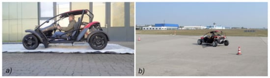
Figure 2.
Experimental electric vehicle BugEE with four wheel hub motors on (a) a wet road surface and (b) a dry road surface. Maximum torque for each front motor is ; maximum torque for each rear motor is ).
The intial solution for the optimization is chosen as
For optimization, the data from various driving tests were used, where excitation of longitudinal and lateral dynamics up to the limits of driving stability was carried out. Precise state and parameter estimation during these driving situations was required for the realization of vehicle dynamics control systems. The training data for optimization was taken from measurements captured during
- a transient slalom maneuver on wet road surface with , an initial velocity of , and a distance of between the obstacles, where high lateral tire slip occurs;
- a transient all-wheel-drive acceleration maneuver from standstill on wet road surface with with excessive longitudinal tire slip; and
- steady-state circular driving on dry road surface with and a constant radius from standstill to a velocity of , where the vehicle starts to oversteer.
To reduce the probability of overfitting during optimization, a wide range of different maneuvers has to be achieved. Since there are limitations in the available space on the test site, this requirement can only be met partially. The maneuvers are performed individually and the cost for all training data is added up. Details on the training data can be found in Appendix A. The result of the optimization is
Validation and discussion is carried out in the following section.
3. Results and Discussion
In this section, the state and parameter estimation for a set of test data containing four different driving maneuvers is examined. Details on the the complete data can be found in Appendix B, including estimated state variables, input and output variables, tire slip, and estimated tire curves. The reference values mean the measured values of the vehicle sensors and the optical speed sensor, while the reference tire slip values are computed from these. The maximum tire road friction coefficient is not measured but assessed from literature [19]. For generation of the validation results, the state and parameter estimator were implemented on a RCP-ECU (Rapid Control Prototyping-Electronic Control Unit) dSPACE MicroAutoBox II, which was connected to the vehicle sensors via CAN-Bus and operated with a sample time of . Sensor data were captured and saved during real world driving tests. For validation, this data can be replayed by a residual bus simulation. Thus, the real-time capability of online estimation with the shown approach for all four driving maneuvers can be examined by measuring the mean computing time . According to Table 3, the state estimator can be executed in real-time on the used ECU.
Table 3.
Mean computing time on RCP-ECU (Rapid Control Prototyping-Electronic Control Unit) for test data.
3.1. Wet Road Surface
In the following, the results from real world driving on wet road surfaces with low friction are presented. Artificial driving manuevers, more specifically, an all-wheel-drive acceleration from standstill and an emergency evasion was carried out.
3.1.1. Acceleration Maneuver
First, the results for an all-wheel-drive acceleration maneuver from standstill on a wet road surface (), similar to the maneuver used for training, are shown. Such a scenario could occur, for example, when starting on a slope in icy conditions, which is difficult to handle for average drivers. A traction control system might be necessary to support the driver in this situation, and therefore, precise estimates are needed. Maximum motor torque is applied to the wheels at and the vehicle starts to accelerate, which can be seen in Figure 3. After , wheel speeds using the left front and rear wheels as an example increase rapidly. The front wheel speed increase is smaller than at the rear wheels due to the larger maximum rear motor torque. Simultaneously, vehicle lateral velocity increases slowly due to a slight road bank angle. At , motor torque is quickly reduced to zero, which leads to a short period of vehicle yaw motion. After that, the vehicle rolls and lateral velocity as well as yaw rate converge to zero. High precision for longitudinal velocity estimation during the whole driving maneuver can be observed. The lateral velocity estimation shows some deviations, but these are bounded around the value measured with optical sensor. A reason for this might be the used tire model, which does not take different tire properties for longitudinal and lateral forces into account. Errors resulting from this simplification seem not to be compensated completely by the tire model adaption. As can be expected, yaw rate estimation is very accurate because this quantity is measured by a sensor.
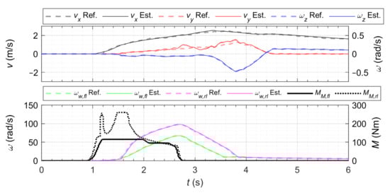
Figure 3.
Test data—acceleration on a wet road surface: measured and estimated velocities, yaw rate, wheel speeds, and motor torques for front left and rear left wheels.
The excessive longitudinal tire slip during the maneuver can be seen in Figure 4 using the left front and rear wheels as an example again. After a rapid increase at , the values stay at a high level for several seconds, which is estimated accurate. From , a small delay compared to the reference values is noticeable while the tire model adaption converges to a value of at the front and rear wheels. This value should correspond to the real maximum friction coefficient of the wet road surface. From to , the tire model adaption parameter is at a value of ≈1.7. As the tire slip stays in the linear region of tire curve at that time, this value does not represent the maximum friction coefficient. Instead, it indicates that the shape of with the used Burckhardt nominal tire model does not match the real road conditions exactly. An adjustment of parameters and might reduce the error or a more precise tire model could be used. Before and after , the adaption parameter is approximately 1, which means that the nominal tire model is used. In accordance with the errors that can be seen for lateral velocity estimation, some bounded lateral tire slip estimation errors occur. The shown scenario is very challenging for state and parameter estimation as high tire slip at all wheels occurs combined with lateral and yaw motion. Tire model uncertainties are maximal at this operating point, which is why therefore tire slip and adapted tire road friction coefficient must be estimated simultaneously. Under normal circumstances, low tire slip for at least one wheel aids velocity and thus tire slip estimation at the other wheels, but this is not the case here. Therefore, the results are considered very satisfactory.
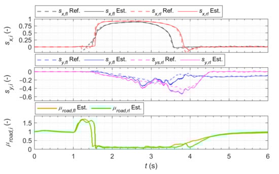
Figure 4.
Test data—acceleration on a wet road surface: measured and estimated tire slip for front left and rear left wheels as well as estimated tire model adaption parameter.
3.1.2. Emergency Evasion Maneuver
To validate the state and parameter estimation during a maneuver with large lateral tire slip, an emergency evasion maneuver on a wet road surface () is used as the test data. At the beginning of the maneuver, the longitudinal velocity is , as shown in Figure 5. A transient change in lateral acceleration and yaw rate is generated with a maximum lateral acceleration of . As the vehicle oversteers, it has to be stabilized by the driver. Due to the low friction surface, a considerable amplitude of lateral velocity occurs, which is estimated precisely. The errors in longitudinal velocity and yaw rate estimation are small.
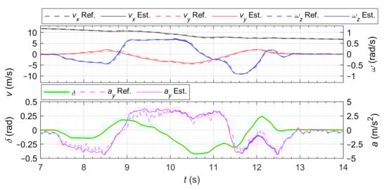
Figure 5.
Test data—evasion maneuver on a wet road surface: measured and estimated velocities, yaw rate, lateral acceleration, and steering angle.
Tire slip during the maneuver is shown for the front left and rear left wheels in Figure 6. Maximal lateral tire slip values are reached for both front and rear wheels at . With an amplitude of , the tire is clearly above the maximum of the tire curve. Nevertheless, estimation is very precise. In the moment of maximum lateral tire slip, the longitudinal tire slip at the front wheels also reaches a value of due to steering motion, which are also estimated accurately. This is again due to an adaption of the nominal tire model. The adaption parameter is estimated with from . As the tire mostly operates in the nonlinear region during this period of time, the value should represent the true maximum friction coefficient for the wet road surface. Deviations and fluctuations in the value result from different other disturbances, such as modeling errors, e.g., neglected tire force dynamics and suspension motion. In summary, the results for the evasion maneuver can also be considered satisfactory. This is important for yaw stabilization during emergency evasion of obstacles, which is a common use case for vehicle stability control.
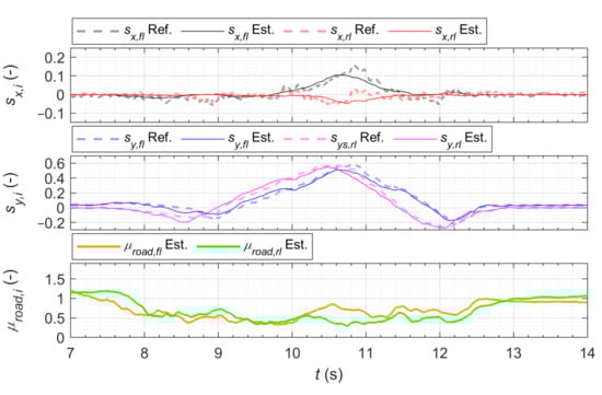
Figure 6.
Test data—evasion maneuver on a wet road surface: measured and estimated tire slip for front left and rear left wheels as well as estimated tire model adaption parameter.
3.2. Dry Road Surface
The maximum tire forces that can be transmitted on dry road surfaces are considerably higher than on wet road surfaces; therefore, the handling becomes unstable at significantly higher accelerations. Nevertheless, situations can occur where the driver loses control of the vehicle and stability control and, thus, precise state estimation is needed. In the following, a steady-state circle and a slalom driving maneuver are used for examination of the UKF performance.
3.2.1. Steady-State Circular Driving
The third driving maneuver is steady-state circular driving from standstill with low acceleration and a constant steering angle on a dry road surface (). By slowly increasing the velocity, the vehicle becomes unstable at the end of the maneuver and starts oversteering, why the driver has to stabilize the vehicle. As can be seen in Figure 7, a maximum lateral acceleration of is reached, which is in the typical range for road vehicles. The longitudinal and lateral velocity are estimated precisely during the phase of stable driving behavior from as well as during the phase of oversteering and stabilizing from . As before, yaw rate estimation is very precise due to the availability of measurement.
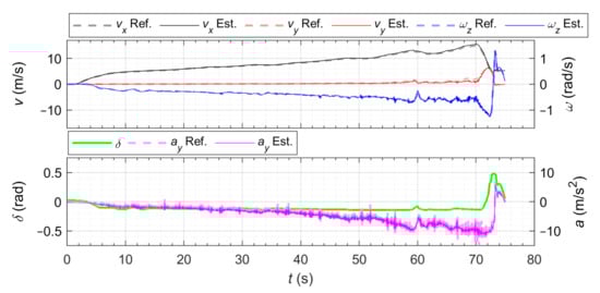
Figure 7.
Test data—circular steady-state driving maneuver on dry road surface: measured and estimated velocities, yaw rate, lateral acceleration, and steering angle.
Longitudinal and lateral tire slip are shown in Figure 8. The lateral tire slip at the front wheels is bigger than at the rear wheels until because of the steering angle. Both front and rear tire slip values decrease slightly during this period of time, while a rapid increase during oversteering can be observed. The lateral tire slip estimation is precise during the whole maneuver, but some bounded estimation errors occur during . In this time frame, the tire operates at the end of the linear region near the maximum of the tire curve, where the used Burckhardt nominal tire model is not very precise, as stated before. Longitudinal tire slip estimation shows some larger errors from , while the rapid increase in front wheel longitudinal tire slip is estimated precisely. The error might result from larger deviations in wheel radius, which occur because a different tire was mounted on the test vehicle than in the previously shown maneuvers. Nevertheless, the state and parameter estimator is robust against such model errors. The estimated tire model adaption parameter increases from a value of 1 up to until . As the tire is still in the linear region of the tire curve, this value does not represent the maximum tire road friction coefficient but the errors in the used tire curve. During oversteering at , when the tire operates near the maximum of the tire curve, can be seen as an estimate of with a plausible value of . Again, the states and parameters of the vehicle are estimated precisely during the critical driving situation with instable vehicle behavior.
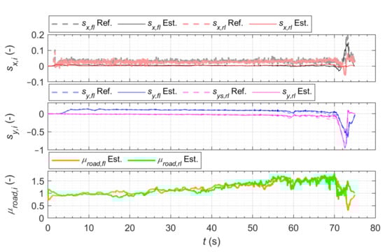
Figure 8.
Test data—circular steady-state driving maneuver on dry road surface: measured and estimated tire slip for the front left and rear left wheels as well as estimated tire model adaption parameter.
3.2.2. Slalom Maneuver
Lastly, the estimator was validated using data from a slalom maneuver on dry road surface () at a constant velocity of and with a maximum lateral acceleration of . The maximum tire force was not reached during this maneuver, so the tire operates completely in the linear region but the tire slip change is very dynamic. As can be seen in Figure 9 and Figure 10, precise estimation of the velocities and lateral tire slip is achieved. As during the circle driving maneuver, some bounded errors in longitudinal tire slip estimation can be noticed, which are likely to occur due to deviations in real wheel radius from the value used by the model.
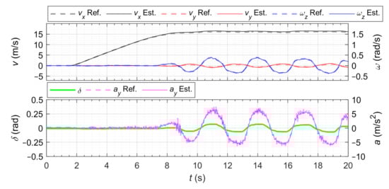
Figure 9.
Test data—Slalom maneuver on a dry road surface: measured and estimated velocities, yaw rate, lateral acceleration, and steering angle.
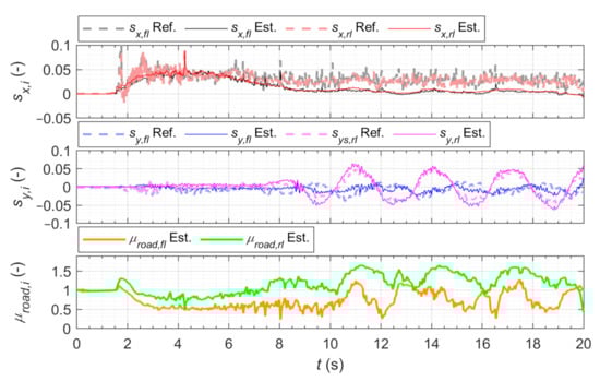
Figure 10.
Test data—Slalom maneuver on a dry road surface: measured and estimated tire slip for front left and rear left wheels as well as estimated tire model adaption parameter.
A wrong tire radius parameter directly influences the estimated tire forces and the resulting torques at the wheels. This error can be compensated up to a certain point by reduction of the longitudinal tire forces by the adaption parameter , as can be seen during the acceleration phase from . After this, lateral tire forces dominate and the adaption parameter mainly compensates errors in the nominal tire curve. As the longitudinal tire slip during this maneuver is below the level where a vehicle dynamics control system would operate, the shown errors are considered noncritical.
3.3. Estimated Tire Curves
The normalized tire forces over the resulting tire slip are shown in Figure 11 for each wheel and for all driving maneuvers. With respect to Equation (8), the displayed curves correspond to the adapted tire road friction coefficients . Even if the curves are corrupted by disturbances due to tire model errors, omitted tire force dynamics, and measurement noise, a branch for each road surface can be clearly identified. For dry roads, the curves for the steady-state circle and slalom maneuvers overlap. While the tire slip values stay in the linear region during the slalom maneuver, tire force saturation can be seen during the circle driving.
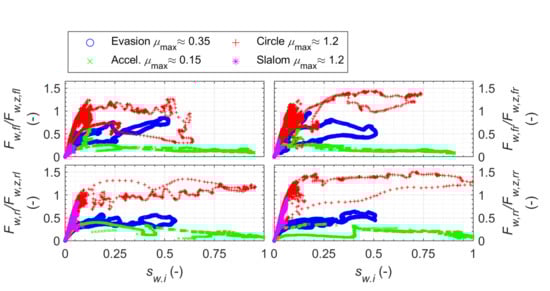
Figure 11.
Test data: estimated friction coefficient over tire slip for all driving maneuvers.
The estimated maximum friction coefficient on a dry road during circle driving surface is for the right and for the left wheels, which slightly differs from the expected values. A reason for this could be modeling errors in vertical tire force calculation, which become relevant during load change from inner curve to outer curve wheels. In addition, the errors in tire radius might contribute to discrepancies between the estimated and expected maximum friction coefficients. The estimated maximum friction coefficient for the evasion maneuver on a wet surface is , as expected. For each front wheel, a second branch with higher values for is visible, which is because the front wheels leave the wet surface area at the end of the maneuver and reach a dry road surface. During the acceleration maneuver, is estimated, which is in accordance with the values in the literature. The gradient is roughly identical for all considered ground surfaces.
4. Conclusions
The shown method estimates important dynamic states of the vehicle and adapts the tire model wheel-individually by means of a suitable modeling of the unknown disturbances with the help of the parameter . Even in severe driving situations, the suitability of the shown approach can be compared to reference measurements. By using a UKF, a nonlinear vehicle model can be used, while at the same time, a simple implementation is possible using a universal algorithm. The effort for the design of the UKF is low due to the use of optimization methods. Therefore, a high accuracy as well as a high robustness of the estimation against unknown disturbances, which exist in reality, are achieved by using training data from real driving tests, as has been shown during the validation. Furthermore, it has been shown that the state and parameter estimator can be executed on an ECU in real-time. The used Burckhardt tire model has few parameters and can be identified with small effort. By using a more precise tire model, it is assumed that a further increase in estimation accuracy can be achieved. For future developments, it should be examined how a model adaption regarding disturbances other than tire model variations, e.g., road slope and inclination, external wind, or deviations in tire radius, can be realized. A detailed analysis of the UKF estimation algorithm robustness to changes in the initial values of the states and parameters as well as the level of noise from the measurement data should be carried out in the future. Furthermore, it could be investigated how the accuracy and robustness of the estimation can be increased by using time-varying covariance matrices. Another issue is optimization of the UKF with respect to a correct estimation of , i.e., the estimation error covariance, which has not been considered. Closed-loop operation of the state estimator with a driving dynamic control system should also be investigated.
Author Contributions
Conceptualization, H.H. and M.S.; methodology, H.H.; software, H.H.; validation, H.H.; formal analysis, H.H.; investigation, H.H. and M.S.; resources, H.H. and M.S.; data curation, H.H.; writing—original draft preparation, H.H.; writing—review and editing, M.S.; visualization, H.H.; supervision, M.S.; project administration, M.S.; funding acquisition, M.S. All authors have read and agreed to the published version of the manuscript.
Funding
This research is part of the project “Competence Center eMobility” (ZS/2018/09/94461) funded by the European Regional Development Fund and the State of Saxony-Anhalt.
Institutional Review Board Statement
Not applicable.
Informed Consent Statement
Not applicable.
Data Availability Statement
The data presented in this study are openly available in OPEN SCIENCE Repository for Research Data and Publications of OvGU at 10.24352/UB.OVGU-2021-044.
Conflicts of Interest
The authors declare no conflict of interest.
Abbreviations
The following abbreviations are used in this manuscript:
| DGPS | Differential Global Positioning System |
| ECU | Electronic Control Unit |
| EKF | Extended Kalman Filter |
| GPS | Global Positioning System |
| IMU | Inertial Measurement Unit |
| MEMS | Microelectromechanical System |
| RCP | Rapid Control Prototyping |
| UKF | Unscented Kalman Filter |
Appendix A

Figure A1.
Training data: system inputs steering angle and motor torques.
Figure A1.
Training data: system inputs steering angle and motor torques.


Figure A2.
Training data: measured and estimated accelerations, velocities, yaw rate, and wheel speeds.
Figure A2.
Training data: measured and estimated accelerations, velocities, yaw rate, and wheel speeds.

Appendix B

Figure A3.
Test data: measured and estimated accelerations, velocities, yaw rate, and wheel speeds.
Figure A3.
Test data: measured and estimated accelerations, velocities, yaw rate, and wheel speeds.


Figure A4.
Test data: system inputs steering angle and motor torques.
Figure A4.
Test data: system inputs steering angle and motor torques.


Figure A5.
Test data: measured and estimated longitudinal tire slip.
Figure A5.
Test data: measured and estimated longitudinal tire slip.


Figure A6.
Test data: measured and estimated lateral tire slip.
Figure A6.
Test data: measured and estimated lateral tire slip.


Figure A7.
Test data: estimated unknown friction coefficients.
Figure A7.
Test data: estimated unknown friction coefficients.

References
- Chindamo, D.; Lenzo, B.; Gadola, M. On the Vehicle Sideslip Angle Estimation: A Literature Review of Methods, Models, and Innovations. Appl. Sci. 2018, 8, 355. [Google Scholar] [CrossRef]
- Jin, X.; Yin, G.; Chen, N. Advanced Estimation Techniques for Vehicle System Dynamic State: A Survey. Sensors 2019, 19, 4289. [Google Scholar] [CrossRef] [PubMed]
- Simon, D. Optimal State Estimation: Kalman, H [Infinity], and Nonlinear Approaches; Wiley-Interscience: Hoboken, NJ, USA, 2006. [Google Scholar]
- Julier, S.J.; Uhlmann, J.K. Unscented Filtering and Nonlinear Estimation. Proc. IEEE 2004, 92, 401–422. [Google Scholar] [CrossRef]
- van der Merwe, R. Sigma-Point Kalman Filters for Probabilistic Inference in Dynamic State-Space Models. Ph.D. Thesis, Oregon Health & Science University, Portland, OR, USA, 2004. [Google Scholar]
- Bechtloff, J.; Isermann, R. A redundant sensor system with driving dynamic models for automated driving. In Proceedings of the 15th Internationales Stuttgarter Symposium, Wiesbaden, Germany, 2 June 2015; Bargende, M., Reuss, H.C., Wiedemann, J., Eds.; Springer: Wiesbaden, Germany, 2015; pp. 755–774. [Google Scholar] [CrossRef]
- Antonov, S.; Fehn, A.; Kugi, A. Unscented Kalman filter for vehicle state estimation. Veh. Syst. Dyn. 2011, 49, 1497–1520. [Google Scholar] [CrossRef]
- Wielitzka, M.; Busch, A.; Dagen, M.; Ortmaier, T. Unscented Kalman Filter for State and Parameter Estimation in Vehicle Dynamics. In Kalman Filters—Theory for Advanced Applications; Ginalber Luiz de Oliveira Serra; InTech: London, UK, 2018; pp. 56–75. [Google Scholar]
- Heidfeld, H.; Schünemann, M.; Kasper, R. UKF-based State and tire slip estimation for a 4WD electric vehicle. Veh. Syst. Dyn. 2019, 58, 1479–1496. [Google Scholar] [CrossRef]
- Heidfeld, H.; Schünemann, M.; Kasper, R. Experimental Validation of a GPS-Aided Model-Based UKF Vehicle State Estimator. In Proceedings of the 2019 IEEE International Conference on Mechatronics (ICM), Ilmenau, Germany, 18–20 March 2019; pp. 537–543. [Google Scholar] [CrossRef]
- Luo, Z.; Fu, Z.; Xu, Q. An Adaptive Multi-Dimensional Vehicle Driving State Observer Based on Modified Sage-Husa UKF Algorithm. Sensors 2020, 20, 6889. [Google Scholar] [CrossRef] [PubMed]
- Wan, W.; Feng, J.; Song, B.; Li, X. Huber-Based Robust Unscented Kalman Filter Distributed Drive Electric Vehicle State Observation. Energies 2021, 14, 750. [Google Scholar] [CrossRef]
- Acosta, M.; Kanarachos, S. Optimized Vehicle Dynamics Virtual Sensing Using Metaheuristic Optimization and Unscented Kalman Filter. In Evolutionary and Deterministic Methods for Design Optimization and Control with Applications to Industrial and Societal Problems; Andrés-Pérez, E., González, L.M., Periaux, J., Gauger, N., Quagliarella, D., Giannakoglou, K., Eds.; Computational Methods in Applied Sciences; Springer International Publishing: Cham, Switzerland, 2019; Volume 49, pp. 275–290. [Google Scholar] [CrossRef]
- Bian, X.; Wei, Z.; He, J.; Yan, F.; Liu, L. A two-step parameter optimization method for low-order model-based state of charge estimation. IEEE Trans. Transp. Electrif. 2020, 1. [Google Scholar] [CrossRef]
- Schramm, D.; Hiller, M.; Bardini, R. Vehicle Dynamics: Modeling and Simulation, 2nd ed.; Springer: Berlin, Germany, 2018. [Google Scholar]
- Rill, G. Wheel Dynamics. In Proceedings of the XII International Symposium on Dynamic Problems of Mechanics (DINAME 2007), Ilhabela, Brazil, 26 February–2 March 2007. [Google Scholar]
- Burckhardt, M. Radschlupf-Regelsysteme: Reifenverhalten, Zeitabläufe, Messung des Drehzustands der Räder, Anti-Blockier-System (ABS), Theorie Hydraulikkreisläufe, Antriebs-Schlupf-Regelung (ASR), Theorie Hydraulikkreisläufe, elektronische Regeleinheiten, Leistungsgrenzen, ausgeführte Anti-Blockier-Systeme und Antriebs-Schlupf-Regelungen, 1st ed.; Vogel-Fachbuch: Würzburg, Germany, 1993. [Google Scholar]
- Pacejka, H.B. Tyre and Vehicle Dynamics, 2nd ed.; Elsevier/Butterworth-Heinemann: Amsterdam, The Netherlands, 2006. [Google Scholar]
- Tanelli, M.; Piroddi, L.; Piuri, M.; Savaresi, S.M. Real-time identification of tire-road friction conditions. In Proceedings of the 2008 IEEE International Conference on Control Applications, Antonio, TX, USA, 3–5 September 2008; IEEE Service Center: Piscataway, NJ, USA, 2008; pp. 25–30. [Google Scholar] [CrossRef]
- Lindfield, G.R.; Penny, J. Numerical Methods: Using MATLAB, 3rd ed.; Academic Press: Amsterdam, The Netherlands; Boston, MA, USA, 2012. [Google Scholar]
- Arora, R.K. Optimization: Algorithms and Applications; CRC Press Taylor & Francis Group: Boca Raton, FL, USA, 2015. [Google Scholar]


Publisher’s Note: MDPI stays neutral with regard to jurisdictional claims in published maps and institutional affiliations. |
© 2021 by the authors. Licensee MDPI, Basel, Switzerland. This article is an open access article distributed under the terms and conditions of the Creative Commons Attribution (CC BY) license (http://creativecommons.org/licenses/by/4.0/).