Abstract
The optimal siting and sizing of battery energy storage system (BESS) is proposed in this study to improve the performance of the seventh feeder at Nakhon Phanom substation, which is a distribution network with the connected photovoltaic (PV) in Thailand. The considered objective function aims to improve the distribution network performance by minimizing costs incurred in the distribution network within a day, comprising of voltage regulation cost, real power loss cost, and peak demand cost. Particle swarm optimization (PSO) is applied to solve the optimization problem. It is found that the optimal siting and sizing of the BESS installation could improve the performance of the distribution network in terms of cost minimization, voltage profile, real power loss, and peak demand. The results are investigated from three cases where case 1 is without PV and BESS installation, case 2 is with only PV installation, and case 3 is with PV and BESS installations. The comparison results show that case 3 provided the best costs, voltage deviation, real power loss, and peak demand compared to those of cases 1 and 2; system costs provided by cases 1, 2 and 3 are USD 4598, USD 5418, and USD 1467, respectively.
1. Introduction
Nowadays, the electricity demand has been increased due to the growth of population and the rapid improvement of various technologies resulting in the increase of electrical power generation to meet the demand. In the past decades, electrical power generation is mostly produced from fossil energy, which directly affects global warming from greenhouse gas emissions. For this reason, the electrical power generations generated from renewable energy sources (RESs) have received huge attention at present because they are clean energy sources that are not running out. However, the main limitation of the RESs is the fluctuation of the uncontrollable natural resources. At present, RESs have been widely connected to distribution networks, resulting in the unreliability and low power quality of the distribution networks from the uncertainty power generation. Especially, in Thailand, the investment of the RESs from companies has been increased according to the government’s encouragement, which directly affects the distribution network operators (DNO) because RESs are connected to the distribution networks. For this reason, energy storage systems (ESSs) have been used in the distribution networks with the connected RESs to deal with the uncertainty of the power generation problem from the RESs [1] and improve the performance of the distribution networks, especially voltage profile improvement and power loss reduction, which are the significant factors of power quality of DNO [2]. Moreover, the ESS in microgrid systems could be connected as a virtual central energy storage system when operating in interconnected multi-node microgrids [3].
Battery energy storage systems (BESSs) have been adopted for several objectives such as balancing load and improving voltage profile [4,5,6], minimizing total operation costs [7,8,9,10], minimizing power losses [11,12,13,14,15,16,17], peak shaving [18], improving the power system performance to support the increased load demand [19], and improving reliability and power quality of the power systems (multi-objective functions) [20,21,22,23,24,25,26,27,28,29]. Additionally, the optimal size of BESS installation to store electrical energy during the valley load period and supply it during the peak load period to maximize operational benefits was proposed in [30,31]. The BESS was installed in the wind farm for smoothing the power generation and reducing the operation costs [32,33,34,35], and in the microgrid with the connected photovoltaics (PV) to improve the reliability [36]. The BESS was also used as a voltage source or uninterruptible power supply of microgrid in case utility grid supply or RES is collapsed [37], and as a damping power oscillation in distribution networks [38]. Moreover, the optimal allocation of BESS was able to increase the profits from purchasing/selling the electrical energy [39,40,41] and set a fair price of electricity for both companies and customers [42].
Energy storage technologies can be categorized due to the physical characteristics, i.e., mechanical forms such as pumped hydro storage (PHS), compressed air energy storage (CAES), and flywheels; electromagnetic forms such as superconducting magnetic energy storage (SMES), and supercapacitors; and electrochemical forms such as batteries and hydrogen storage. However, the energy storage technologies, which can be applied to improve power quality, include flywheels, SMES, supercapacitors, and batteries. Among these, batteries are the only technology that can be used in short-term and long-term operations [43]. BESSs can be categorized according to types of batteries, such as the lead–acid battery, sodium-sulfur battery, redox flow battery, and lithium-ion battery (Li–ion) [44]. When comparing the characteristics of each battery technology, it is found that lead–acid battery is cheap (around 50–600 USD/kWh), but it has low energy density (20–30 Wh/kg) and less lifespan than other technologies. For sodium–sulfur battery, although it has a higher energy density (150–240 Wh/kg) than others, its operating temperature is very high (around 300 °C). Redox flow battery has a lower energy density (15–30 Wh/kg) than other technologies, which means that it requires more area and weight than other technologies at the same capacity. For Li–ion battery, even if it has a high energy density (90–190 Wh/kg) and long lifespan, the appropriate temperature control is required because the inappropriate temperature directly affects the lifespan of Li–ion battery [45]. In [46], the lead–acid and Li–ion batteries are tested in an off-grid system with the connected PV, and it is found that Li–ion battery has a double longer lifespan than lead–acid battery. It is also found that although the price of Li–ion battery is double of the lead–acid battery, Li–ion battery is more appropriate than lead–acid battery because the maintenance cost of Li–ion battery is lower due to its longer lifespan. Moreover, Li–ion battery has been widely used as the BESS in several applications especially in electric vehicles (EVs). This is because emission reduction from fuel vehicles is considered a very important task, and hence EVs and Li–ion batteries tend to be more popular [47]. Li–ion consists of various advantages, such as working in a wide range of voltage levels, high density of energy per volume, simple adjustable power and capacity, and long life cycles [48]. In addition, used Li–ion from EVs can be reused for other objectives, such as for energy balancing in thermal power plants, using it as an uninterrupted power supply (UPS), and using it as a BESS to reduce waste and highly utilize the battery [49]. More importantly, the cost of Li–ion battery has continuously decreased from 1160 USD/kWh in 2010 to 176 USD/kWh in 2018 [50], and it tends to drop to approximately 100 USD/kWh in 2023 [51]. Therefore, the Li–ion battery is adopted as the BESS in this study to improve the performance of the distribution network with the connected PV.
The BESS can be used at the maximize benefits with the considered objective function when it is installed at the optimal siting and sizing [12,14]. Thus, this study aims to improve the performance of the seventh feeder of Nakhon Phanom substation in Thailand, which is the distribution network with the connected PV by providing optimal siting and sizing of BESS installation where Li–ion is used as the BESS. The objective function is to improve the distribution network performance by minimizing the costs incurred in the distribution network within a day comprising of voltage regulation cost, real power loss cost, and peak demand cost. Fourier series is applied to define the state of energy (SoE) of the BESS, which indicates the amount of energy remaining in the battery in each period because Fourier series is the continuous signal that can express the SoE of the BESS for all considered period; this corresponds to the fact that the BESS power level in real-world applications is continuous. Moreover, the over-discharge must be efficiently prevented, which means charging quantity must be equal to discharging quantity in one cycle [24]. Particle swarm optimization (PSO) is adopted to find the minimum value of the objective function because its performance in obtaining the optimal siting and sizing of the BESS is verified in [52,53,54,55,56,57], and PSO has been also applied to efficiently solve several recent optimization problems in different fields [58,59,60]. The BESS installation simulation is conducted on the 56-bus realistic radial distribution network with the connected PV located at the seventh feeder of Nakhon Phanom substation, Thailand. The contribution of this research is to improve the performance of the realistic radial distribution network with the connected PV in terms of voltage profile improvement, power loss reduction, and peak demand reduction by providing optimal siting and sizing of the BESS installation. The dynamic load and PV data in each time period were really measured from the substation and PV installation point, respectively, which contains double the number of data than that used in [24,52]. Therefore, the results will be more accurate and be able to efficiently provide the optimal siting and sizing of the BESS in the real distribution networks with the connected PV.
2. BESS and Formulations
In this research, the Li–ion battery is chosen as the BESS to install in the realistic radial distribution network with the connected PV. The Fourier series is used in the BESS simulation to predict the SoE of the BESS.
2.1. BESS
The Li–ion has been widely used both in the literature and real-life applications because of its good qualities, such as fast charging, high energy-to-volume density, low self-discharge, and long-life service. However, Li–ion should not be used for a long period of operation because many factors, such as the number of battery operation cycles, depth of discharge (DoD), and temperature affect the lifetime of the Li–ion. Thus, for a long period of operation of Li–ion battery, a high-cycle operation should be avoided, DoD should not be over 80% of its maximum capacity, and the appropriate temperature is around 15–35 °C [61,62].
2.2. BESS Formulations
The BESS simulation in this research focuses on the charging and discharging rates by considering the energy difference of the BESS between the consecutive time interval of the SoE. The charging and discharging rates at each time interval in a one-day operation of the BESS (24 h) can be formulated as in Equation (1).
where is charging and discharging rates in the considered period, is the charging or discharging power of the BESS at times , and depends on the time interval that one-day operation hour is divided, such as considering every 1 h , 30 min , or 15 min , etc.
The Fourier series is applied to express the SoE of the BESS and its obtained by substituting the Fourier coefficient from Equation (2) into Equation (3).
where , , are the constant Fourier coefficient, Fourier cosine coefficients, and Fourier sine coefficients, respectively. is the number of Fourier coefficients, which is set to 8 for this study [24,52]. is the energy of the BESS at time . is the total time period (24 h).
The constant Fourier coefficient does not affect the determination of , but it is used to ensure that the SoE value is not less than zero or less than the minimum of DoD ().
To find the charging or discharging rate, which is the status, of the BESS at each time interval, the difference of energy levels of the BESS between the present period, , and the previous period, , is calculated as in Equation (4). If the value of is greater than or equal to zero, the BESS is in the state of charging, and if the value of is less than zero, the BESS is in the state of discharge. The charging and discharging rates can be found according to Equations (5) and (6), respectively [24].
where is the battery charging efficiency, is the battery discharging efficiency, is the total efficiency of the battery [24],, is the sampling time interval.
The optimal size of the BESS can be computed by Equation (7), and the lifespan of the BESS can be found from Equations (8) and (9) [24] as follows:
where is the optimal size of the BESS and the unit of the BESS depends on the unit of the battery energy value, and are the maximum and minimum energy of the BESS, is a maximum depth of discharge, which is set to 0.8 in this study [52], are the operation cycle of the BESS in a day, and are the magnitude energy of the BESS at time and − 1, respectively, is the total life cycles of the BESS, which is equal to 3221 cycles in this study [61], and is the period of the BESS operation (365 days).
3. Problem Formulations
The optimal siting and sizing of the BESS installation presented in this research is proposed to improve the performance of the distribution network with the connected PV in terms of voltage profile improvement, power loss reduction, and peak demand minimization. The technical constraints of the distribution network are also considered to ensure network security and limitations.
3.1. Objective Function
The objective function of the optimal siting and sizing of the BESS installation is to improve the distribution network performance by minimizing costs incurred in the distribution network caused by voltage deviation, real power loss, and peak demand, which are voltage regulation cost , real power loss cost , and peak demand cost, respectively. The calculation of these values can be found in the provided equations.
where is a total bus number, is the voltage per-unit of the bus at time , is the reference voltage (1 per-unit), is a voltage regulation cost rate (0.142 USD/p.u.) [23], is a total branch number, is an active power loss in each branch, is an active power loss cost rate (0.284 USD/kWh) [24], is a maximum peak demand of real power during the considered period, and is a peak demand cost rate (200 USD/kWh/year) [24].
This study aims to find the optimal siting and sizing of the BESS in the distribution network to improve the system performance in terms of voltage profile improvement, power loss reduction, and peak demand reduction. However, each term of improvement has different units; for example, voltage is in p.u., real power loss is in MW, and peak demand is in MW. Therefore, these terms are converted into costs incurred in the distribution network, caused by voltage deviation, real power loss, and peak demand, to calculate the objective function in the same aspect. Moreover, the battery costs such as cost to charge/discharge the battery, installation cost, and maintenance cost are excluded in the objective function. This is because if these battery costs are included in the objective function, the solutions will be obtained by partly considering minimum battery costs instead of fully considering system performance improvement. As a result, the truly appropriate siting and sizing of the BESS to improve the system performance in the stated terns will not be able to obtain.
3.2. Constraints
3.2.1. Voltage Constraint
Voltage magnitude at every bus for all considered time period must be in the standard range (±5% of ) as expressed in the given equation [52].
where are the lower and upper bounds of standard range voltage, respectively. is the voltage per-unit of the bus at time .
3.2.2. Line Constraint
The apparent power of each line is restricted in the power line limits as expressed in the following equation:
where is the apparent power flow from the ith bus to the jth bus, and is the maximum apparent power flow of the transmission line (p.f. = 1).
3.2.3. Battery Constraint
To ensure the BESS is operated within the power and capacity limits in all time intervals, the power and capacity of BESS are bounded by Equations (17) and (18), respectively.
where , are the minimum and maximum power of BESS, respectively, is a power charge of BESS at time , is a power discharge of BESS at time , and , and are the minimum and maximum energy of BESS, respectively.
4. Methodology
The optimal siting and sizing of the BESS installation in this study were operated on the distribution network with the connected PV. The results were simulated by using MATLAB with MATPOWER 7.0, N.Y., USA [63] interface. The PSO was adopted to evaluate the minimum value of the objective function for finding the optimal siting and sizing of the BESS installation.
4.1. Case Study
The distribution network used in this study is the seventh feeder of Nakhon Phanom substation, Thailand, which is a 56-bus distribution network as shown in Figure 1. The first bus is defined as the slack bus, and the detailed data of real and reactive powers at each bus and line impedance are provided in Table A1 in Appendix A, in which the base voltage is 12.66 kV, and the base power is 10 MVA. The PV (5.88 MW) was installed at the 47th bus and the output power of PV can be found in Table A2 in Appendix A. The load magnitudes of each bus at each time are defined according to Equations (19) and (20) for real power and reactive power, respectively. The PV power and load demand of the 56-bus distribution network are presented in Figure 2, in which these data are provided by Provincial Electricity Authority (PEA), Bangkok, Thailand. These PV power and load demand are chosen from the data collected over a year where the day when the reverse power flow reached the highest value was selected. Therefore, this study could improve the performance of the worst day and cover the problem of the other days.
where , are the real and reactive powers of the bus at time , respectively. , are the base real and reactive powers at the bus obtained from Table A1 in Appendix A, respectively. , are the real power coefficient and reactive power coefficient at time presented in Table A2 in Appendix A, respectively, to change the demand every considered time interval.
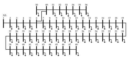
Figure 1.
Case study.
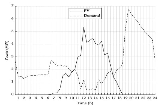
Figure 2.
Photovoltaic (PV) power and load demand.
4.2. PSO
The principle of PSO for solving optimization problems is inspired by the foraging behavior of a flock of birds or fishes [52]. The steps of the PSO process for solving problems are as follows: In the first step, the number of populations or particles () is defined where each particle consists of decision variables (), the starting position of each particle is initialized, and its velocity is initially set to zero. Afterward, the objective function is evaluated by using the initial positions and velocities of the particles, and then the initial personal best () of each particle and the initial global best () are obtained (the global best is the best particle among all personal bests). Following this, the inertia is calculated according to Equation (21). The velocity of each particle is then updated by Equation (22), and the position of each particle is also updated by Equation (23). The updated position of each particle is substituted to evaluate the objective function. Then, the personal best and global best are updated. Repeat the process until the maximum iteration is reached. The flowchart and pseudo-codes of PSO are shown in Figure 3 and Figure 4, respectively.
where is the velocity of the ith particle, is the personal best position of the ith particle, is the global best position, is the current position of the ith particle, is the inertia of , is a current iteration, is a maximum iteration, and are set to 2, and and are randomly generated numbers between 0 and 1.
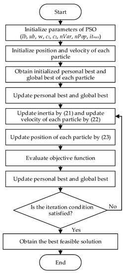
Figure 3.
Flowchart of particle swarm optimization (PSO).
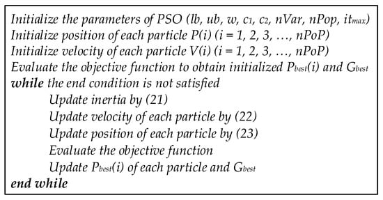
Figure 4.
Pseudo-codes of PSO.
4.3. The Procedure of the Optimal Siting and Sizing of the Battery Energy Storage System (BESS)
The procedure of the optimal siting and sizing of the battery energy storage system (BESS) can be described as the following steps:
- Model the distribution network as detailed in Section 4.1 in the MATPOWER;
- Define candidate buses in the distribution network;
- Choose one candidate bus to install the BESS;
- Solve the optimization problem by using PSO;
- Perform power flow calculation and evaluate the objective function;
- Repeat steps 4 and 5 if the maximum iteration is not reached; otherwise, proceed to step 7;
- Obtain the optimal Fourier coefficients of BESS installation at the considered bus from step 3;
- If the candidate bus is not the last candidate, return to step 3; otherwise, proceed to step 9;
- Obtain the optimal location and size of the BESS with the lowest objective function value;
- Substitute the Fourier coefficients provided from step 9 in Equations (1)–(9) to generate the parameters of the BESS.
The flowchart and pseudo-codes of the proposed method are shown in Figure 5 and Figure 6, respectively.
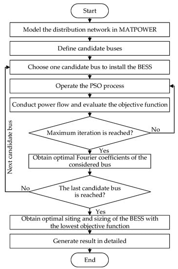
Figure 5.
Flowchart of the proposed method.
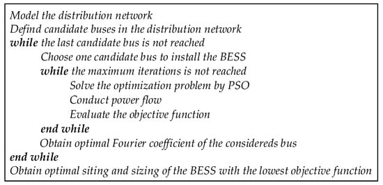
Figure 6.
Pseudo-codes of the proposed method.
4.4. System Performance Evaluation
The performance of the distribution network is evaluated in various terms by referring to the objective function, which comprises of voltage deviation index, power losses, and peak demand.
4.4.1. Voltage Deviation Index (VDI)
The voltage deviation index (VDI) is applied to evaluate the voltage profile improvement of the network. VDI is the maximum difference value between the voltage of each bus in the distribution network over 24 h and the reference voltage, presented in percent (). A smaller VDI value means a better voltage profile, and the VDI can be calculated by Equations (24) and (25).
where is the VDI of the ith bus, is the reference voltage (1 p.u.), is the voltage in p.u. of the ith bus, and is the total VDI of the distribution network.
4.4.2. Power Losses
The power losses incurred in the distribution network composed of real power loss, reactive power loss, and apparent power loss. These power losses can be computed by the provided equations.
where is the real power loss, is the reactive power loss, is the apparent power loss, is the real power loss of the lth branch, is the reactive power loss of the lth branch, is the total branch number. is a time interval, and is the total time period.
4.4.3. Peak Demand
The peak demand is considered from the real power flow at the slack bus over 24 h, in which the positive value of the real power flow indicates the power flowing into the network and the negative value of the real power flow indicates power flowing out of the network.
5. Results and Discussion
The optimal siting and sizing of the BESS installation are presented to improve the performance of the realistic distribution network with the connected PV, which is the seventh feeder of Nakhon Phanom substation in Thailand. The parameters of PSO were population number () = 60 and maximum iterations = 1000. The technical constraints of the distribution network consist of the voltage limits, which is ± 5% of the reference voltage (12.66 kV), and the rated line current, which is 410 A (the rated line current limit of the 185 sq.mm. Space aerial cable is according to the Provincial Electricity Authority (PEA) standard). The simulation is conducted in MATLAB interfaced with MATPOWER. The simulation results are compared between three cases where case 1 is without PV and BESS, case 2 is with only PV, and case 3 is with both PV and BESS.
5.1. Optimal Siting and Sizing of BESS Installation
The BESS is installed at each bus from the second to 56th bus to find the optimal location for the BESS installation. The values of the objective function of all three cases are shown in Table 1, in which case 3 shows the best five bus locations of the installed BESS, providing the minimum objective values together with the size and lifetime of the BESS. It is found that the best location for BESS installation to improve the distribution network performance is located at bus 47, which is the same location as PV installation, following by buses 46, 45, 44, and 43, respectively. Although the 48th bus is actually the bus that has the most voltage deviation problems, it is not a suitable bus for BESS installation to improve the network performance. It is also found from Table 1 that even though BESS installation at the 47th bus has the highest values of power and capacity, it is still the most appropriate location for the performance improvement due to the best value of the objective function (Csys). The lifetime values of BESS from each location are slightly different, but the 47th bus still has the longest lifetime, which is 8.71 years.

Table 1.
Optimal siting and sizing of BESS.
When comparing the costs incurred in the distribution network, including voltage regulation cost, real power loss cost, and peak demand cost, it is found that the costs from cases 1 and 2 are USD 4598 and USD 5418, respectively, and the costs from case 3 in which BESS is installed at the 47th bus is USD 1467. Hence, only PV installation could worsen the network performance. However, PV installation, together with the optimal siting and sizing of BESS installation, could efficiently improve the network performance.
The SoE of the BESS at the 47th bus over 24 h from 00:00 a.m. is presented in Figure 7 to observe when the BESS is charging or discharging, and charging/discharging rate can be obtained. It is noticeable that the energy of the BESS was slightly changed from 00:00 a.m to 6:00 a.m. and continuously decreased until reaching the lowest value, which is around 12.50 MWh, at 8:00 a.m. From 8:00 a.m. to 6:00 p.m. (at the 18th hour), the energy of the BESS was sharply increased until the maximum value, which is approximately 62.72 MWh. After that, the BESS was discharged from the maximum energy to its initial value at the last hour. It is found that the energy of the BESS was increased in the time when PV supplied energy to the network (6:30 a.m. to 6:00 p.m.) because BESS stored surplus energy from PV, which exceeded the demand in the network. Despite the discharge of some energy from 6:30 a.m. to 8:00 a.m., this was due to the network performance improvement by mainly considering the objective function. In the period when supply from PV was stopped, the SoE of BESS was also dropped to supply the stored energy back to the network. This could verify that the BESS could efficiently balance the supply and demand of the network.
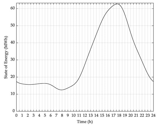
Figure 7.
The state of energy (SoE) of the BESS.
5.2. Voltage Deviations
The voltage deviations index () comparison of each case was obtained, as shown in Table 2. It can be derived that of case 3 is the lowest (146.46%), which means that the BESS installation could improve the voltage profile of the distribution network with the connected PV. In Figure 8, the voltage profile of the 48th bus where the voltage deviation problems are the most frequently detected in the distribution network over 24 h is presented. For cases 1 and 2, it was found that the voltage level was lower than the lower bound of the voltage limit from 6:30 p.m. (the 18th hour and a half) to 11:00 p.m. (the 23rd hour). In addition, for case 2, the voltage level was higher than the upper bound of the voltage limit from 11:30 a.m. (the 11th hour and a half) to 3:30 p.m. (the 15th hour and a half). For case 3, installing the BESS at the 47th bus could maintain the voltage level within the voltage limit range over 24 h.
Table 2.
System performance comparison.
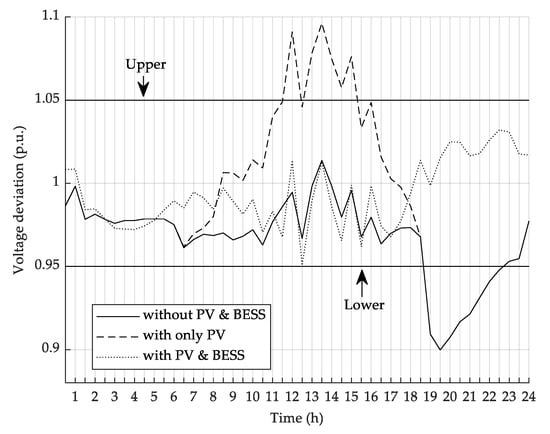
Figure 8.
Voltage profile of the 48th bus.
5.3. Power Losses
The real power losses of all three cases over 24 h are displayed in Figure 9. For case 1, the real power loss was continuously less than 0.05 MW from 00:00 a.m. to 6:30 p.m. (the 18th hour and a half), however, after that the real power loss of this case was considerably increased until reaching the maximum value at 7:30 p.m. (the 19th hour and a half), which is equal to 0.33 MW. For case 2, the real power loss has occurred the same as case 1 except for the period from 6:30 a.m. (the sixth hour and a half) to 6:30 p.m. (the 18th hour and a half). Especially, the loss for case 2 dramatically climbed to the highest point, which is 0.47 MWh at the 12th hour, and during the time from 10:30 a.m. (the 10th hour and a half) to 4:30 p.m. (the 16th hour and a half), the real power loss of this case was more than those of cases 1 and 3. For case 3, the real power loss was slightly more than those of cases 1 and 2 during 2:30 a.m. (the second hour and a half) to 5:00 a.m. (the fifth hour) and was slightly more than that of case 1 from 11:30 a.m. (the 11th hour and a half) to 3:30 p.m. (the 15th hour and a half). Moreover, the real power loss of case 3 was less than those of both cases 1 and 2 in the other period. The summation of the power losses including real power loss, reactive power loss, and apparent power loss over 24 h of all three cases are presented in Table 2. It is found that case 2 met more power loss than those of cases 1 and 3, especially, the real power loss of case 2 was equal to 5.90 MW, which was much more than those of case 1 (2.89 MW) and case 3 (4.10 MW).
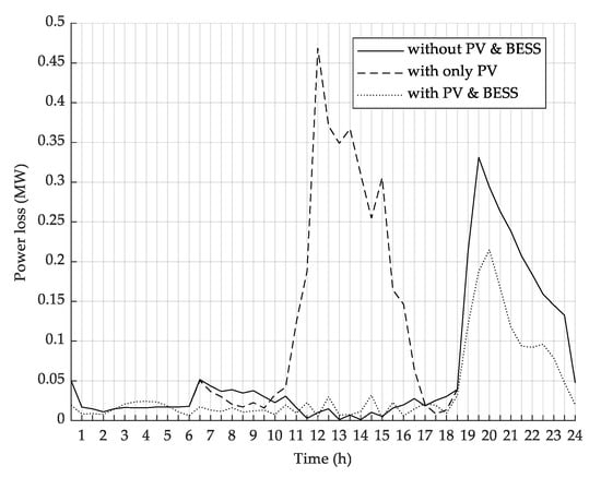
Figure 9.
Real power loss comparison of three cases.
5.4. Peak Demand
The peak demand, which is the peak real power demand, at the slack bus over 24 h is depicted in Figure 10. It could be observed that the peak demands of both cases 1 and 3 flowed in only one direction flowing into the network, while the peak demand of case 2 flowed in both directions (into and out from the distribution network). It is found from case 1 that the maximum real power was equal to 6.75 MW at 7:30 p.m. (the 19th hour and a half), which is the highest demand of the day. For case 2, the maximum real power flowing into the distribution network is equal to 6.75 MW at 7:30 p.m. (the 19th hour and a half), which is the same value and hour as case 1, while the maximum reverse power flow is equal to 3.70 MW at 12:00 a.m. (the 12th hour), which is the period of real power supplied by PV. Finally, after the BESS installation in case 3, the real power demand could be maintained within the range of 0–2 MW over 24 h. When compare the peak powers of case 2 and 3, it can be seen that the peak power of case 3 is more than that of case 2 during 2:30 a.m.–5:00 a.m. and 8:00 a.m.–6:00 p.m. This means the BESS was charging during these periods, which matches with Figure 7 when the SoE of the BESS was increased. For the other periods when the peak demand of case 3 is less than that of case 2, it means the BESS was discharging to the network, which can be observed from Figure 7, when the SoE of the BESS was decreased. Thus, the capacity of the BESS significantly depends on the PV power and load demand in the distribution network. Moreover, the BESS installation can delay the distribution network improvement to meet the increasing electricity demand in the future.
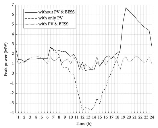
Figure 10.
Peak demand comparison of three cases.
After the BESS installation simulation at the seventh feeder of Nakhon Phanom substation with the connected PV of PEA in Thailand, it is found that the optimal siting and sizing of the BESS installation are at the 47th bus and 4.50 MW/62.72 MWh, respectively, by considering the system cost objective function. It is also found that this siting and sizing of the BESS could significantly improve the performance of the distribution network in terms of voltage deviation improvement, power loss reduction, and peak demand reduction when compared to the cases without BESS installation. By considering the siting of the BESS in the distribution network, it is found that the siting of the BESS affects the system constraints, especially voltage constraints. Only some buses in the network can be selected to install the BESS to improve the voltage profile to be within the standard value. For the sizing of the BESS, the BESS has similar sizes for the BESS installation at different buses in the distribution network. The appropriate size of the BESS of each distribution network depends on the imbalance of supply and demand of that network. Moreover, it could be analyzed that the BESS installation in different siting and sizing results in different performance improvement of the distribution network with the connected PV.
By considering the performance of the distribution network with the connected PV after the BESS installation, it is presented that the voltage profile in one day (24 h) was improved and could be maintained within the constrained voltage limits. Hence, the power quality has been enhanced, leading to the reliability improvement of the distribution network. Regarding power loss, the BESS installation could also considerably reduce the power losses in the distribution network, resulting in more profits of DNO from the electricity selling. In addition, the BESS installation could also deal with the inequality problem between supply and demand in the distribution network by storing energy into the BESS when demand is less than supply and supplying energy when demand is more than supply, especially the peak demand time. The benefit of the peak demand reduction for the DNO is to extend the time for planning, improving, and expanding the distribution network to accommodate the increasing electricity demand in the future. Another benefit is to reduce greenhouse gas emissions due to electricity generation from fossil fuels.
The optimal siting and sizing of the BESS introduced in this study could not only improve the performance of the distribution network with the connected PV, but it could also increase profits and improve reliability for the DNO. Moreover, the implementation presented in this research could efficiently provide the optimal siting and sizing of the BESS with the connected PV in the real distribution networks; therefore, it could also be efficiently applied to other real distribution networks with the connected PV or connected RES.
6. Conclusions
In this study, the optimal siting and sizing of the BESS installation in the realistic radial distribution network with the connected PV, which is the seventh feeder at Nakhon Phanom substation in Thailand, is proposed to improve network performance in terms of voltage deviation improvement, power loss reduction, and peak demand reduction. The optimal siting and sizing of the BESS installation were provided by considering minimum objective function value, which is the total costs incurred in the distribution network within a day including voltage regulation cost, real power loss cost, and peak demand cost. The BESS installation was simulated in the seventh feeder of Nakhon Phanom substation, Thailand, and the PSO optimization algorithm was applied to obtain the solution. After the BESS installation, it is found that the voltage profile was improved and within the voltage constraints, resulting in better power quality and more reliability. The real, reactive, and apparent power losses were reduced to be lower than those of the case without the BESS installation. The peak demand, which is the real power demand flowing through the slack bus, was changed to be within the range of 0–2 MW and flowed into the distribution network that is only in one direction during the considered 24 h. It is also found that BESS installation could reduce costs incurred in the distribution network with the connected PV from USD 5418 to USD 1467, resulting in the more income from the electricity selling to the DNO.
From the achieved results, the analysis in economic terms is considered to find if it is worth installing the BESS in the real distribution network, and how long will it take to obtain the benefits in return.
Author Contributions
Conceptualization, P.B., A.S., P.F., and S.K.; software, P.B.; validation, P.B., A.S., and S.K.; formal analysis, P.B. and S.K.; investigation, P.B. and S.K.; resources, P.B.; data curation, P.B.; writing—original draft preparation, P.B. and S.K.; writing—review and editing, P.B., A.S., and S.K.; visualization, P.B.; supervision, A.S. and S.K.; project administration, A.S. All authors have read and agreed to the published version of the manuscript.
Funding
This research was funded by the Provincial Electricity Authority (PEA) of Thailand.
Institutional Review Board Statement
Not applicable.
Informed Consent Statement
Not applicable.
Data Availability Statement
The authors confirm that the data supporting the findings of this study are available within the article.
Acknowledgments
Authors would like to acknowledge Pradit Fuangfoo for his helpful technical discussions.
Conflicts of Interest
The authors declare no conflict of interest.
Appendix A
The system data for the seventh feeder at Nakhon Phanom substation of Provincial Electricity Authority, Thailand, is presented in Table A1.
Table A1.
System data for the seventh feeder at Nakhon Phanom substation in Thailand.
The dynamic load and PV of the seventh feeder at Nakhon Phanom substation of Provincial Electricity Authority, Thailand, is presented in Table A2.
Table A2.
The dynamic load and PV of the seventh feeder at Nakhon Phanom substation in Thailand.
References
- Migliavacca, G.; Rossi, M.; Siface, D.; Marzoli, M.; Ergun, H.; Rodríguez-Sánchez, R.; Hanot, M.; Leclerq, G.; Amaro, N.; Egorov, A.; et al. The Innovative FlexPlan Grid-Planning Methodology: How Storage and Flexible Resources Could Help in De-Bottlenecking the European System. Energies 2021, 14, 1194. [Google Scholar] [CrossRef]
- Onlam, A.; Yodphet, D.; Chatthaworn, R.; Surawanitkun, C.; Siritaratiwat, A.; Khunkitti, P. Power Loss Minimization and Voltage Stability Improvement in Electrical Distribution System via Network Reconfiguration and Distributed Generation Placement Using Novel Adaptive Shuffled Frogs Leaping Algorithm. Energies 2019, 12, 553. [Google Scholar] [CrossRef]
- Trigkas, D.; Ziogou, C.; Voutetakis, S.; Papadopoulou, S. Virtual Energy Storage in RES-Powered Smart Grids with Nonlinear Model Predictive Control. Energies 2021, 14, 1082. [Google Scholar] [CrossRef]
- Carpinelli, G.; Mottola, F.; Proto, D.; Russo, A.; Varilone, P. A Hybrid Method for Optimal Siting and Sizing of Battery Energy Storage Systems in Unbalanced Low Voltage Microgrids. Appl. Sci. 2018, 8, 455. [Google Scholar] [CrossRef]
- Ali, A.Y.; Basit, A.; Ahmad, T.; Qamar, A.; Iqbal, J. Optimizing coordinated control of distributed energy storage system in microgrid to improve battery life. Comput. Electr. Eng. 2020, 86, 106741. [Google Scholar] [CrossRef]
- Giannitrapani, A.; Paoletti, S.; Vicino, A.; Zarrilli, D. Optimal Allocation of Energy Storage Systems for Voltage Control in LV Distribution Networks. IEEE Trans. Smart Grid 2017, 8, 2859–2870. [Google Scholar] [CrossRef]
- Tang, Z.; Liu, J.; Liu, Y.; Huang, Y.; Jawad, S. Risk awareness enabled sizing approach for hybrid energy storage system in distribution network. IET Gener. Transm. Distrib. 2019, 13, 3814–3822. [Google Scholar] [CrossRef]
- Wang, B.; Zhang, C.; Dong, Z.Y. Interval Optimization Based Coordination of Demand Response and Battery Energy Storage System Considering SOC Management in a Microgrid. IEEE Trans. Sustain. Energy 2020, 11, 2922–2931. [Google Scholar] [CrossRef]
- Luo, L.; Abdulkareem, S.S.; Rezvani, A.; Miveh, M.R.; Samad, S.; Aljojo, N.; Pazhoohesh, M. Optimal scheduling of a renewable based microgrid considering photovoltaic system and battery energy storage under uncertainty. J. Energy Storage 2020, 28, 101306. [Google Scholar] [CrossRef]
- Fernandez-Blanco, R.; Dvorkin, Y.; Xu, B.; Wang, Y.; Kirschen, D.S. Optimal Energy Storage Siting and Sizing: A WECC Case Study. IEEE Trans. Sustain. Energy 2016, 8, 733–743. [Google Scholar] [CrossRef]
- Farrag, M.E.A.; Hepburn, D.M.; Garcia, B. Quantification of Efficiency Improvements from Integration of Battery Energy Storage Systems and Renewable Energy Sources into Domestic Distribution Networks. Energies 2019, 12, 4640. [Google Scholar] [CrossRef]
- Wong, L.A.; Ramachandaramurthy, V.K.; Walker, S.L.; Ekanayake, J.B. Optimal Placement and Sizing of Battery Energy Storage System Considering the Duck Curve Phenomenon. IEEE Access 2020, 8, 1. [Google Scholar] [CrossRef]
- Jiang, X.; Jin, Y.; Zheng, X.; Hu, G.; Zeng, Q. Optimal configuration of grid-side battery energy storage system under power marketization. Appl. Energy 2020, 272, 115242. [Google Scholar] [CrossRef]
- Yuan, Z.; Wang, W.; Wang, H.; Yildizbasi, A. A new methodology for optimal location and sizing of battery energy storage system in distribution networks for loss reduction. J. Energy Storage 2020, 29, 101368. [Google Scholar] [CrossRef]
- Zheng, L.; Hu, W.; Lu, Q.; Min, Y. Optimal energy storage system allocation and operation for improving wind power penetration. IET Gener. Transm. Distrib. 2015, 9, 2672–2678. [Google Scholar] [CrossRef]
- Gong, Q.; Wang, Y.; Fang, J.; Qiao, H.; Liu, D. Optimal configuration of the energy storage system in ADN considering energy storage operation strategy and dynamic characteristic. IET Gener. Transm. Distrib. 2020, 14, 1005–1011. [Google Scholar] [CrossRef]
- Liberati, F.; Di Giorgio, A.; Giuseppi, A.; Pietrabissa, A.; Priscoli, F.D. Efficient and Risk-Aware Control of Electricity Distribution Grids. IEEE Syst. J. 2020, 14, 3586–3597. [Google Scholar] [CrossRef]
- Uddin, M.; Romlie, M.F.; Abdullah, M.F.; Tan, C.K.; Shafiullah, G.M.; Bakar, A.H.A. A novel peak shaving algorithm for islanded microgrid using battery energy storage system. Energy 2020, 196, 117084. [Google Scholar] [CrossRef]
- Zhang, B.; Dehghanian, P.; Kezunovic, M. Optimal Allocation of PV Generation and Battery Storage for Enhanced Resilience. IEEE Trans. Smart Grid 2017, 10, 535–545. [Google Scholar] [CrossRef]
- Mukhopadhyay, B.; Das, D. Multi-objective dynamic and static reconfiguration with optimized allocation of PV-DG and battery energy storage system. Renew. Sustain. Energy Rev. 2020, 124, 109777. [Google Scholar] [CrossRef]
- Murty, V.V.S.N.; Kumar, A. Multi-objective energy management in microgrids with hybrid energy sources and battery energy storage systems. Prot. Control. Mod. Power Syst. 2020, 5, 1–20. [Google Scholar] [CrossRef]
- Das, C.K.; Bass, O.; Mahmoud, T.S.; Kothapalli, G.; Mousavi, N.; Habibi, D.; Masoum, M.A. Optimal allocation of distributed energy storage systems to improve performance and power quality of distribution networks. Appl. Energy 2019, 252, 113468. [Google Scholar] [CrossRef]
- Das, C.K.; Bass, O.; Kothapalli, G.; Mahmoud, T.S.; Habibi, D. Optimal placement of distributed energy storage systems in distribution networks using artificial bee colony algorithm. Appl. Energy 2018, 232, 212–228. [Google Scholar] [CrossRef]
- Jayasekara, N.; Masoum, M.A.S.; Wolfs, P.J. Optimal Operation of Distributed Energy Storage Systems to Improve Distribution Network Load and Generation Hosting Capability. IEEE Trans. Sustain. Energy 2016, 7, 250–261. [Google Scholar] [CrossRef]
- Awad, A.S.A.; El-Fouly, T.H.M.; Salama, M.M.A. Optimal ESS Allocation for Load Management Application. IEEE Trans. Power Syst. 2015, 30, 327–336. [Google Scholar] [CrossRef]
- Nick, M.; Cherkaoui, R.; Paolone, M. Optimal Allocation of Dispersed Energy Storage Systems in Active Distribution Networks for Energy Balance and Grid Support. IEEE Trans. Power Syst. 2014, 29, 2300–2310. [Google Scholar] [CrossRef]
- Awad, A.S.A.; El-Fouly, T.H.M.; Salama, M.M.A. Optimal ESS Allocation for Benefit Maximization in Distribution Networks. IEEE Trans. Smart Grid 2017, 8, 1668–1678. [Google Scholar] [CrossRef]
- Nick, M.; Cherkaoui, R.; Paolone, M. Optimal siting and sizing of distributed energy storage systems via alternating direction method of multipliers. Int. J. Electr. Power Energy Syst. 2015, 72, 33–39. [Google Scholar] [CrossRef]
- Nick, M.; Cherkaoui, R.; Paolone, M. Optimal Planning of Distributed Energy Storage Systems in Active Distribution Networks Embedding Grid Reconfiguration. IEEE Trans. Power Syst. 2017, 33, 1577–1590. [Google Scholar] [CrossRef]
- Liu, J.; Chen, Z.; Xiang, Y. Exploring Economic Criteria for Energy Storage System Sizing. Energies 2019, 12, 2312. [Google Scholar] [CrossRef]
- Khaboot, N.; Srithapon, C.; Siritaratiwat, A.; Khunkitti, P. Increasing Benefits in High PV Penetration Distribution System by Using Battery Enegy Storage and Capacitor Placement Based on Salp Swarm Algorithm. Energies 2019, 12, 4817. [Google Scholar] [CrossRef]
- Li, Y.; Vilathgamuwa, M.; Choi, S.S.; Xiong, B.; Tang, J.; Su, Y.; Wang, Y. Design of minimum cost degradation-conscious lithium-ion battery energy storage system to achieve renewable power dispatchability. Appl. Energy 2020, 260, 114282. [Google Scholar] [CrossRef]
- Dhiman, H.S.; Deb, D. Wake management based life enhancement of battery energy storage system for hybrid wind farms. Renew. Sustain. Energy Rev. 2020, 130, 109912. [Google Scholar] [CrossRef]
- Cao, M.; Xu, Q.; Qin, X.; Cai, J. Battery energy storage sizing based on a model predictive control strategy with operational constraints to smooth the wind power. Int. J. Electr. Power Energy Syst. 2020, 115, 105471. [Google Scholar] [CrossRef]
- Wang, B.; Cai, G.; Yang, D. Dispatching of a Wind Farm Incorporated With Dual-Battery Energy Storage System Using Model Predictive Control. IEEE Access 2020, 8, 144442–144452. [Google Scholar] [CrossRef]
- Pham, T.T.; Kuo, T.-C.; Bui, D.M. Reliability evaluation of an aggregate battery energy storage system in microgrids under dynamic operation. Int. J. Electr. Power Energy Syst. 2020, 118, 105786. [Google Scholar] [CrossRef]
- Ganesan, S.; Subramaniam, U.; Ghodke, A.A.; Elavarasan, R.M.; Raju, K.; Bhaskar, M.S. Investigation on Sizing of Voltage Source for a Battery Energy Storage System in Microgrid With Renewable Energy Sources. IEEE Access 2020, 8, 188861–188874. [Google Scholar] [CrossRef]
- Znu, Y.; Liu, C.; Sun, K.; Shi, D.; Wang, Z. Optimization of Battery Energy Storage to Improve Power System Oscillation Damping. In Proceedings of the 2019 IEEE Power & Energy Society General Meeting (PESGM), Atlanta, GA, USA, 4–8 August 2019; Volume 10, pp. 1015–1024. [Google Scholar] [CrossRef]
- Atwa, Y.M.; El-Saadany, E.F. Optimal Allocation of ESS in Distribution Systems With a High Penetration of Wind Energy. IEEE Trans. Power Syst. 2010, 25, 1815–1822. [Google Scholar] [CrossRef]
- Zheng, Y.; Dong, Z.Y.; Luo, F.J.; Meng, K.; Qiu, J.; Wong, K.P. Optimal Allocation of Energy Storage System for Risk Mitigation of DISCOs With High Renewable Penetrations. IEEE Trans. Power Syst. 2014, 29, 212–220. [Google Scholar] [CrossRef]
- Semero, Y.K.; Zhang, J.; Zheng, D. Optimal energy management strategy in microgrids with mixed energy resources and energy storage system. IET Cyber-Physical Syst. Theory Appl. 2020, 5, 80–84. [Google Scholar] [CrossRef]
- Chen, D.; Jing, Z.; Tan, H. Optimal Siting and Sizing of Used Battery Energy Storage Based on Accelerating Benders Decomposition. IEEE Access 2019, 7, 42993–43003. [Google Scholar] [CrossRef]
- Diezmartínez, C. Clean energy transition in Mexico: Policy recommendations for the deployment of energy storage technologies. Renew. Sustain. Energy Rev. 2021, 135, 110407. [Google Scholar] [CrossRef]
- Fan, X.; Liu, B.; Liu, J.; Ding, J.; Han, X.; Deng, Y.; Lv, X.; Xie, Y.; Chen, B.; Hu, W.; et al. Battery Technologies for Grid-Level Large-Scale Electrical Energy Storage. Trans. Tianjin Univ. 2020, 26, 92–103. [Google Scholar] [CrossRef]
- Stecca, M.; Elizondo, L.R.; Soeiro, T.B.; Bauer, P.; Palensky, P. A Comprehensive Review of the Integration of Battery Energy Storage Systems into Distribution Networks. IEEE Open J. Ind. Electron. Soc. 2020, 1, 1. [Google Scholar] [CrossRef]
- Dufo-Lopez, R.; Cortés-Arcos, T.; Artal-Sevil, J.S.; Bernal-Agustín, J.L. Comparison of Lead-Acid and Li-Ion Batteries Lifetime Prediction Models in Stand-Alone Photovoltaic Systems. Appl. Sci. 2021, 11, 1099. [Google Scholar] [CrossRef]
- Henschel, J.; Horsthemke, F.; Stenzel, Y.P.; Evertz, M.; Girod, S.; Lürenbaum, C.; Kösters, K.; Wiemers-Meyer, S.; Winter, M.; Nowak, S. Lithium ion battery electrolyte degradation of field-tested electric vehicle battery cells—A comprehensive analytical study. J. Power Sources 2020, 447, 227370. [Google Scholar] [CrossRef]
- Xiong, R.; Pan, Y.; Shen, W.; Li, H.; Sun, F. Lithium-ion battery aging mechanisms and diagnosis method for automotive applications: Recent advances and perspectives. Renew. Sustain. Energy Rev. 2020, 131, 110048. [Google Scholar] [CrossRef]
- Yuan, W.-P.; Jeong, S.-M.; Sean, W.-Y.; Chiang, Y.-H. Development of Enhancing Battery Management for Reusing Automotive Lithium-Ion Battery. Energies 2020, 13, 3306. [Google Scholar] [CrossRef]
- BloombergNEF. Lithium-Ion Battery Prices. Available online: https://about.bnef.com/blog/behind-scenes-take-lithium-ion-battery-prices/ (accessed on 15 December 2020).
- BloombergNEF. A Behind the Scenes Take on Battery Pack Prices Fall As Market Ramps Up With Market Average At USD156/kWh In 2019. Available online: https://about.bnef.com/blog/battery-pack-prices-fall-as-market-ramps-up-with-market-average-at-156-kwh-in-2019/ (accessed on 31 January 2021).
- Boonluk, P.; Siritaratiwat, A.; Fuangfoo, P.; Khunkitti, S. Optimal Siting and Sizing of Battery Energy Storage Systems for Distribution Network of Distribution System Operators. Batteries 2020, 6, 56. [Google Scholar] [CrossRef]
- Kerdphol, T.; Fuji, K.; Mitani, Y.; Watanabe, M.; Qudaih, Y. Optimization of a battery energy storage system using particle swarm optimization for stand-alone microgrids. Int. J. Electr. Power Energy Syst. 2016, 81, 32–39. [Google Scholar] [CrossRef]
- Kerdphol, T.; Qudaih, Y.; Mitani, Y. Optimum battery energy storage system using PSO considering dynamic demand response for microgrids. Int. J. Electr. Power Energy Syst. 2016, 83, 58–66. [Google Scholar] [CrossRef]
- Saboori, H.; Hemmati, R.; Jirdehi, M.A. Reliability improvement in radial electrical distribution network by optimal planning of energy storage systems. Energy 2015, 93, 2299–2312. [Google Scholar] [CrossRef]
- Shang, C.; Srinivasan, D.; Reindl, T. An improved particle swarm optimisation algorithm applied to battery sizing for stand-alone hybrid power systems. Int. J. Electr. Power Energy Syst. 2016, 74, 104–117. [Google Scholar] [CrossRef]
- Yang, Y.; Bremner, S.; Menictas, C.; Kay, M. Battery energy storage system size determination in renewable energy systems: A review. Renew. Sustain. Energy Rev. 2018, 91, 109–125. [Google Scholar] [CrossRef]
- Rathore, A.; Patidar, N. Optimal sizing and allocation of renewable based distribution generation with gravity energy storage considering stochastic nature using particle swarm optimization in radial distribution network. J. Energy Storage 2021, 35, 102282. [Google Scholar] [CrossRef]
- Çakmak, E.; Önden, I.; Acar, A.Z.; Eldemir, F. Analyzing the location of city logistics centers in Istanbul by integrating Geographic Information Systems with Binary Particle Swarm Optimization algorithm. Case Stud. Transp. Policy 2021, 9, 59–67. [Google Scholar] [CrossRef]
- Liu, M.; Wang, S.; Yan, J. Operation scheduling of a coal-fired CHP station integrated with power-to-heat devices with detail CHP unit models by particle swarm optimization algorithm. Energy 2021, 214, 119022. [Google Scholar] [CrossRef]
- Lu, L.; Han, X.; Li, J.; Hua, J.; Ouyang, M. A review on the key issues for lithium-ion battery management in electric vehicles. J. Power Sources 2013, 226, 272–288. [Google Scholar] [CrossRef]
- Tan, M.; Gan, Y.; Liang, J.; He, L.; Li, Y.; Song, S.; Shi, Y. Effect of initial temperature on electrochemical and thermal characteristics of a lithium-ion battery during charging process. Appl. Therm. Eng. 2020, 177, 115500. [Google Scholar] [CrossRef]
- MATPOWER—Free, Open-Source Tools for Electric Power System Simulation and Optimization. Available online: https://matpower.org/ (accessed on 24 January 2021).


Publisher’s Note: MDPI stays neutral with regard to jurisdictional claims in published maps and institutional affiliations. |
© 2021 by the authors. Licensee MDPI, Basel, Switzerland. This article is an open access article distributed under the terms and conditions of the Creative Commons Attribution (CC BY) license (http://creativecommons.org/licenses/by/4.0/).