Article

A Novel Data Management Methodology and Case Study for Monitoring and Performance Analysis of Large-Scale Ground Source Heat Pump (GSHP) and Borehole Thermal Energy Storage (BTES) System

1
Department of Mechanical Engineering, Aalto University, 02150 Espoo, Finland
2
College of Urban Construction, Nanjing Tech University, Nanjing 211800, China
*
Author to whom correspondence should be addressed.
Energies 2021, 14(6), 1523; https://doi.org/10.3390/en14061523
Submission received: 28 January 2021 / Revised: 4 March 2021 / Accepted: 7 March 2021 / Published: 10 March 2021
(This article belongs to the Special Issue Advances in Ground Heat Exchangers and Ground-Coupled Heat Pumps)

Abstract

:
Aalto New Campus Complex (ANCC) is a recently inaugurated educational facility at Aalto University, located in Otaniemi (Espoo), Finland. Within over 40,000 m2, it comprises two faculties, a shopping center, recreational areas, and a metro station. ANCC is also a large-scale application of Ground Source Heat Pump (GSHP)–Borehole Thermal Energy Storage (BTES) in Finland, comprising an irregular BTES field of 74 boreholes with an overall length of roughly 23 km and 4 million m3 of energy storage. Therefore, accurate monitoring of the GSHP–BTES energy system is crucial for sustainable and efficient long-term operation. Due to the fundamental issues affecting the accuracy of all thermal energy meters, a novel methodology adjusting for consistency of the measured data (in order to accomplish daily energy balance on both sides of the GSHP) is developed. The proposed methodology is used also in conjunction with reconstruction of missing relevant data before April/May 2020 by applying linear regression techniques. The developed data management is considered essential due to its capability to handle measured data with high uncertainty (thermal meters) by using highly accurate data regarding the GSHP power demand. Additionally, operational data and relevant GSHP performance indicators for the 18-month period starting from July 2019 is presented and analyzed.

1. Introduction

The energy footprint of buildings accounted for 29% of overall primary energy consumption globally in 2018, according to BP Energy Outlook 2020 [1]. In Europe, heating and cooling represent roughly half of all energy used in buildings and industry. As a result, making heating and cooling more sustainable and efficient is a priority for the EU [2]. In this context, ground source heat pumps (GSHP) in tandem with underground thermal energy storage (UTES) is an attractive technological option for efficient dispatching of heating and cooling loads, the integration of renewable energy sources (RES), and waste heat. They are interesting also when aiming for further decarbonization of the existing heating and cooling networks [3,4] and especially effective when applied in a centralized/shared way in a district level [5]. The high potential of GSHP for efficient heating and cooling systems has fomented their exponential deployment and growth during the last decades. This has happened especially between 2015 and 2020 when their utilization almost doubled to 167 TWh/year and the installed capacity increased by 54%, reaching 77.5 GWt [6].
Finland is one of the top leaders in the world in heat pump utilization, with some 900,000 units, of which 140,000 are GSHP [6,7]. However, most of these heat pumps are small units installed in individual dwellings or apartment buildings, with still very few medium-/large-scale realizations. In 2019, Kallio [7] estimated that there were only around 20–25 large-scale GSHP applications in Finland (applications with total borehole length over 10 km).
One of these large-scale GSHP–Borehole Thermal Energy Storage (BTES) successfully operating projects in Finland is the Aalto New Campus Complex (ANCC), with a total borehole length of 23 km powered by a GSHP with installed capacity of 0.8 MWt. The GSHP is the heart of the energy system, providing simultaneously heating and cooling all year round. Therefore, accurate monitoring of the GSHP operation and its interaction with the BTES field is crucial for efficient and sustainable operation in the long-term.
Spitler and Gehlin [8] highlighted the difference between the buildings’ energy performance indicators in the design phase vs. how buildings perform in real conditions, denominated as the “performance gap”. The difficulty in determining the concrete reasons for such a performance gap is an important question raised by Spitler [9]. He considers that measurements and continuous monitoring of the operation of the energy system is essential for identifying the potential problems. There are many factors to be considered, with potential impact on the overall energy performance, such as a building’s envelope and airtightness; quality and correct operation of heating, ventilation, and cooling systems; varying outdoor and indoor conditions (weather, occupancy, etc.); specific parameters related to GSHP–UTES energy systems (e.g., heat pump Coefficient of Performance (COP), source/sink temperatures, balanced interactions between the GSHP and the BTES field, and long-term impact), etc. Moreover, Spitler’s vision of a widespread monitoring network for building performance combined with machine learning and data analytics can improve the operation, can increase the capability of fault detection, and can potentially benefit all implicated stakeholders in the near future [9]. Consequently, the enormous network of all smart meters, data sensors, and measuring devices and the massive amount of data they continuously generate would require a multidisciplinary big data processing environment combined with artificial intelligence algorithms [10].
The increasing interest in evaluating the long-term performance of GSHP operation during the last decades has promoted different approaches such as the SEPEMO scheme (Seasonal PErformance factor and MOnitoring for heat pump systems) [11]. SEPEMO defines four different system boundaries, e.g., the first boundary takes into account Heat Pump (HP) refrigeration cycle, the second one additionally includes the power demand of the circulation pumps on the source-side, the third also takes into account the auxiliary heating and cooling, while the fourth additionally includes the distribution-side circulation pumps and fans [8]. The SEPEMO scheme was primarily developed for noncomplex residential heat pump systems (not specifically GSHPs). Despite the enormous efforts done so far, nowadays, there have been certain limitations of SEPEMO boundaries acknowledged [12], especially when dealing with sophisticated GSHP configurations delivering simultaneously heating and cooling all year round [8,12,13]. Spitler and Gehlin [8] additionally highlighted the complexity to allocate the power demand of the air handling units (AHU) separately to heating, cooling, and ventilation, which for example influences the correct implementation of Seasonal Performance Factor (SPF) boundary 4.
The aim of the present research is to develop and implement a novel data management methodology to assess the performance of a complex GSHP–BTES system, the New Campus Complex of Aalto University, under the conditions of high uncertainty related to measured data. The complexity of such an implementation lies in the delivery of continuous and simultaneous cooling and heating on both sides (evaporator and condenser) of the GSHP while using different heat sources and sinks for balancing the system at the same time: the BTES field acting as both source and sink, and dissipation (heat sink) and district heating (DH) as additional peak heat sources (see Figure 1). The additional challenge related to fundamental issues in the accuracy of all thermal energy meters was accepted as a challenge and a starting point for developing an innovative methodology for measured data management. The consistency of correlated measured data of complex energy systems in buildings has been rarely addressed so far in previous research. Several studies have used measured data to calibrate and optimize building energy simulation models [14,15,16]. However, none of them questioned the accuracy and checked for the consistency of the acquired measured data.
Data validation and reconciliation (DVR) in industrial thermal processes is a technique addressed in several research studies [17,18]. The role of DVR is to extract reliable and accurate information from raw measured data and to produce a consistent dataset resulting in the most probable process operation. DVR belongs to a more general category of data management [17]. The DVR procedure normally intends to correct measurement errors and can be expressed mathematically as an optimization problem for optimally correcting the measurement data in a way that the adjusted values are consistent with the laws of conservation. The objective function is based on the least squares method with various sets of constraints, e.g., in thermal processes—constraints normally based on flow, mass, or energy balance [17].
The novelty of this paper is to introduce a specifically developed DVR methodology for data management adjusting the measured data for consistency in order to achieve the necessary energy balances on both sides of the GSHP. Application of the generalized DVR method, which handles raw measured data with unmeasured quantities (GSHP condenser and evaporator loads), tends to decrease the uncertainty after data reconciliation [17,18] and is a certainly indispensable solution to cope with the inherent high uncertainty of ANCC thermal energy meters. The present work also develops a method for reconstruction of some essential missing measurements before April/May 2020 by applying linear regression techniques based on different correlated measured data (Section 2.5).

2. Materials and Methods

Aalto New Campus Complex and its energy system is introduced in Section 2.1 and Section 2.2 The measurement equipment is described in Section 2.3, and the methodology used for data management is presented in Section 2.4. Additionally, the linear regression models utilized for reconstructing essential missing measured data are presented in Section 2.5.

2.1. Description of the University Complex

Aalto New Campus Complex (ANCC), which was inaugurated in 2018, is located in Otaniemi (Espoo) at 60.186° N/24.825° E, only 10 km from Helsinki. ANCC is a polyfunctional 4/5-storey modern building (Figure 2) and includes the following main parts: the School of Arts, Design, and Architecture (ARTS); the School of Business (BIZ); as well as a shopping center, recreational areas, cafeterias, restaurants, and a metro station (METRO).

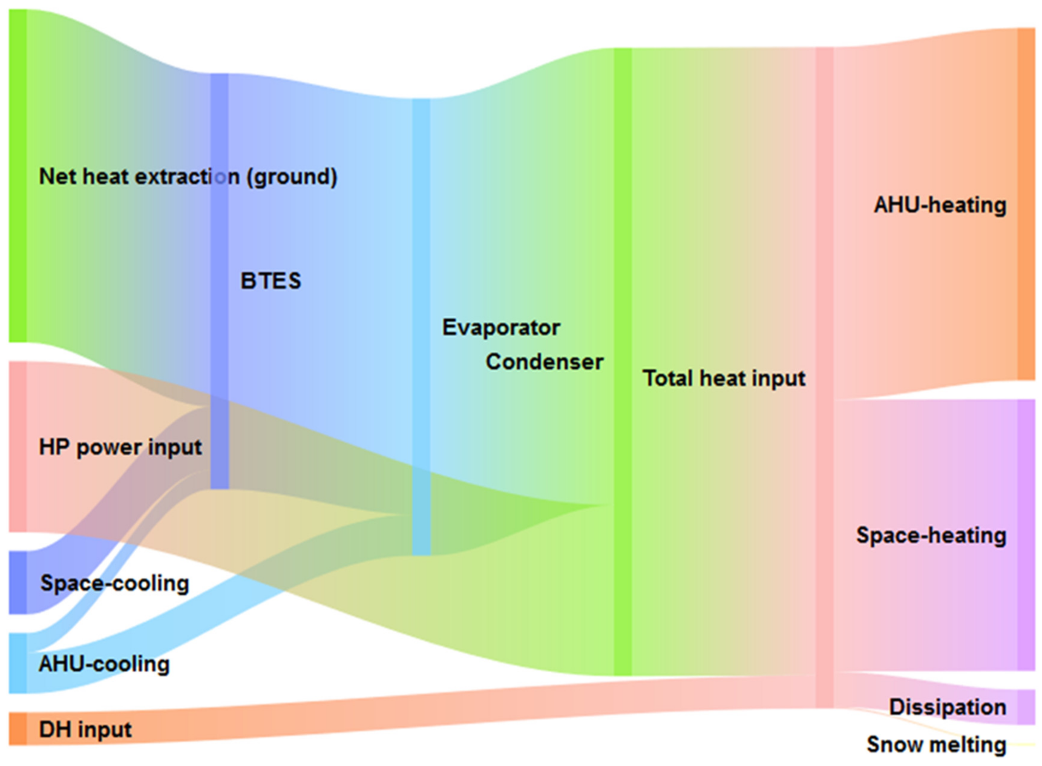
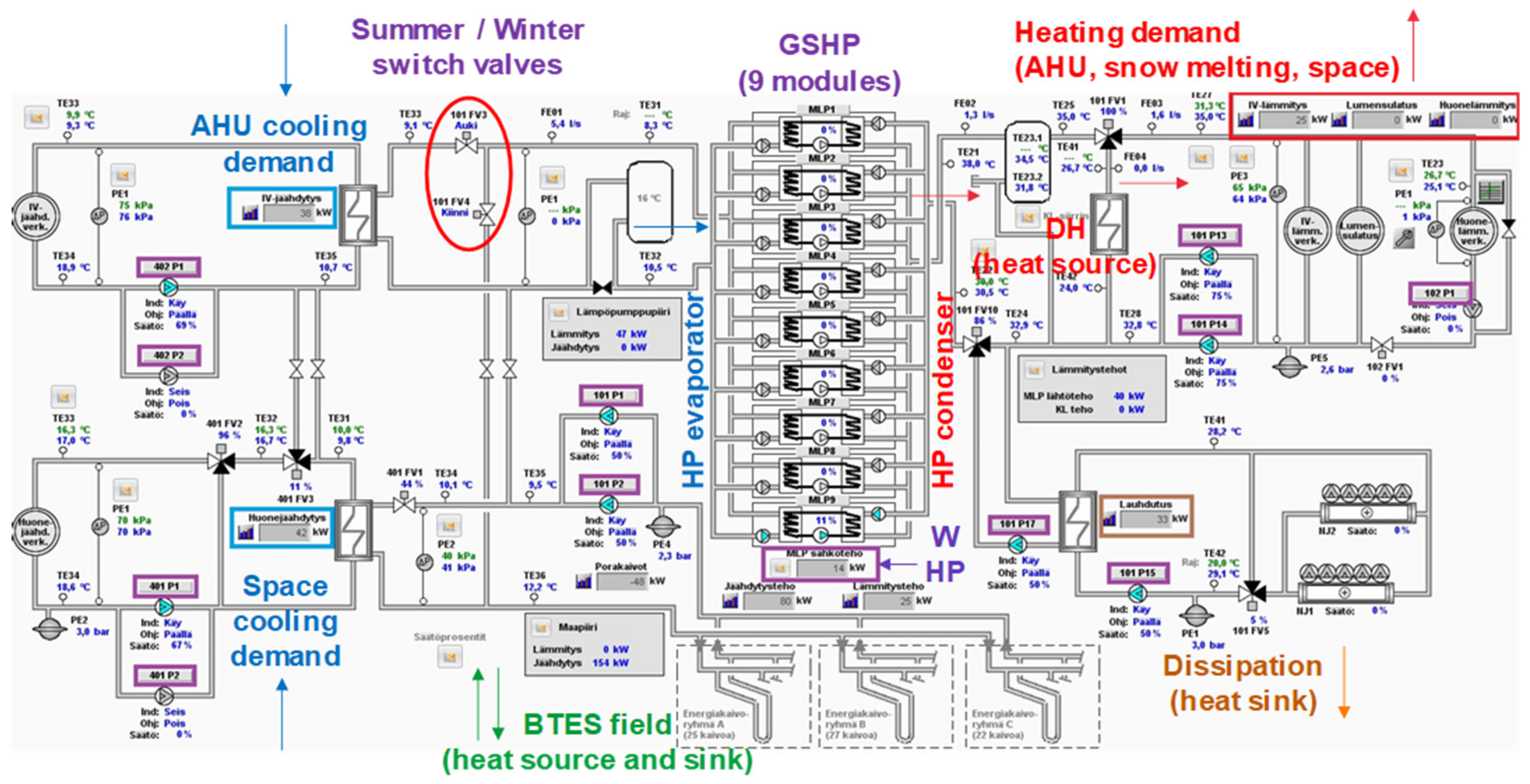
2.2. GSHP–BTES Tandem as Core of the Energy System

The heart of the ANCC energy system is the GSHP, composed of nine centralized heat pump modules operating in a cascade mode, with a total nominal capacity of 790 kW (at brine temperature 0 °C/output temperature 35 °C). Heat pumps generate simultaneously heating on the condenser side and cooling on the evaporator side (Figure 3). Most of the annual cooling demand is delivered as free-cooling energy directly from the boreholes. During the cooling-dominated season (summer), most of AHU-cooling demand is provided directly by the evaporator side of the heat pumps, and at the same time, all waste heat generated on the condenser side is dissipated.
The ground source heat pumps are connected to an irregular BTES field composed of 74 groundwater-filled boreholes with an average effective depth of 302.5 m and a diameter of 115 mm, containing a plastic PE single U-tube pipe with a diameter of 40 mm. The borehole field includes two 11 kW circulation pumps, each one capable of delivering 21 L/s at 200 kPa. Both pumps work in parallel connection by adjusting their output with variable frequency drives (VFD).
Additionally, the energy system is connected to a DH network, which is utilized as a peak heat source in addition to the GSHP. Domestic hot water (DHW) is directly generated by DH; thus, the GSHP is used only for heating. Overall, heating is delivered within a low temperature network (supply temperature 30–45 °C adjusted depending on outdoor temperature) through three different circuits: AHU heating, space heating and snow melting (via embedded pipes in several pedestrian zones). The maximum return temperature is set to 30 °C, and every time it surpasses this value (in summer), excess heat is dissipated. On the other hand, space cooling is provided all year round through radiant systems (supply/return temperatures 12–16 °C/15–18 °C). AHU-cooling operates only with high cooling demand (summer mode) and is provided mostly by an HP evaporator (average supply/return temperatures 10 °C/16 °C). The switching between summer and winter operation depends on several parameters such as the outdoor dry air temperature (ODA), cooling demand, temperatures of the cooling circuits, etc. It occurs normally with an ODA between 12 °C and 15 °C.

2.3. Measurements, Monitoring Equipment, and Performance Indicators

2.3.1. Power Meters

Electrical measurements are usually very accurate (with 0.5–1% accuracy), and this is the case of all power meters within electrical panels, such as the one located in the main Heat, Ventilation, and Air Conditioning (HVAC) mechanical room. All circulation pumps (CP) in the room are controlled by VFD, which also can acquire and measure power demand with an accuracy of 5%. The GSHP power demand is calculated by subtracting all circulation pumps from the overall electricity demand of the main HVAC mechanical room; thus, the measured accuracy of GSHP power demand is around 1–1.5%.

2.3.2. Thermal Energy Meters

Within the monitoring system of ANCC, there are 12 thermal energy meters measuring heating and cooling demand (both AHU- and space-demand) of 3 different zones, namely, the School of Business (BIZ), the Metro station (METRO), and both Schools of Arts and Business (ARTS + BIZ). Additionally, there are 3 thermal energy meters for measuring the BTES field, snow melting, and dissipation energy, respectively. The nomenclature of all thermal energy meters of ANCC is presented in Table 1.
All heating and cooling demands of the ANCC have been monitored since July 2019. However, loads of the BTES field and dissipation have been acquired only since April/May 2020. All thermal energy meters are not calibrated yet, and there is a high uncertainty regarding their measurements due to the following reasons:
  • The accuracy of energy meters depends on different factors: errors related to the flow, sensors’ delta T, calculator, quality of installation, proximity to disturbances and pumps, dirt in fluid, gas entrainment, sampling interval, etc. [19].
  • ANCC meters record data only once per hour regarding flow, temperature, and energy (instead of doing it more frequently, with reduced sampling interval). This can generate significant errors, which are difficult to estimate without calibration.
  • All ANCC meters are battery-powered; thus, the sampling interval can be an issue, since a much longer sample interval is used to reduce power consumption [19]. Meters with slow response can cause significant errors around 20–30% [19].
  • The location of most of the energy meters is far away (sometimes hundreds of meters of pipe connections) from the main HVAC room; thus, heat losses/gains in distribution pipes and heat exchangers are not accounted for and can introduce additional errors.

2.3.3. Seasonal Performance Factors (SPF)

Currently, there is no possibility to separately measure the GSHP compressor and its internal circulation pumps. As mentioned previously, GSHP power demand is monitored as a difference between the overall power demand of the main HVAC room and all circulation pumps. Therefore, considering HP total power demand and the power demand of the BTES circulation pumps, the logical SEPEMO performance metrics is SPF with system boundary 2 [20]. The SPF scheme (boundary 2) considers the net heating and cooling loads covered by the GSHP (plus BTES circulation pumps) and takes into account the free cooling from the ground (e.g., space cooling). Additionally, heat pump COP is calculated as a reference to the refrigeration cycle (the ratio between HP condenser output and HP power input).
The SPF (H2) performance calculation takes into account the HP net heat input to the system (the portion of total heating demand covered by the GSHP). It should be noted that this approach is crucial in the summer, since the GSHP is mostly used to deliver AHU-cooling and only a small fraction of HP condenser supplies net heat to the system (low heat demand); thus, most of HP condenser output has to be dissipated as waste heat. The measured performance for heat pump COP as well as heating, cooling, and combined SPF (boundary 2) is conducted according to the following equations:
C O P   H 1 = Q H P , c o n d W H P
S P F   H 2 = Q n e t _ h e a t W H P , h e a t + W C P , B T E S , h e a t = Q h e a t Q D H , h e a t W H P , h e a t + W C P , B T E S , h e a t
S P F   C 2 = Q c o o l W H P , c o o l + W C P , B T E S , c o o l
S P F   H C 2 = Q c o o l + Q h e a t Q D H , h e a t W H P + W C P , B T E S
where ∑QHP,cond, ∑Qcool, ∑Qheat, ∑QDH,heat, and ∑Qnet_heat are, respectively, the sum of thermal loads over the studied period for HP condenser, total cooling demand, total heating demand, DH input for heating, and total net heating demand (MWh); ∑WHP and ∑WCP,BTES are, respectively, the sum of power demands of the GSHP and BTES circulation pumps (MWh); while additional indices indicate the allocation of power demands for heating and cooling.
During the winter period, all heating loads are considered to be generated by the GSHP (its power demand is allocated only to heating), while power demand of the BTES circulation pumps is allocated proportionally to net heating and cooling loads. In the summer, the GSHP evaporator operates directly against AHU-cooling loads and covers a big share of them (thus, HP power demand is allocated proportionally to the covered AHU-cooling and net heating loads), while the rest of the loads are free-cooling (thus, the power demand of BTES circulation pumps is allocated entirely to space-cooling loads).

2.3.4. Calculation of Heat Pump COP

The measured values of GSHP COP determined with Equation (1) are compared with two different COP estimations based on the source and sink temperatures of the heat pump cycle, namely Lorentz COP [21] and Carnot COP. Reinholdt et al. [21] presented a calculation of Lorentz COPLor, defined as follows:
C O P L o r = η L o r T l m , H T l m , H T l m , L ,   where   T l m , H = T H P C , S T H P C , R l n T H P C , S T H P C , R ;   T l m , L = T H P E , O T H P E , I l n T H P E , O T H P E , I
where Tlm,H and Tlm,L are the logarithmic mean temperatures of the heat pump condenser and evaporator, respectively. THPC and THPE are condenser and evaporator temperatures, while the notation I/O stands for inlet/outlet temperatures of the evaporator and S/R stands for supply/return temperatures of the condenser (expressed in Kelvin). For Lorentz efficiency ηLor, Reinholdt [21] suggested values between 0.5 and 0.6 (for very efficient large-scale heat pumps). A more conservative value of 0.39 was adopted for the ANCC case study.
On the other hand, Carnot COP takes into account only evaporator inlet temperature THPE,I and condenser supply temperature THPC,S, and for ANCC case study, Carnot efficiency ηCar = 0.43 is adopted:
C O P C a r = η C a r T H P C , S T H P C , S T H P E , I

2.4. Measured Data Management through Uncertainty Factors

2.4.1. Uncertainty Factors

A specifically developed DVR procedure with daily resolution is adopted due to the significant thermal inertia of both heating and cooling hydraulic networks, which in practice makes impossible to achieve, e.g., hourly balance on both sides of the GSHP. This resolution is good enough for depicting system daily operation; however, it is not able to capture more precise energy ramping or hourly peak loads.
The proposed particular DVR methodology is used in conjunction with a reconstruction of missing relevant data before April/May 2020 (Section 2.5), allowing for reconstruction of the whole energy system since July 2019. Therefore, the proposed methodology is essential due to its capability to handle measured data with high uncertainty (thermal meters) by using highly accurate data (power meters) as a robust procedure balancing the evaporator and condenser sides of the GSHP.
Four different uncertainty factors were introduced for all measured heating, cooling, BTES, and dissipation loads in order to accomplish a daily balance on both the evaporator and condenser sides of the GSHP.
Relative errors ∆evap,i and ∆cond,i are formulated on both sides of GSHP for each day i of operation:
e v a p , i = Q e v a p , i + Q c o o l , i f c o o l , i + Q B T E S , i f B T E S , i Q e v a p , i ;   c o n d , i = Q c o n d , i + Q D H , i Q h e a t , i f h e a t , i Q d i s s , i f d i s s , i Q c o n d , i
where Qcool,i and Qheat,i are, respectively, total measured cooling demand (negative sign) and total heating demand (positive sign) (MWh); Qevap,i and Qcond,i are the GSHP loads on the evaporator/condenser side (MWh) (positive sign, they are not measured and are determined with the DVR procedure); QDH,i, QBTES,I, and Qdiss,i are the measured loads related to DH (net input for heating, positive sign), BTES (negative for heat extraction from the ground and positive for heat injection), and dissipation (positive sign), respectively, (MWh); and fcool,i, fBTES,i, fheat,i, and fdiss,i are the uncertainty factors for cooling, BTES, heating, and dissipation.

2.4.2. Optimization Problem for Data Management

The optimization problem is defined in order to minimize the sum of squared relative errors ∆evap,i and ∆cond,i (eventually to 0) by varying the aforementioned uncertainty factors fcool,i, fBTES,i, fheat,i, and fdiss,i and the loads on the condenser Qcond,i. It operates with daily values and is formulated on a monthly basis (n is the number of days in a month):
Objective function:
min z = i = 1 n e v a p , i 2 + i = 1 n c o n d , i 2  
Subject to constraints:
  • Q e v a p , i = Q c o n d , i W H P , i , where W H P , i   i s   t h e   G S H P   p o w e r   d e m a n d
  • Q c o n d , i , Q e v a p , i   ,   f c o o l , i   ,   f B T E S , i   ,   f h e a t , i   ,   f d i s s , i ≥ 0 (non-negative condition)
The initial values of all uncertainty factors are set to 1, while the initial values of HP condenser Qcond,i are chosen in order to fulfil the balance on the condenser side (∆cond,i = 0). The optimization problem is solved using the Generalized Reduced Gradient (GRG) nonlinear method in MS Excel Solver.
The obtained uncertainty factors with the optimization procedure are used to adjust the loads by multiplying them with the corresponding uncertainty factors: total cooling demand Qcool,I composed of AHU-cooling QAHU-cool,i and space-cooling Qspa-cool,i; BTES loads QBTES,i; total heating demand Qheat,i composed of AHU-heating QAHU-heat,i, space-heating Qspa-heat,i, and snow melting Qsnow-melt,i; and dissipation loads Qdiss,i. The adjusted data fulfills the necessary energy balances on both sides of the GSHP (evaporator and condenser, which loads are also determined) and therefore is consistent. The detailed procedure applied for data management is depicted in Figure 4.
An illustration of the specific DVR methodology for 12 December 2020 is presented below. The following measured data are obtained (daily loads, in kWh):
  • Evaporator side: Qspa-cool,12 = −1020; QAHU-cool,12 = 0; QBTES,12 = −9345
  • Condenser side: Qspa-heat,12 = 9458; QAHU-heat,12 = 6385; Qsnow-melt,12 = 97; QDH,12 = 655; Qdiss,12 = 0
  • GSHP power demand: WHP,12 = 4360
The initial values of the uncertainty factors are fcool,12 = fBTES,12 = fheat,12 = fdiss,12 = 1. The initial value of GSHP condenser is Qcond,12 = Qspa-heat,12 + QAHU-heat,12 + Qsnow-melt,12QDH,12 + Qdiss,12 = 9458 + 6385 + 97 − 655 + 0 = 15285
After solving the optimization problem, the following results are obtained:
  • fcool,12 = 1.0028; fBTES,12 = 1.0256; fheat,12 = 0.9801; fdiss,12 = 1; Qcond,12 = 14967
The adjusted demands/loads are processed as follows:
  • Qspa-cool,12 = −1020 × 1.0028 = −1023; QAHU-cool,12 = 0 × 1.0028 = 0
  • QBTES,12 = −9345 × 1.0256 = −9584
  • Qspa-heat,12 = 9458 × 0.9801 = 9269; QAHU-heat,12 = 6385 × 0.9801 = 6258; Qsnow-melt,12 = 97 × 0.9801 = 95
  • Qdiss,12 = 0 × 1 = 0
Finally, the evaporator loads are calculated as Qevap,12 = Qcond,12WHP,12 = 14967 − 4360 = 10607. It is possible to check that there are balances on both sides of GSHP:
  • Evaporator: −1023 − 9584 + 10607 = 0
  • Condenser: 14967 + 655 − (9269 + 6258 + 95) − 0 = 0

2.5. Reconstruction of Missing Data Measurements

There are three different types of essential missing data (before April/May 2020) needed to be reconstructed based on different correlated variables: the power demand of all pumps located in the main HVAC room, BTES field interactions (both heat extraction and injection), and dissipation loads (which in the summer have relevant weight in the energy balance of GSHP condenser).

2.5.1. HVAC Pumps

Normally, there are twin pumps in most of the circuits, such as those corresponding to BTES field, heating, and space- and AHU-cooling and dissipation. It was possible to obtain manually the totalized power consumption (kWh) and number of hours of operation for each pump from the automation system within the available period between 13 March 2018 and 16 June 2020 (Table 2).
Table 2 presents a good insight of the system’s operation, and despite its general and limited information, it is possible to draw some valuable conclusions:
  • Pumps of the BTES field account for more than half of the total consumption (51%).
  • All pumps on the BTES and heating circuits are used very intensively for around 64–70% of the time of the studied period, followed by space cooling (44–45%).
  • Pumps on the AHU-cooling circuit (used only during the summer period) are active for around 12% of the time, indicating that summer mode is very short.
  • Dissipation pumps are used very sporadically, only for 4% of the time.
The data with a 5-min resolution for HVAC pumps’ power demand are only available from the middle of April 2020. However, there exists data with a 5-min resolution for the frequency percentage (FP) sent to each pump by the Variable Frequency Drives (VFD), which can be used to restore the missing power demands. The approximate linear correlation between pump power (kW) and the cube of the frequency factor x = (FP/100)3 are well known. Therefore, they are utilized for linear regression based on the data between mid-April and mid-June 2020. The results are shown in Table 3, and considering the weight of each pump within total power demand, the overall standard error is close to 5%. If the outcome of any regression equation turns out to be negative, a minimum value of zero is taken. Using these regression models, missing HVAC pumps’ power demand is reconstructed with an hourly resolution between July 2019 and April 2020.

2.5.2. BTES Field and Dissipation

The energy meter measuring the BTES field started operating properly only since May 21st, 2020. Prior to this, BTES energy data had to be estimated based on the frequency percentage of both pumps (FP1 and FP2) and the difference between flow and return temperature (∆T), as well as by clustering the hourly-based data depending on whether heat is extracted from the ground (negative sign) or injected into to ground (positive sign). The multivariable regression for the BTES field is based on ∆T and the combined frequency factor C F F = F P 1 100 3 + F P 2 100 3 3 , since CFF is approximately proportional to the pumping flow rate of the BTES circuit. The resulting regression equations as well as the corresponding R2 value and the standard error are presented in Table 4. Again, if the outcome is of different sign than expected, a zero value is taken. The high correlations in both regressions (0.94 < R2 < 0.96) are reflected by low standard errors between 13% and 16%.
The energy meter monitoring the dissipated heat started acquiring data only since 23 May 2020. Prior to this, the regression model of dissipation heat rate was based on only one available data point: the entering fluid temperature TE24 within the dissipation internal circuit (Table 4). The outcome can be only nonnegative (thus, for TE24 > 31.8 °C). The lower correlation (R2 = 0.732) implies that the standard error rises to over 42%.

3. Results and Discussion

3.1. Raw Measured Data

The raw measured data were retrieved from the automation system during 18 months between July 2019 and December 2020. All missing data were reconstructed according to the regression models introduced in Section 2.5 (estimations shown in blue font), and the results are presented in Table 5.
From the initially measured data, it is not trivial to determine the evaporator and condenser loads of GSHP, fulfilling the energy balance on both sides of the heat pump. That is why the methodology introduced in Section 2.4 was applied to manage the initial raw data (Table 5) using the introduction of daily uncertainty factors corresponding to cooling, BTES, heating, and dissipation. Consequently, daily loads for cooling, BTES field interaction, heating, and dissipation were adjusted by the corresponding uncertainty factors and shown in Figure 5. Additionally, all daily loads corresponding to GSHP, i.e., evaporator, condenser, and power demand, are presented in Figure 6.
It is interesting that, during the winter period (October to April), the daily heating demand achieves peaks of 20–21 MWh/day and the heat extracted from the ground is 11–12 MWh/day. On the other hand, space cooling is needed all year round (0.5–1 MWh/day), while the intensive use of AHU-cooling in summer (June, July, and August), mostly provided by active HP cooling, can increase the total cooling demand to 14–16 MWh/day. The intensity of summer active cooling (reflected in HP activity, condenser peaks up to 12–14 MWh/day) combined with low heating demand (1.5–2 MWh/day) can provoke daily peaks in dissipation loads up to 12–14 MWh/day.

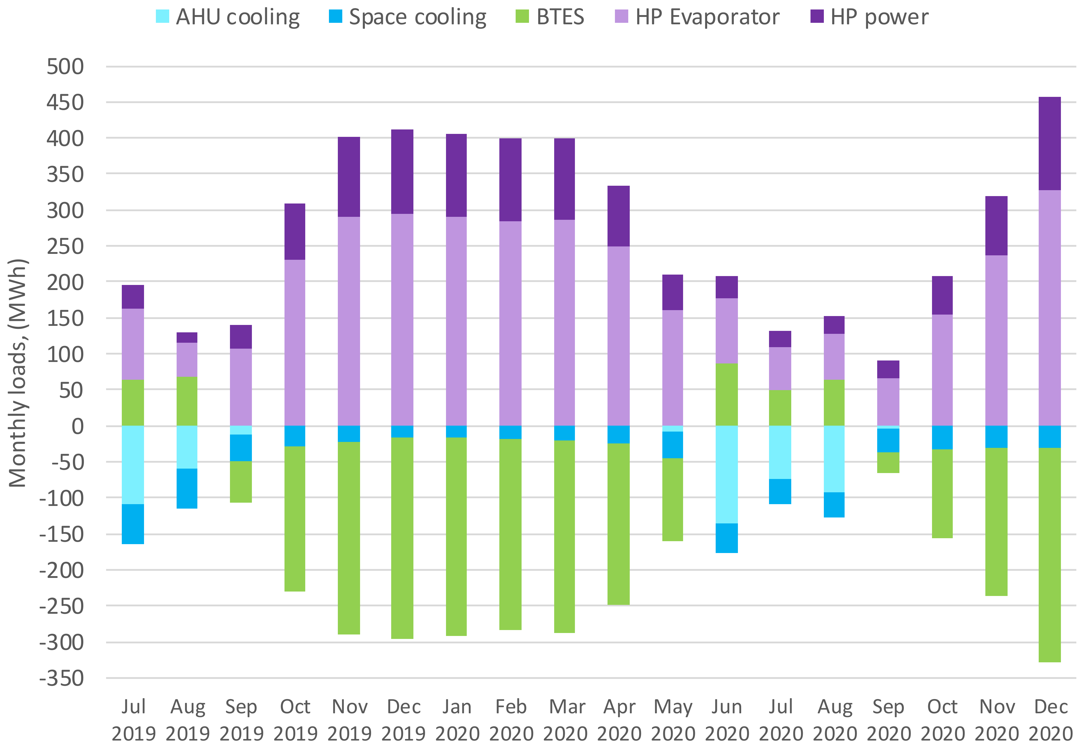
3.2. Results and Analysis of the Evaporator Side

The results of the evaporator side between July 2019 and December 2020 are summarized in Table 6 and Figure 7. The total cooling loads from June to August 2020 account for almost 2/3 of overall annual cooling demand, while AHU-cooling demand over these three months is almost half of annual cooling loads. On the other hand, from October 2019 to April 2020, there is no AHU-cooling demand at all, although space cooling is needed during the whole year. Therefore, it can be concluded that summer operation lasts roughly for three months (June, July, and August) while winter mode covers seven months between October and April, with two transition months in between (May and September).
Similarly, heat from the BTES field is heavily extracted from October 2019 to April 2020 (again, May and September are transition months with lower extraction activity), whereas heat injection occurs during the summer months of June, July and August. Overall, the hourly calculated imbalance ratio during the last 12 months is 7 (1869 MWh heat extraction/268 MWh heat injection). Thus, the interactions with the BTES field are not balanced, which can potentially lead to overcooling in the long term. The uncertainty factors for cooling and BTES are still far from 1 from July to September 2019 and the standard deviation is high (Table 6). After that, they are more stable, i.e., close to 1 and with low standard deviation (due to testing of thermal energy meters, April and May 2020 are exceptions).
The symmetry of Figure 7 also reflects the balance of all loads on the evaporator side. In summer, BTES loads injected into the ground (ground acting as heat sink) plus HP evaporator balance out all cooling loads. For the rest of the year (from September to May), evaporator loads are balanced out by total cooling and BTES loads extracted from the ground (being the ground used as heat source). GSHP power demand in addition to the evaporator loads is also shown in Figure 7 in order to represent the magnitude of HP condenser loads.

3.3. Results and Analysis of the Condenser Side

The monthly loads on the condenser side from July 2019 to December 2020 are presented in Table 7 and Figure 8. In Figure 8, condenser and DH loads are shown as negative in order to highlight the symmetry with all heating and dissipation loads due to the energy balance. As mentioned previously, winter mode can be clearly observed from October 2019 to May 2020, accounting for over 90% of annual heating demand and HP condenser loads. Moreover, space- and AHU-heating demands are more or less evenly distributed over the year, while snow melting is practically inexistent.
As expected, dissipation loads are realized almost entirely during the summer operation in June, July, and August, when they impact hugely on the energy balance of the condenser side (Figure 8). Similar to Figure 7, the symmetry of Figure 8 highlights the energy balance on the condenser side of the heat pump: heat input is provided by the GSHP condenser and DH balanced out by total heating output and dissipation loads (in summer, acting as heat sink). Overall, the GSHP is utilized very intensively, covering some 95% of total annual heat input, with DH accounting only for 5%. However, the past winter (2019–2020) was exceptionally mild in Finland [22]; thus, probably in normal meteorological conditions, the share of DH of overall annual heat input is expected to be higher.
Overall, the uncertainty factors for heating and dissipation are close to 1. However, from July to September 2019, their standard deviation is high (Table 7). After that, the factors are quite stable, close to 1 and with low standard deviation. However, there was testing of all thermal energy meters in April and May 2020 and space-heating metering presented malfunctioning on 5 and 6 July 2020.

3.4. Results and Analysis of the Uncertainty Factors

The initial raw data and the estimations of relevant variables such as BTES field interaction and dissipation can present high uncertainty, which is reflected in the uncertainty factors from July to September 2019, separated from 1 (blue axis) and with wide standard deviation (Figure 9). However, since October 2019, all factors are closer to 1 and have small standard deviation. Again, April and May are exceptions due to continuous testing of all thermal energy meters as are July 5th and 6th, 2020 when there was malfunctioning of space-heat metering (recording negative values). In addition, the BTES circulation pumps were not working for over 20 h.
Therefore, the initial annual period for performance evaluation of the system was selected from October 2019 to September 2020 (highlighted in yellow, Figure 9). During this period, the overall cooling demand, BTES, and HP evaporator loads were 642, 1726, and 2368 MWh, respectively, while HP condenser, total heating demand, DH share for heating, and dissipation loads accounted for 3253, 3242, 171, and 183 MWh, respectively. During this initial period, the imbalance ratio (BTES field) reached the extremely high value of 7.5 (1993 MWh heat extraction/267 MWh heat injection).

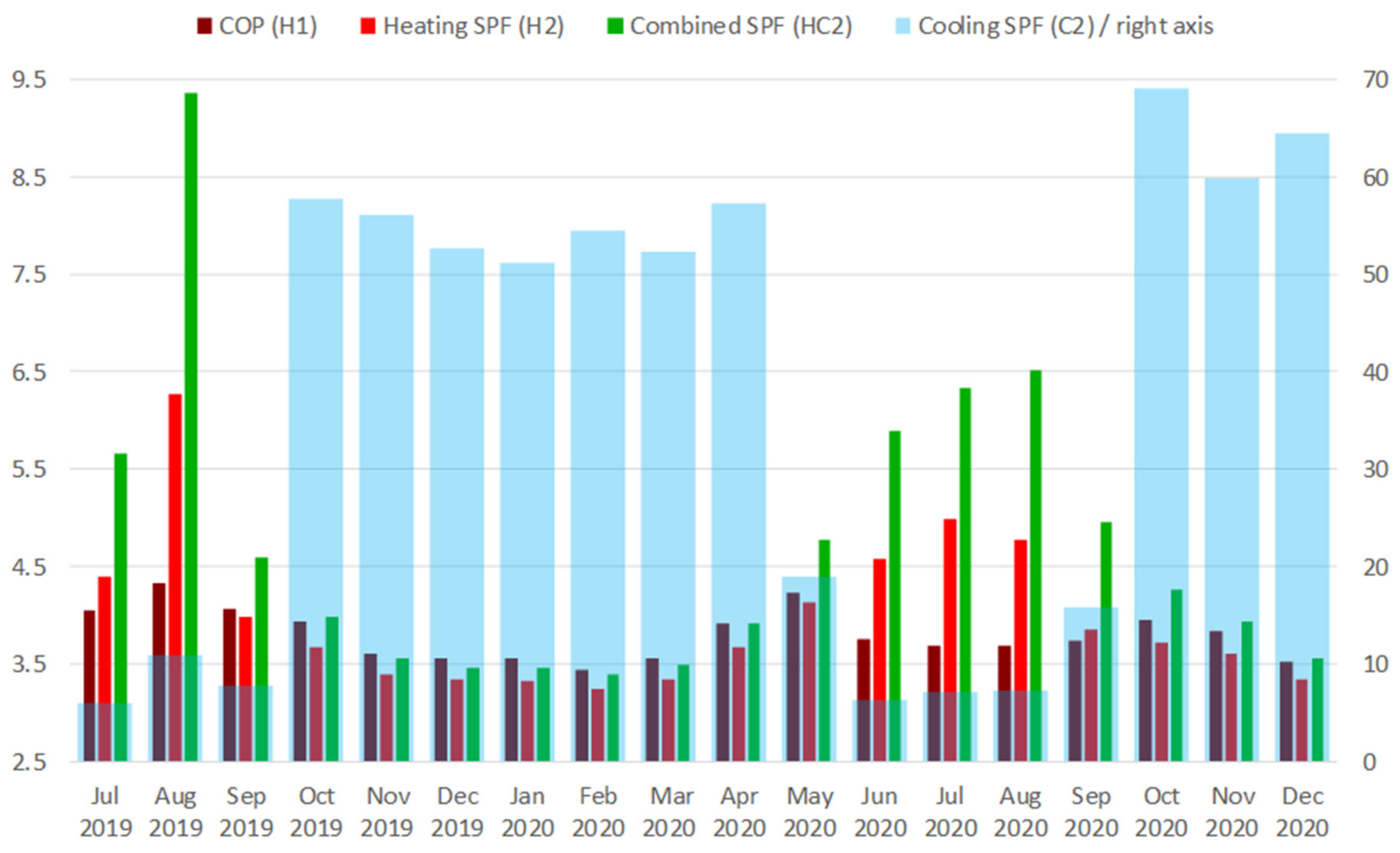
3.5. Performance of the Energy System

Monthly Seasonal Performance Factors (SPF) with SEPEMO boundary 2 were calculated using daily measured data (all thermal loads were adjusted by the uncertainty factors) for the entire period. All heating (SPF-H2), cooling (SPF-C2), and combined SPF-HC2 factors are shown in Figure 10, as is the heating COP (H1).
Cooling SPF factors increase greatly during the winter period (between 50 and 70) due to direct free-cooling from the ground supplied as space-cooling. However, space-cooling demand in winter is a tiny share of annual cooling demand (Figure 7). As expected, winter SPF-H2 is lower than COP(H1) since the former accounts for BTES circulation pumps. The SPF-H2 factor also takes into account the net heating demand, which in winter is a difference between HP condenser and DH input (there is no dissipation), while COP(H1) calculates the heat pump COP (ratio between condenser output and HP power input). During the summer months (June, July, and August) SPF-C2 is lower, between 6.2 and 7.3. Heat pump is intensively utilized to meet almost half of all summer cooling loads, providing active AHU-cooling and simultaneously enhancing the effect of “free heating” on the condenser side. That is why summer SPF-H2 factors are higher than HP COP (Figure 10). Overall, some two-thirds of annual cooling demand is generated by free-cooling (assuming all space-cooling as “free-cooling” provided by the ground source).
The overall heat pump COP and SPF factors for heating, cooling, and combined (system boundary 2) are respectively 3.7, 3.5, 9.3, and 4.0 for the entire period (July 2019–December 2020), while the annualized values over the first evaluation period (October 2019–September 2020) are respectively 3.7, 3.5, 9.3, and 3.9. For comparison, Spitler and Gehlin reported 3.6 and 6.4 as median values for SPF-H2 and C2, respectively, in their exhaustive overview of long-term measured performance of 55 GSHP systems [8]. They also provided values of 3.7 (H2) and 27 (C2) for their own case study: the new student center at Stockholm University in Sweden [8]. The latter factor (C2) is so high because cooling was supplied entirely as free-cooling from the ground peaking in winter between 40 and 60, since source CPs were proportionally allocated to the supplied heating and cooling loads (similarly to the present case study). Another recent study [23] presented an 8/10-year performance of two GSHP–BTES office buildings in Germany, reporting 2.6 and 4 as average SPF H2 and C2, respectively. Similar research for a 4-year GSHP–BTES performance in a German office reported 3.8 and 8 as typical heating SPF H2 and typical cooling SPF C2, respectively [24].

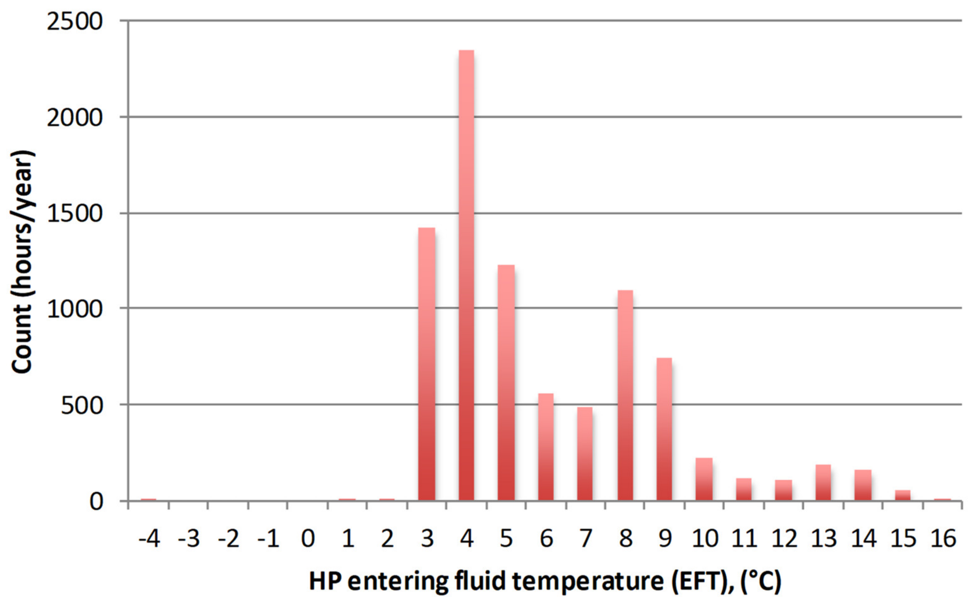
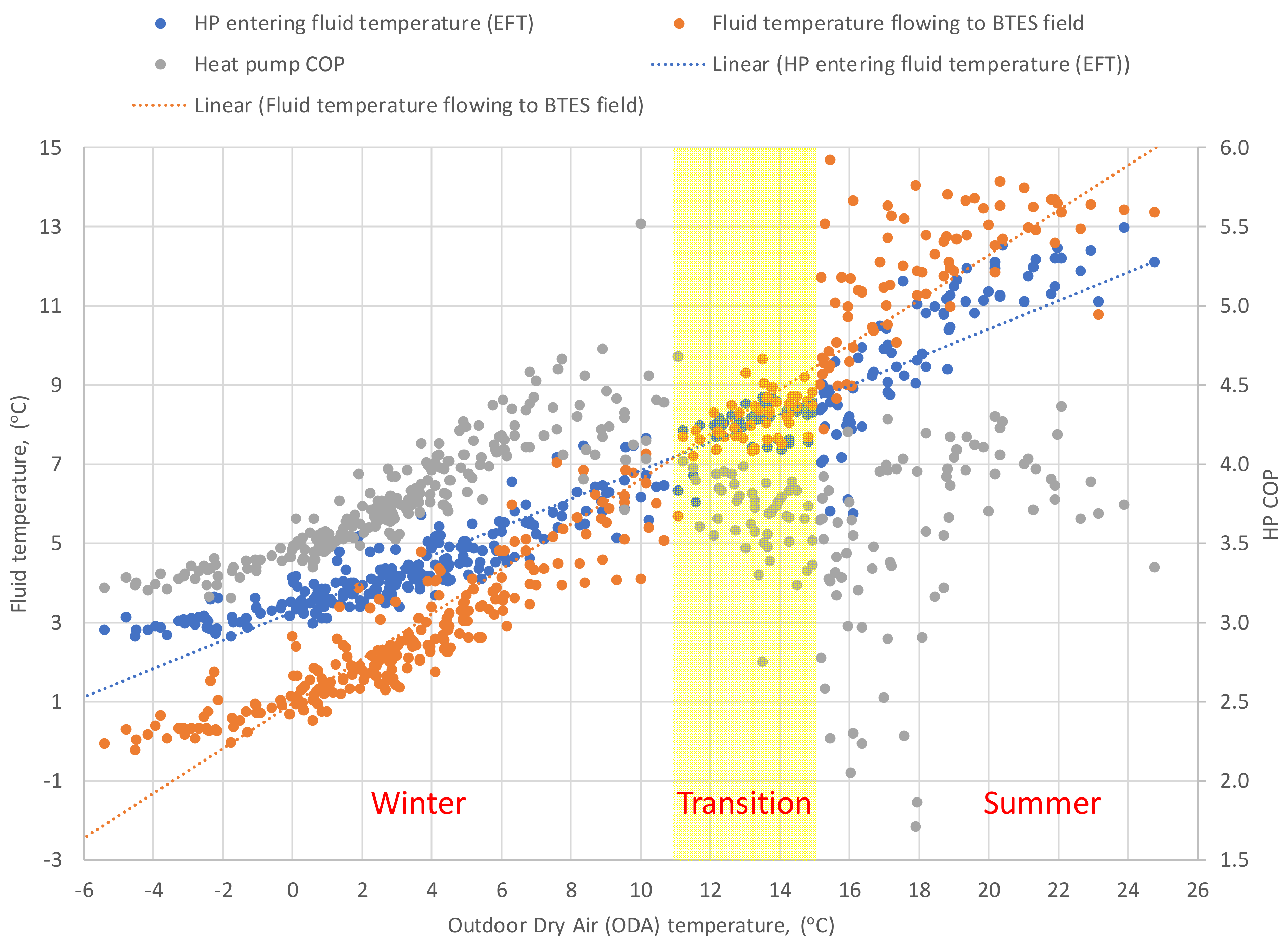
3.6. GSHP Entering Fluid Temperature (EFT)

One of the most important parameters of GSHP’s operation is the entering fluid temperature (EFT) in the evaporator since it reflects how well the BTES field performs and gives a clue about GSHP’s efficiency (since, generally, for a given condenser supply temperature, the higher the EFT, the better the HP COP). The number of hours within the first evaluation period (October 2019–September 2020) with a binned 1 °C HP EFT is presented in Figure 11.
Some 90% of the hours of HP EFT is within a narrow range between 3 and 9 °C, especially from 3 to 5 °C over 60% of the time. It may be normal during the winter period, but in summer operation, more hours with EFT between 10 and 16 °C are expected, since the HP evaporator works directly against the AHU-cooling exchanger.

3.7. Heat Pump COP

Daily values for heat pump fluid temperature vs. outdoor dry air temperature (ODA) are plotted in Figure 12. The HP entering fluid temperature (EFT) and the fluid temperature flowing to the BTES field are compared in the figure.
In winter operation (ODA up to 10–12 °C), the HP evaporator works against the BTES field, and as expected, the EFT is higher than the fluid temperature flowing to BTES (which is the fluid leaving HP evaporator). However, in summer, the HP evaporator operates against the AHU-cooling exchanger and the EFT is consistently lower than the fluid temperature leaving the space-cooling exchanger. The latter confirms our observation that, in summer, the HP evaporator generates AHU-cooling at lower temperatures than necessary, which is also reflected in the heat pump COP (Figure 12), breaking the clearly ascending trend in winter.
It is important to acknowledge also that COP depends on both temperatures on the evaporator side (heat source) and the condenser side (heat sink). The GSHP fluid temperatures on both sides are plotted in Figure 13, where also the measured vs. expected Lorentz/Carnot COP (calculated with equations (5) and (6), ηLor = 0.39/ηCar = 0.43) are compared. Generally speaking, the higher the evaporator temperatures and the lower the condenser temperatures, the higher the COP and vice versa. During the winter period (October 2019–May 2020), the GSHP condenser must provide heating at higher temperatures (average supply/return 42/30 °C) while the intensive heat extraction from the BTES field provokes a temperature drop in the evaporator (average inlet/outlet 4/1 °C). The calculated winter COP (orange line) fits well with the measured COP (green line) showing low plateau with minimum values around 3.5 between November 2019 and March 2020.
On the other hand, in summer operation (June, July, and August 2020), GSHP condenser operates at lower temperatures (average supply/return 36/29 °C) and the evaporator operates at higher temperatures (average inlet/outlet 10/7 °C). This enhances the calculated summer COP to around 5. However, this theoretical expectation is not fulfilled by the measured COP (only 3.7, very similar to the average winter COP), presenting a huge gap between June and September (Figure 13).

3.8. Effect of GSHP Partial Load Operation

The significant gap between the measured COP and expected (calculated) COP in summer operation—as discussed in the previous section—could probably be provoked by the HP partial load operation. Several studies [25,26,27] concluded that heat pump COP is impacted by a partial load operation and highlighted that more frequent “on/off” switching can reduce HP efficiency [25]. As mentioned previously, the ANCC system’s operation is based on cascade launching of HP modules (from 1 to 9 units) and each module can be additionally adjusted to deliver a fraction between 0% and 100% of its nominal capacity. This effect of partial load operation is studied in Figure 14, where 366 daily data points (representing the first evaluation period between October 2019 and September 2020) are plotted depending on the average daily percentage of HP operating modules. Data are additionally clustered in three groups: winter operation (258 days, ODA up to 12–14 °C), summer operation (78 days, ODA over 15 °C), and transition period (30 days, ODA 12–15 °C).
In Figure 14, the average daily COP is plotted on the left axis while the secondary (right) axis shows the average daily ODA temperature (with cruxes). During the winter period, HP COP steadily decreases as modules operate at higher rates (between 25 and 100%). However, it can be seen that COP is closely correlated with ODA temperature, which is expected, since COP is lower with colder weather (during the winter days with high heating demand, EFT is lower and HP supply temperature is higher; thus, COP goes down). In summer, when GSHP modules work at lower capacities, normally up to 30%, COP sharply decreases, especially for an HP capacity below 10–15%. Eventually, a maximum COP (plotted as the decile binned COP, brown line in Figure 14) is achieved between 25% and 50% of HP average capacity, which mostly corresponds to the start/end period of the heating operation (Figure 14, highlighted in yellow).

4. Conclusions

A new methodology for the measured data management of the ANCC energy system was introduced and discussed in the present research. Data acquisition for 18 months, from July 2019 to December 2020, was processed, while essential missing data before April/May 2020 was reconstructed using linear regression techniques.
The presented methodology is considered crucial for tackling the existing uncertainty related to all thermal energy meters difficult to evaluate since they have not been calibrated and has not even been properly commissioned yet. With the introduction of four uncertainty factors related to cooling demand, BTES loads, heating demand, and dissipation, the applied method adjusts all thermal measured data for consistency in order to achieve daily energy balance on both sides of the GSHP and, at the same time, determining the loads of the GSHP evaporator and condenser. It is acknowledged that the aforementioned uncertainty factors present huge spreading with wide standard deviation during the first months (from July to September 2019), implying high uncertainty in the measured/estimated data. After this first period, the uncertainty factors become closer to 1 and their standard deviation steadily decreases. Therefore, the initial annual period for system performance evaluation was selected between October 2019 and September 2020.
The results for all loads on both sides of GSHP (evaporator and condenser) were reported and analyzed for the entire 18-month period, as were HP fluid temperatures, COP, and SPF (for system boundary 2). The HP COP, heating SPF (H2), cooling SPF (C2), and combined SPF (HC2) for the entire period are 3.7, 3.5, 9.3, and 4.0, respectively.
During the initial period for system evaluation (October 2019–September 2020), the corresponding values for HP COP, heating SPF (H2), cooling SPF (C2), and combined SPF (HC2) are 3.7, 3.5, 9.3, and 3.9, respectively. The huge imbalance ratio of 7.5 between the annual heat extracted from and injected into the ground is acknowledged. This can potentially affect sustainable and safe GSHP–BTES operation in the long-term. However, with the current design of the energy system, it is not possible to recover the dissipation waste heat during summer, which would have mitigated the annual excessive heat extraction rate (1.7 GWh/a net heat extraction from the ground) and the potential BTES overcooling in the long-term. Another possible measure to reduce the BTES heat imbalance ratio is by enhancing free-cooling in the summer operation (currently AHU-cooling is mostly generated by active HP cooling).
Additionally, the initial evaluation period is analyzed more thoroughly in terms of heat pump efficiency, i.e., COP dependence on EFT, ODA, and partial load operation. It is concluded that the heat pump EFT maintains below 9 °C for 90% of all hours annually and is particularly low in the summer mode when the HP evaporator operates directly against AHU-cooling. Therefore, higher EFT temperatures between 10 and 16 °C are expected and desirable.
This anomaly during the summer period is apparently related to lower measured heat pump COPs, much lower than the calculated Lorentz/Carnot COPs (measured and calculated COPs actually fit fairly well in winter). However, a closer analysis of HP partial load operation revealed that the heat pump COP drops sharply for an average HP capacity below 25%, which mostly corresponds to summer operation. This drop might also be associated with the increase in parasitic loads at the beginning and end of the summer (daily ODA between 14 and 20 °C) and the transition periods (daily ODA between 12 and 15 °C) when the GSHP has to supply intermittent AHU-cooling loads with more frequent starts and stops. In any case, the detected HP underperformance in the summer should be additionally investigated and corrected.
Overall, the presented novel methodology for measured data management of a sophisticated GSHP–BTES energy system such as Aalto New Campus Complex was proven to be indispensable for overcoming the fundamental issues related to the inherent uncertainty of all thermal energy meters. The proposed approach was certainly essential for the accuracy and confidence of the final results and contributed to estimation of the principal GSHP long-term performance indicators of the energy system. Moreover, the method can potentially be applied in similar complex GSHP systems, simultaneously providing heating and cooling and utilizing various combinations of heat sources and sinks.

Author Contributions

Conceptualization, O.T.; methodology, O.T.; software, O.T.; validation, O.T.; formal analysis, O.T.; investigation, O.T.; resources, O.T. and K.A.; data curation, O.T.; writing—original draft preparation, O.T.; writing—review and editing, O.T. and K.A.; visualization, O.T.; supervision, R.K.; project administration, M.V.; funding acquisition, R.K. and M.V. All authors have read and agreed to the published version of the manuscript.

Funding

This research was funded by Business Finland, grant number 8199/31/2018.

Institutional Review Board Statement

Not applicable.

Informed Consent Statement

Not applicable.

Data Availability Statement

The data are not publicly available due to a confidentiality agreement with Aalto University Campus & Real Estate (ACRE).

Acknowledgments

This research is part of the Smart Otaniemi Project (Aalto University) and contribution to the IEA HPT Annex 52, “Long term performance measurement of GSHP systems serving commercial, institutional, and multi-family buildings”. We highly appreciate the support of Antti Säynäjoki from Aalto University Campus & Real Estate (ACRE).

Conflicts of Interest

The authors declare no conflict of interest.

Abbreviations

AHUAir Handling Unit
ANCCAalto New Campus Complex
BTESBorehole Thermal Energy Storage
CPCirculation Pump
COPCoefficient of Performance
COPCarCarnot COP
COPLorLorentz COP
DHDistrict Heating
DHWDomestic Hot Water
DVRData Validation and Reconciliation
EFTEntering Fluid Temperature (GSHP evaporator)
GRGGSHPGeneralized Reduced GradientGround Source Heat pump
HPHeat Pump
HVACHeat, Ventilation, and Air Conditioning
ODAOutdoor Dry Air Temperature
SPFSeasonal Performance Factor
SEPEMOSeasonal Performance factor and Monitoring for heat pump systems
VFDVariable Frequency Drive
UTESUnderground Thermal Energy Storage

Nomenclature

CFF (-)Combined frequency factor
FP (%)Frequency percentage (pumps)
∑QHP,cond (MWh)Sum of HP condenser loads
∑Qheat (MWh)Sum of total heating demand
∑QDH,heat (MWh)Sum of DH input for heating
∑Qnet,heat (MWh)Sum of total net heating demand
∑Qcool (MWh)Sum of total cooling demand
∑WHP (MWh)Sum of HP power demand (additional indices indicate its allocation for heating
and cooling, respectively)
∑WCP,BTES (MWh)Sum of BTES CP power demand (additional indices indicate its allocation for
heating and cooling, respectively)
fcool,i, fBTES,i (-)Uncertainty factors for total cooling demand and BTES loads
fheat,i, fdiss,i (-)Uncertainty factors for total heating demand and dissipation loads
cond,i (-)Relative error on the condenser side
evap,i (-)Relative error on the evaporator side
Qcond,i (MWh)Daily loads of the condenser (GSHP)
Qevap,i (MWh)Daily loads of the evaporator (GSHP)
Qcool,i (MWh)Measured daily total cooling demand
Qspa-cool,i (MWh)Measured daily space cooling demand
QAHU-cool,i (MWh)Measured daily AHU cooling demand
Qheat,i (MWh)Measured daily total heating demand
Qspa-heat,i (MWh)Measured daily space heating demand
QAHU-heat,i (MWh)Measured daily AHU heating demand
Qsnow-melt,i (MWh)Measured daily snow melting demand
QBTES,I (MWh)Measured daily BTES loads
QDH,i (MWh)Measured daily net DH input for heating
Qdiss,i (MWh)Measured daily dissipation loads
WHP,i (MWh)Measured daily GSHP power demand
WCP,BTES (MWh)Measured daily power demand of BTES circulation pumps
THPE,I/THPE,O (K)HP evaporator inlet/outlet temperature
THPC,S/THPC,R (K)HP condenser supply/return temperature
Tlm,H/Tlm,L (K)HP condenser/evaporator logarithmic mean temperature

References

  1. BP Energy Outlook 2020 Edition. Available online: https://www.bp.com/content/dam/bp/business-sites/en/global/corporate/pdfs/energy-economics/energy-outlook/bp-energy-outlook-2020.pdf (accessed on 13 January 2021).
  2. Communication from the Commission to the European Parliament, the Council, the European Economic and Social Committee and the Committee of the Regions an eu Strategy on Heating and Cooling (COM/2016/051 final). Available online: https://eur-lex.europa.eu/legal-content/EN/TXT/?qid=1575551754568&uri=CELEX:52016DC0051 (accessed on 13 January 2021).
  3. Connolly, D.; Lund, H.; Mathiesen, B.; Werner, S.; Möller, B.; Persson, U.; Boermans, T.; Trier, D.; Østergaard, P.; Nielsen, S. Heat Roadmap Europe: Combining district heating with heat savings to decarbonise the EU energy system. Energy Policy 2014, 65, 475–489. [Google Scholar] [CrossRef]
  4. Todorov, O.; Alanne, K.; Virtanen, M.; Kosonen, R. Aquifer Thermal Energy Storage (ATES) for District Heating and Cooling: A Novel Modeling Approach Applied in a Case Study of a Finnish Urban District. Energies 2020, 13, 2478. [Google Scholar] [CrossRef]
  5. Zhang, Y.; Qi, H.; Zhou, Y.; Zhang, Z.; Wang, X. Exploring the Impact of a District Sharing Strategy on Application Capacity and Carbon Emissions for Heating and Cooling with GSHP Systems. Appl. Sci. 2020, 10, 5543. [Google Scholar] [CrossRef]
  6. Lund, J.W.; Toth, A.N. Direct utilization of geothermal energy 2020 worldwide review. Geothermics 2021, 90, 101915. [Google Scholar] [CrossRef]
  7. Kallio, J. Geothermal Energy Use, Country Update for Finland. Available online: http://europeangeothermalcongress.eu/wp-content/uploads/2019/07/CUR-10-Finland.pdf (accessed on 11 December 2020).
  8. Spitler, J.D.; Gehlin, S. Measured Performance of a Mixed-Use Commercial-Building Ground Source Heat Pump System in Sweden. Energies 2019, 12, 2020. [Google Scholar] [CrossRef] [Green Version]
  9. Spitler, J.D. Addressing the building energy performance gap with measurements. Sci. Technol. Built Environ. 2020, 26, 283–284. [Google Scholar] [CrossRef] [Green Version]
  10. Zhou, K.; Fu, C.; Yang, S. Big data driven smart energy management: From big data to big insights. Renew. Sustain. Energy Rev. 2016, 56, 215–225. [Google Scholar] [CrossRef]
  11. Nordman, R. Seasonal Performance Factor and Monitoring for Heat Pump Systems in the Building SectorSEPEMO-Build. Available online: https://ec.europa.eu/energy/intelligent/projects/sites/iee-projects/files/projects/documents/sepemo-build_final_report_sepemo_build_en.pdf (accessed on 11 January 2021).
  12. Heat Pumping Technologies MAGAZINE-Integration of Heat Pumps into the Future Energy System. Available online: https://issuu.com/hptmagazine/docs/hpt_magazine_no1_2020 (accessed on 25 January 2021).
  13. Naicker, S.S.; Rees, S.J. Performance analysis of a large geothermal heating and cooling system. Renew. Energy 2018, 122, 429–442. [Google Scholar] [CrossRef] [Green Version]
  14. Raftery, P.; Keane, M.; Costa, A. Calibrating whole building energy models: Detailed case study using hourly measured data. Energy Build. 2011, 43, 3666–3679. [Google Scholar] [CrossRef]
  15. Cuerda, E.; Guerra-Santin, O.; Sendra, J.J.; Neila, F.J. Understanding the performance gap in energy retrofitting: Measured input data for adjusting building simulation models. Energy Build. 2020, 209, 109688. [Google Scholar] [CrossRef]
  16. Yang, T.; Pan, Y.; Mao, J.; Wang, Y.; Huang, Z. An automated optimization method for calibrating building energy simulation models with measured data: Orientation and a case study. Appl. Energy 2016, 179, 1220–1231. [Google Scholar] [CrossRef]
  17. Szega, M. Methodology of advanced data validation and reconciliation application in industrial thermal processes. Energy 2020, 198, 117326. [Google Scholar] [CrossRef]
  18. Guo, S.; Liu, P.; Li, Z. Data reconciliation for the overall thermal system of a steam turbine power plant. Appl. Energy 2016, 165, 1037–1051. [Google Scholar] [CrossRef]
  19. Butler, D.; Abela, A.; Martin, C. Heat Meter Accuracy Testing (UK Government, Department for Business, Energy & Industrial Strategy). Available online: https://assets.publishing.service.gov.uk/government/uploads/system/uploads/attachment_data/file/576680/Heat_Meter_Accuracy_Testing_Final_Report_16_Jun_incAnxG_for_publication.pdf (accessed on 15 January 2021).
  20. Zottl, A.; Nordman, R.; Miara, M.; Huber, H. System boundaries for SPF calculation. In Proceedings of the 10th IEA Heat Pump Conference, Tokyo, Japan, 27 June–31 August 2011. [Google Scholar]
  21. Reinholdt, L.; Kristófersson, J.; Zühlsdorf, B.; Elmegaard, B.; Jensen, J.; Ommen, T.; Jørgensen, P.H. Heat pump COP, part 1: Generalized Method for Screening of System Integration Potentials. In Proceedings of the Refrigeration Science and Technology, Valencia, Spain, 18–20 June 2018. [Google Scholar]
  22. Finland Experiencing Mildest Winter in 100 Years. Available online: https://yle.fi/uutiset/osasto/news/finland_experiencing_mildest_winter_in_100_years/11160303 (accessed on 18 January 2021).
  23. Bockelmann, F.; Fisch, M.N. It Works—Long-Term Performance Measurement and Optimization of Six Ground Source Heat Pump Systems in Germany. Energies 2019, 12, 4691. [Google Scholar] [CrossRef]
  24. Luo, J.; Rohn, J.; Bayer, M.; Priess, A.; Wilkmann, L.; Xiang, W. Heating and cooling performance analysis of a ground source heat pump system in Southern Germany. Geothermics 2015, 53, 57–66. [Google Scholar] [CrossRef]
  25. Piechurski, K.; Szulgowska-Zgrzywa, M.; Danielewicz, J. The impact of the work under partial load on the energy efficiency of an air-to-water heat pump. In Proceedings of the E3S Web of Conferences, Boguszów-Gorce, Poland, 23–25 April 2017; EDP Sciences: Les Ulis, France, 2017; Volume 17, p. 72. [Google Scholar]
  26. Watanabe, C.; Ohashi, E.-I.; Hirota, M.; Nagamatsu, K.; Nakayama, H. Evaluation of Annual Performance of Multi-type Air-conditioners for Buildings. J. Therm. Sci. Technol. 2009, 4, 483–493. [Google Scholar] [CrossRef]
  27. Fahlén, P. Capacity control of heat pumps. REHVA J. 2012, 49, 28–31. [Google Scholar]
Figure 1. Annual energy flows (October 2019–September 2020). Total energy input = energy output = 3.4 GWh/a.
Energies 14 01523 g001
Figure 2. General schematics of Aalto New Campus Complex (image courtesy of Tekla, Finland).
Energies 14 01523 g002
Figure 3. Energy system: Heat, Ventilation, and Air Conditioning (HVAC) and Ground Source Heat Pump (GSHP)–Borehole Thermal Energy Storage (BTES) general scheme.
Energies 14 01523 g003
Figure 4. Procedure for data management.
Energies 14 01523 g004
Figure 5. Daily loads after data management procedure.
Energies 14 01523 g005
Figure 6. Daily loads corresponding to GSHP.
Energies 14 01523 g006
Figure 7. Monthly loads on the evaporator side.
Energies 14 01523 g007
Figure 8. Monthly loads on the condenser side.
Energies 14 01523 g008
Figure 9. Uncertainty factors and standard deviation (proportional to the diameter of the bubbles).
Energies 14 01523 g009
Figure 10. Heat Pump (HP) performance: Coefficient of Performance (COP), heating (Seasonal Performance Factor (SPF) H2), cooling (SPF C2), and combined (SPF HC2).
Energies 14 01523 g010
Figure 11. Frequency (hours) for 1 °C binned HP entering fluid temperature (EFT).
Energies 14 01523 g011
Figure 12. Heat pump’s fluid temperature vs. outdoor dry air temperature (ODA) (average daily values).
Energies 14 01523 g012
Figure 13. GSHP evaporator/condenser fluid temperatures and COP.
Energies 14 01523 g013
Figure 14. Heat pump’s COP and ODA in partial load operation.
Energies 14 01523 g014
Table 1. Nomenclature of thermal energy meters in Aalto New Campus Complex (ANCC).
Zone/TypeAHU-CoolingSpace CoolingAHU-HeatingSpace HeatingOthers
ARTS + BIZ402 LM01401 LM01101 LM03102 LM01-
METRO402 LM02401 LM02101 LM04102 LM02-
BIZ402 LM03401 LM03101 LM05102 LM03-
BTES field----101 LM01
Dissipation----101 LM02
Snow melting----191 LM01
Table 2. HVAC pumps: totalized measured data between 13 March 2018 and 16 June 2020.
PumpTypeOverall kWhHours of Operation% of Total DemandAverage Power, kW
101 P1BTES field (1)562351389525.5%4.05
101 P2BTES field (2)570071376125.9%4.14
101 P13Heating circuit (1)231271403210.5%1.65
101 P14Heating circuit (2)233861398810.6%1.67
102 P1Space heating225971274310.3%1.77
401 P1Space cooling (1)1488888226.8%1.69
401 P2Space cooling (2)1352686246.1%1.57
402 P1AHU cooling (1)292621541.3%1.36
402 P2AHU cooling (2)355724731.6%1.44
101 P15Dissipation (external circuit)20328180.9%2.48
101 P17Dissipation (internal circuit)10177970.5%1.28
Table 3. HVAC pumps: parameters for linear regression models and accuracy.
PumpDescriptionNumber of Data PointsRegression Equation (x is the Frequency Factor)R2Standard Error, %
101 P1BTES field (1)22189P (kW) = 7.952x0.9935.4%
101 P2BTES field (2)22189P (kW) = 8.073x0.9945.1%
101 P13Heating circuit (1)17084P (kW) = 5.008x − 0.9770.9054.4%
101 P14Heating circuit (2)17084P (kW) = 4.890x − 0.8730.9054.2%
102 P1Space heating15403P (kW) = 2.049x0.9431.2%
401 P1Space cooling (1)10269P (kW) = 7.346x − 0.9960.8915.7%
401 P2Space cooling (2)10269P (kW) = 7.684x − 0.8600.8606.6%
402 P1AHU cooling (1)5122P (kW) = 11.850x − 2.7670.71910.2%
402 P2AHU cooling (2)5122P (kW) = 11.400x − 2.4840.8379.0%
101 P15Dissipation (ext. c.)2846P (kW) = 7.600x0.9955.1%
101 P17Dissipation (int. c.)2826P (kW) = 4.009x0.9946.6%
Table 4. BTES field and dissipation: Parameters for regression models and accuracy.
DescriptionNumber of Data PointsRegression Equation (CFF is the Combined Frequency Factor, ∆T is Temperature Drop, TE24 is Dissipation Entering Temperature)R2Standard Error, %
BTES field
(heat extraction, negative)
1127 Q (kW) = 152.726 − 208.334∗CFF + 99.957∗∆T0.94516.1%
BTES field
(heat injection, positive)
998 Q (kW) = −166.1 + 285.313∗CFF + 59.382∗∆T0.95913.2%
Dissipation heat507 Q (kW) = −4212.6 + 182.4∗TE24 − 1.569∗TE2240.73242.7%
Table 5. Raw measured data and estimations (blue font).
Month/YearAHU Cooling (MWh)Space Cooling (MWh)Total Cooling (MWh)BTES (MWh)AHU Heating (MWh)Space Heating (MWh)Snow Melting (MWh)Total Heating (MWh)Total DH (MWh)DH for Heating (MWh)DISSIPATION (MWh)HVAC Room (MWhe)Pumps
Power (MWhe)
GSHP Power (MWhe)
Jul 2019−82.9−40.6−123.592.320.825.304635.58.8110.144.111.532.6
Aug 2019−47−44.4−91.3106.318.921.3040.242.18.630.324.31014.3
Sep 2019−9.3−34.3−43.5−47.169.482.20151.649.810.26.74712.334.7
Oct 20190−28.6−28.6−189.9187.1150.30.2337.756.112.20.990.81278.7
Nov 20190−21.9−21.9−251.6266.3180.71.7448.667.423.80.112513.3111.6
Dec 20190−15.4−15.4−263.1264.3185.52.7452.556.320.30128.412.9115.5
Jan 20200−16.1−16.1−259.6250.5186.82439.359.315.7012713.1113.9
Feb 20200−18.4−18.4−249.9270.1176.12.1448.370.726.80128.412.4116.1
Mar 20200−20.4−20.4−252.4258.7171.60.8431.250.314.50124.912.8112.1
Apr 20200−23.6−23.6−203.9211.9160.90.1372.825.9100.196.110.885.3
May 2020−7.3−34.2−41.5−100.4121.1128024926.9100.757.88.149.7
Jun 2020−137.1−40.7−177.886.522.318.4040.832.29.591.640.27.532.7
Jul 2020−74.6−34−108.650.519.233.6052.834.19.639.329.3722.3
Aug 2020−91.6−35−126.665.419.429.7049.134.49.648.830.87.223.6
Sep 2020−4.3−31.5−35.8−27.837.365.40102.739.29.40.430.46.324.1
Oct 2020−0.1−32.2−32.3−119.9114.8108.2022341.110060.98.252.7
Nov 20200−30.4−30.4−200.3150.8188.30339.141.211.3093.710.383.4
Dec 20200−30.8−30.8−291.1199.2301.81.5502.562.6370142.612.8129.9
Table 6. Data management: results of the evaporator side.
Month/YearAverage Outdoor Temp. (°C)AHU Cooling (MWh)Space Cooling (MWh)Total Cooling (MWh)Average Cooling Factors
(±stdev)
BTES (MWh)Average BTES Factors
(±stdev)
Evaporator (MWh)
Jul 201917.9−108.8−54.7−163.51.36 ± 0.2064.30.73 ± 0.2099.5
Aug 201917.0−58.4−57.2−115.71.36 ± 0.4967.90.63 ± 0.1747.8
Sep 201911.4−11.0−38.2−49.21.10 ± 0.15−56.80.92 ± 0.20106.4
Oct 20195.20.0−28.8−28.81.01 ± 0.01−202.01.06 ± 0.03230.8
Nov 20191.90.0−22.0−22.01.00 ± 0.00−268.51.02 ± 0.01290.6
Dec 20191.30.0−15.5−15.51.00 ± 0.00−279.91.06 ± 0.02295.4
Jan 20201.70.0−16.2−16.21.00 ± 0.00−274.71.06 ± 0.02290.9
Feb 20200.30.0−18.5−18.51.00 ± 0.00−265.61.06 ± 0.02284.1
Mar 20201.60.0−20.5−20.51.00 ± 0.00−266.31.06 ± 0.02286.8
Apr 20204.60.0−24.2−24.21.02 ± 0.04−224.71.11 ± 0.04249.0
May 20209.5−7.7−36.7−44.41.07 ± 0.08−116.41.11 ± 0.10160.9
Jun 202018.6−135.1−41.4−176.51.02 ± 0.0786.60.99 ± 0.0489.8
Jul 202016.8−74.6−35.0−109.61.03 ± 0.0749.60.98 ± 0.0560.0
Aug 202017.0−92.0−36.1−128.11.04 ± 0.0764.60.99 ± 0.0463.6
Sep 202012.9−4.5−32.8−37.31.04 ± 0.05−28.61.01 ± 0.0565.9
Oct 20208.3−0.1−32.5−32.61.01 ± 0.01−122.81.03 ± 0.03155.4
Nov 20204.30.0−30.6−30.61.00 ± 0.00−206.11.03 ± 0.02236.7
Dec 20200.80.0−30.9−30.91.00 ± 0.00−297.01.02 ± 0.02327.8
Last 12 months8.0−314−355−6691.02 ± 0.05−16011.04 ± 0.062271
Table 7. Data management: results of the condenser side.
Month/YearCondenser (MWh)AHU Heating (MWh)Space Heating (MWh)Snow Melting (MWh)Total Heating (MWh)Average Heating Factors
(±stdev)
DH for Heating (MWh)Dissipation (MWh)Average Dissipation Factors
(±stdev)
Jul 2019132.119.321.60.040.90.99 ± 0.298.899.80.96 ± 0.07
Aug 201962.119.421.00.040.41.03 ± 0.118.630.41.04 ± 0.19
Sep 2019141.166.478.70.0145.10.97 ± 0.1010.26.71.01 ± 0.07
Oct 2019309.6177.5143.10.2320.90.95 ± 0.0212.20.91.00 ± 0.00
Nov 2019402.2252.6171.71.6425.80.98 ± 0.0223.80.11.00 ± 0.00
Dec 2019410.9251.6177.02.6431.20.96 ± 0.0220.30.01.00 ± 0.00
Jan 2020404.8239.7178.91.9420.40.96 ± 0.0115.70.01.00 ± 0.00
Feb 2020400.2257.1167.92.0427.00.95 ± 0.0226.80.01.00 ± 0.00
Mar 2020398.9248.1164.60.8413.40.96 ± 0.0114.50.01.00 ± 0.00
Apr 2020334.3196.2148.00.1344.30.92 ± 0.0310.00.11.00 ± 0.00
May 2020210.6107.5113.00.0220.50.90 ± 0.0710.10.71.00 ± 0.00
Jun 2020122.521.817.80.039.70.99 ± 0.059.592.31.00 ± 0.01
Jul 202082.319.332.90.052.21.02 ± 0.199.639.61.00 ± 0.01
Aug 202087.219.028.80.047.80.98 ± 0.039.649.01.00 ± 0.01
Sep 202090.036.163.00.099.10.97 ± 0.059.40.41.00 ± 0.00
Oct 2020208.1112.2105.90.0218.10.98 ± 0.0310.00.01.00 ± 0.00
Nov 2020320.1147.5183.90.0331.40.98 ± 0.0211.30.01.00 ± 0.00
Dec 2020457.7196.1297.11.5494.70.98 ± 0.0137.00.01.00 ± 0.00
Last 12 months311716001502631090.97 ± 0.071731821.00 ± 0.00
Publisher’s Note: MDPI stays neutral with regard to jurisdictional claims in published maps and institutional affiliations.

