Comparison of Heat Demand Prediction Using Wavelet Analysis and Neural Network for a District Heating Network

Abstract

Short-Term Load Prediction (STLP) is an important part of energy planning. STLP is based on the analysis of historical data such as outdoor temperature, heat load, heat consumer configuration, and the seasons. This research aims to forecast heat consumption during the winter heating season. By preprocessing and analyzing the data, we can determine the patterns in the data. The results of the data analysis make it possible to form learning algorithms for an artificial neural network (ANN). The biggest disadvantage of an ANN is the lack of precise guidelines for architectural design. Another disadvantage is the presence of false information in the analyzed training data. False information is the result of errors in measuring, collecting, and transferring data. Usually, trial error techniques are used to determine the number of hidden nodes. To compare prediction accuracy, several models have been proposed, including a conventional ANN and a wavelet ANN. In this research, the influence of different learning algorithms was also examined. The main differences were the training time and number of epochs. To improve the quality of the raw data and remove false information, the research uses the technology of normalizing raw data. The basis of normalization was the technology of the Z-score of the data and determination of the energy‒entropy ratio. The purpose of this research was to compare the accuracy of various data processing and neural network training algorithms suitable for use in data-driven (black box) modeling. For this research, we used a software application created in the MATLAB environment. The app uses wavelet transforms to compare different heat demand prediction methods. The use of several wavelet transforms for various wavelet functions in the research allowed us to determine the best algorithm and method for predicting heat production. The results of the research show the need to normalize the raw data using wavelet transforms. The sequence of steps involves following milestones: normalization of initial data, wavelet analysis employing quantitative criteria (energy, entropy, and energy‒entropy ratio), optimization of ANN training with information energy–entropy ratio, ANN training with different training algorithms, and evaluation of obtained outputs using statistical methods. The developed application can serve as a control tool for dispatchers during planning.

1. Introduction

The application of new, progressive technologies to process control is the key to increasing productivity, quality, reliability, and safety [1]. The use of modern process control means predictive control in the management process. It can be achieved by the implementation of artificial intelligence in the control process, together with other data processing methods. This article deals with the problem of short-time (1 h ahead) prediction of energy consumption and planning in heat production, with a comparison of the effectiveness of different methods and algorithms.

Planning is the first phase and is often the most important in many areas. In the area of heat production, the amount of energy produced depends on several variables. The most economical solution would be to produce as much as the demand. This is difficult to achieve in heating systems due to many factors. First, to provide enough heat to the delivery point, it is necessary to produce more heat than is needed. For maximal production efficiency, it is important to make correct decisions. It is convenient to be able to forecast future states and make predictive decisions. The ability to predict is very beneficial generally, such as in systems with high inertia. The control system of a thermal power plant has large inertia in response to changes in the load on the part of customers and will therefore require accurate prediction of the production of the required power and its distribution to individual positions. The current trend in the heating industry is the transition from the third generation to the fourth generation which is characterized by high efficiency, low heat losses, renewable and excess energy utilization. The fourth generation district heating system (DHS) also presents concept that uses low supply temperature which significantly reduces DHS inertia. Transition to the fourth generation can be achieved through the intelligent design of the network—implementing smart meters, smart forecasting algorithm, etc. [2]. District heating is mainly influenced by the demand that means accurate demand prediction is necessary. However, in order to ensure the accuracy of the prediction, it is necessary to include the energy required by the consumers. At present, the accuracy of the predicted behavior of energy consumers is provided by mathematical models, operational statistics, and the experience of dispatchers. This places great demand on dispatcher skills in the production planning process. The use of artificial intelligence opens up new possibilities for improving the accuracy of thermal power plant management and thus increasing the efficiency of energy production. Finally, the improvement of heat load prediction accuracy can ensure the comfort of users and improve energy utilization. The central heating sector can play a significant role in reducing emissions [3] and has an influence on global climate change. It is, of course, also important to consider the availability, environmental friendliness, and price of fuels and the heat transfer medium [4]. The heat consumption originates mainly from heat used for space heating and tap water heating. This combination leads to nonlinearity. It is confirmed that neural networks have ability to solve nonlinearity, and their implementation is successfully proven in many cases and described in many publications [5,6,7].

Besides neural networks, it is possible to use many other methods for short-term prediction. One of them is an application of wavelet transform to analyze data from the predicted process. The aim of this article is a comparison of the prediction accuracy of the mentioned methods. The source was data from the real environment of the heat production company for 2014‒2015, with 2018 used for validation. The local heat plant uses the software TERMIS to optimize heat demand, and the control of the heating process is based on mathematical modeling and statistical methods. Although the data from the environment and heat production are stored in the database, the control of the heating process does not use any method of prediction and is based on mathematical calculations.

The first step is to choose a proper neural network for the creation of the prediction model using data from the heating process. The next steps are the creation of a selected neural network, identifying the data that will be intended for training, testing, and validation, and realization of the learning process itself. After these steps, it is possible to create a software module for predictive control of the heating process.

Similarly, in the second part of this research, the wavelet transform is applied to raw data. First, it is very important to choose a proper method of wavelet transform. Therefore, several wavelet transformations will be computed for different wavelet functions. After these steps, it is possible to make a comparison of different prediction methods for the control of the heating process to choose the best algorithm, whether a neural network or a combination of wavelet transform and neural network.

2. Related Work and Theoretical Basis

This section presents a brief description of the Discrete Wavelet Transform (DWT) and Artificial Neural Networks (ANN) that are used in this research.

2.1. Wavelet Theory and Multiresolution Analysis

Thanks to progress in computer science, there are many cases in which data from time-dependent processes in the physical world were processed using a computer system [8]. There are many algorithms for the better understanding of these processes. The best known and most used is Fourier transform (FT). For computer processing, FT is often paired with Gabor transform, S-transformation, Hilbert transform, or Wavelet transform. In addition to the previously mentioned transformation methods, empirical mode decomposition (EMD) or ensemble empirical mode decomposition (EEMD) are used to solve similar signal processing and surface reconstruction problems [9,10,11]. Wavelet transform and EMD/EEMD are relatively new. The main scope of this contribution is to use wavelet transformation for signal processing, prediction, and to improve the resolution of the data from the controlled process.

Thanks to the work of Meyer and Mallatt [12,13], wavelets have become widely known. Wavelet transform, thanks to its properties, is usable in many fields—mainly picture and video processing [14,15,16,17], fault detection [18,19,20], diagnostics and research in medicine [21,22], but also in many other fields [23,24,25].

Within the management of production processes, a common mathematical task is the prediction of the future state of a system based on known, recorded data. The wavelet transform is not mainly intended as a forecasting technique. It transforms a suspected signal into different levels of resolution and localizes a process in time and frequency. Even so, there are a lot of papers in which it is used in the prediction process.

As we can see from the available literature, wavelet transformation is often used with other technologies, mainly in the process of prediction based on a known system state, data, and parameters from the past. The methods used for the computation of future state differ, including different types of neural network, Nonlinear Least Squares Autoregressive Moving Average (NLS-ARMA) [23,25], high-dimension space mapping [26,27], fractal prediction [28], grey prediction [29], etc. For example, Elarabi et al. [30] proposed an approach that uses both DCT (Discrete Cosine Transform) and DWT (Discrete Wavelet Transform) to enhance the intraprediction phase of H.264/AVC standard. The algorithm presented in their research is designed for video processing software and, according to the authors, extends the benefits of the wavelet-based compression technique to the speed of the FSF algorithm and forms an intraprediction algorithm that ensures a 51% drop in bit rate while keeping the same visual quality and peak signal-to-noise ratio (PSNR) of the original H.264/AVC intraprediction algorithm. A very interesting approach joining wavelet decomposition and adaptive neuro-fuzzy inference system (ANFIS) for ship roll forecasting is described in the work of Li et al. [31].

Stefenon et al. [32] presented an approach to predict the failure of insulators in electric power systems. In their work, they used a hybrid approach with wavelets and neural networks to process data from the ultrasonic scan. Another use of the wavelet method is described in the work of Prabhakar et al. [33]. They describe a combination of Fast Fourier transform (FFT) together with Discrete Wavelet Transform and Discrete Shearlet Transform for predicting surface roughness by milling. The predicted results of the hybrid model were better than the individual transform. The combination of wavelet transform and neural network for prediction is described by Zhang et al. [34]. The core of the article is the creation of a power forecasting model based on dendritic neuron networks in combination with wavelet transform. For decomposing input data in the proposed model, Mallat’s algorithm, which is a fast Discrete Wavelet Transform (DWT), is used. The results show that, with the help of wavelet decomposition, together with various types of neural networks, the prediction process is faster and better compared to the results obtained by the other three conventional models for almost every error criterion.

Another case of joining neural networks with DWT is described in [35]. The article describes the proposal of a hybrid system for prediction that consists of a Long Short-Term Memory (LSTM) neural network and a wavelet module. Wavelet transform is used to decompose the data into a set of subseries, which appears to be very effective. El-Hendawi and Wang [36] describe using a full wavelet packet transform model together with a neural network. Their proposed model is able to predict the electrical load. The model consists of a wavelet packet transform module that is able to decompose a series of high-frequency components into subseries of high and low frequencies. Subseries are fed into the neural networks and the outputs of each neural networks are reconstructed, which is the forecasted load. The described approach is not sensitive to various conditions such as different day types (e.g., weekend, weekday, or holiday) or months. The authors also state that the model can reduce MAPE error by 20% compared to the conventional approach.

Similar problems are solved in [37,38,39]. Tayab et al. [39] propose using wavelet transform with classical feed-forward neural network for short-term forecasting of electricity load demand. Prediction in their work consists of using the best-basis stationary wavelet packet transform. The authors used a Harris hawks optimization to optimize the feed-forward neural network weights. The hybrid model achieved a more than 60% decrease in MAPE compared to SVM and a classical backpropagation neural network. More sophisticated methods are described by Liu et al. [37]. The article predicts wind speed in a wind power generation plant. The highlight is a conjunction of advanced neural network models with wavelet packet decomposition (WPD). The authors developed a new hybrid model to predict wind speed. The model is based on a WPD, convolutional neural network (CNN), and convolutional long short-term memory network (CNNLSTM). In the developed WPD‒CNNLSTM‒CNN model, the WPD is used to decompose the original wind speed time series into various subseries. CNN with a 1D convolution operator is employed to predict the obtained high-frequency subseries and CNNLSTM is employed to complete the prediction of the low-frequency subseries.

The same or a very similar approach to signal processing via wavelet transformation is used in the work of Farhadi et al. [40]. They used a proven procedure of data processing, like other authors. This means that data from the manufacturing process retrieved via piezoelectric sensors and microphones are processed with a combination of wavelet transform and neural network. All calculations are processed by a program written in MATLAB software. The type of neural network used is multilayer perceptron with a backpropagation learning method.

Moreover, wavelet transform, in combination with other algorithms, can be used to filter out noise or interference signals on the premise of ensuring an undistorted original and adding the data prediction function in the data denoising process. Feng et al. [41] described a wavelet-based Kalman smoothing approach for oil well testing during the data processing stage. To improve the dynamic prediction and data resolution, similar approaches with the combination of Kalman prediction and wavelet transform can be found in [42,43]. There is the possibility to use a combination of DWT and other data filters. For example, the most often used method is the common and simple moving average (MA) method [44,45].

It is clear that the wavelet method (DWT) can be widely used for computer data processing in many applications and many scientific fields, together with different technologies, but mainly neural networks. Theory from the area of wavelet transformation is well described in many works [46,47,48,49]. The DWT is considered a linear transformation for which wavelets are discretely sampled. Multiresolution analysis (MRA) and filter bank reconstruction are properties that confirm the wide range of applicability of DWT [50]. The basis functions are derived from a mother wavelet ψ(x), by factors of dilation and translation [51].

$${\psi }_{a,b}\left(x\right)=\frac{1}{\sqrt{a}}\psi \left(\frac{x-b}{a}\right)$$

(1)

where a is the dilation factor and b represents the translation factor. The continuous wavelet transform of a function f(x) can be expressed as follows:

$$F_w\left(a,b\right)=\frac{1}{\sqrt{a}}{{\displaystyle \int }}_{-\infty }^{\infty }f\left(x\right){\psi }^{*}\left(\frac{x-b}{a}\right)dx$$

(2)

where * represents the conjugate operator. The basis functions in (Equation (1)) are redundant when a and b are continuous, so it is possible to discretize a and b to form an orthonormal basis. One way of discretizing a and b is to let a = 2^p and b = 2pq. After this, (Equation (2)) can be expressed as follows:

$${\psi }_{a,b}\left(x\right)=2^{-p/2}{\psi }^{*}\left(2^{-p}x-q\right)$$

(3)

where p and q are integers. Then, the wavelet transform in (Equation (3)) can be expressed as follows:

$$F_w\left(a,b\right)=2^{-p/2}{{\displaystyle \int }}_{-\infty }^{\infty }f\left(x\right){\psi }^{*}\left(2^{-p}x-q\right)dx$$

(4)

where p and q are set to be integers, and it is possible to call (Equation (2)) a wavelet series. It is clear from the representation that the wavelet transform contains both spatial and frequency information. The wavelet transform is based on the concept of multiresolution analysis. That means the signal is decomposed into a series of subsignals and their associated detailed signals at different resolution levels. Generally, these subseries are called approximations (low frequencies) and details (high frequencies). The smooth subsignal (approximation) at level m can be reconstructed from the ith level smooth subsignal and the associated m + 1 detailed signals.

Matlab software is often used for mathematical analysis [52]. Thanks to the number of functions and features, it is suitable for wavelet decomposition, too. The wavelet problem is well managed by the wavelet toolbox.

The principle of the DWT algorithm is depicted in Figure 1, where, after employing the DWT, the procedure comprises of log2 N steps. From signal s, the very first step is to produce two sets of coefficients: approximation coefficients cA1 and detail coefficients cD1. After convolution of the signal s with the lowpass filter LoD and the highpass filter HiD, the dyadic transformation (downsampling) is applied. After obtaining approximation cA1 and detail cD1, the procedure of downsampling continues until the condition of N steps is met. The downsampling procedure is presented in Figure 2.

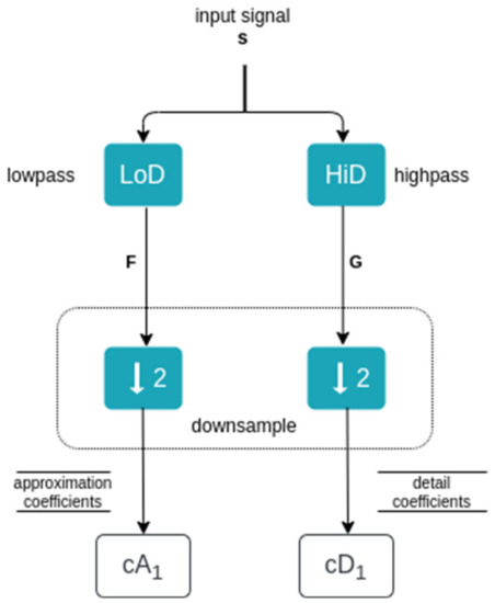
Figure 1. Wavelet decomposition algorithm.

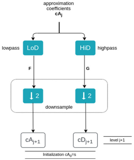
Figure 2. The 1D wavelet decomposition algorithm (wavedec function).

The decomposition was developed by Mallat [12]. DWT is commonly used for fast signal extraction [34]. The decomposition process is iterative, which means that the approximation component after iteration will be decomposed into several low-resolution components.

After the decomposition of the input signal s, we have the low-frequency coefficient cA1 and the high-frequency coefficient cD1 (see Figure 3). After the next decomposition of cA1, high-frequency component cD2 and low-frequency component cA2 are gained. If the decomposition process continues to level j = 3, in the last step coefficients cA3 and cD3 are obtained from cA2. Coefficient cA1 can be reconstructed by cA2 and cD2; similarly, cA2 can be reconstructed by cA3 and cD3.

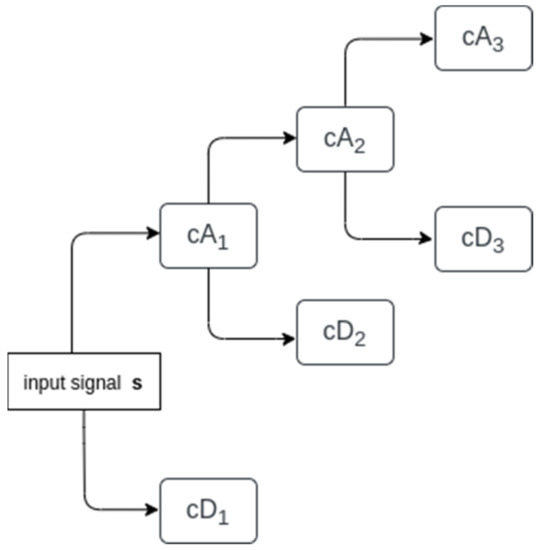
Figure 3. Three-level wavelet decomposition.

The wavelet transform is often used for data preparation for predictive systems with a neural network. In many cases, the type of neural network selected is very simple; oftentimes, a feedforward backpropagation neural network is used.

2.2. Artificial Neural Networks

An artificial neural network can be understood as a parallel processor that tends to preserve the knowledge gained through learning for its future use. They represent an artificial model of the human brain [53]. Knowledge is acquired by neurons during supervised learning, where the relationships between inputs and outputs are mapped. These relationships are created by neurons in the hidden layers that are interconnected. In the hidden layer, neurons capture and extract features from the inputs. The numbers of hidden layers and neurons may be different. Often, the number is selected by a trial-and-error approach, but optimization algorithms can also be used. Input‒output relationships are regulated by weights, which are determined and adjusted during the learning process. The most common learning algorithm is backpropagation (BP). BP consists of two phases: forward and backward. During the forward phase, the response to the inputs is calculated; in the backward phase, the error between the response of the network and desired outputs is calculated. The calculated error is used for adjusting weights between inputs and outputs [54].

The efficiency of the three training algorithms was investigated in this study.

2.2.1. Scaled Conjugate Gradient

The principle of the BP algorithm is based on the calculation and adjustment of the weights in the steepest direction, which is time-consuming. The scaled conjugate gradient (SCG) uses at each iteration a different search direction, instead of the steepest direction that results in the fastest convergence. In the SCG algorithm, the line search technique, which is used to detect the step size, is omitted and replaced by quadratic approximation of the error function (Hessian matrix) together with the trust region from LM. This algorithm requires more iterations to converge but fewer computations between iterations [55].

2.2.2. Levenberg‒Marquardt

The Levenberg‒Marquardt (LM) algorithm was proposed to approach the second-order training speed without computing the Hessian matrix. The LM algorithm offers a tradeoff between the benefits of the Gauss‒Newton method and the steepest descent method. To compute the connection weights wk, the LM uses the following Hessian matrix approximation:

$$w_{k+1}=w_k-{\left[J^T+\mu I\right]}^{-1}{J}^{T}e$$

(5)

where J is the Jacobian matrix (first-order derivatives of the errors), I is the unit matrix, e is the vector of network errors, and $\mu$ is the scalar parameter. Scalar parameter $\mu$ controls the algorithm. If $\mu$ = 0, then the algorithm behaves as in Gauss‒Newton’s method. For a high value of $\mu$, the algorithm uses the steepest descent method [56].

2.2.3. BFGS Quasi-Newton Backpropagation

The BFGS algorithm was proposed by Broyden, Fletcher, Goldfarb, and Shanno. The principle of Newton’s method is based on computing the Hessian matrix. The BFGS algorithm is also based on Newton’s method but uses the approximation of the Hessian matrix; then connection weights $w_k$ are updated via the following Equation:

$$w_{k+1}=w_k-H^{-1}g$$

(6)

where H is the Hessian matrix (second-order derivatives of the errors) and g is the gradient. The BFGS algorithm is computationally more difficult and requires more storage due to computing and storing the approximation of the Hessian matrix [57].

3. Dataset Overview

The input data were provided by the local heating plant, which has more than 300 substations. For our experiments, we used historical load data from 1 November 2014 to 31 March 2015; for that period, we have a mixture of different data from various types of weather (see Figure 4). This dataset is used for training and testing. The total load consists of domestic hot water and the hot water used for central heating. The samples were logged every 10 min. Weather data were also collected from this heating plant. The units for load are in MW and for temperature in °C. Data were downloaded from SCADA in *.xlsx format, and then the data were converted into a suitable format for further processing. A large heat load drop at the beginning of the series was caused by the beginning of the heating season. The statistical characteristics of the data used are presented in Table 1.

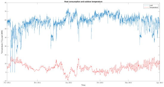
Figure 4. Heat consumption and outdoor temperature.

Table 1. Statistical characteristics of raw data.

Parameter	Min	Max	Mean	Std
Temperature (°C)	−8.93	18.47	5.27	4.52
Load (MW)	0	74.04	32.34	8.92

The scatter plot shown in Figure 5 shows the temperature and load dependency, as well as possible outliers. The presence of outliers can be explained by the fact that, during warmer days, the studied heat plant did not use the maximum power. That means that, during warmer periods, plants with less power were used.

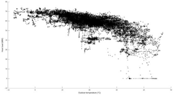
Figure 5. Scatter plot of temperature vs. load.

Data preprocessing is necessary because all these data come from an industrial process, which is often full of errors such as missing data, noisy data, offset, etc. Missing data were substituted by the average of P₋₁ and P₊₁ values. Data normalization is a necessary step to avoid node saturation, which could negatively affect the training phase. For data normalization, we used Z score normalization:

$$Y_i=\frac{X_i-\overline{X}}{\sigma }$$

(7)

where $Y_i$ is the normalized value, $X_i$ is the actual value, $\overline{X}$ is the arithmetic mean, and $\sigma$ is the standard deviation.

4. ANN and WANN Modeling

4.1. Mother Wavelet Selection Criteria

In the past, we can find many papers in the field of heat demand prediction where various researchers applied wavelet transform during the data preprocessing phase to predict heat consumption. The drawback of these studies is that the researchers chose mother wavelet empirically db4 [58], morlet [59]. There is an unwritten rule that Daubechies (db) mother wavelets, especially low order db2–db4, are the most suitable for load forecasting [60,61]. However, each signal has a unique characteristic and therefore we cannot rely on empirical selection. In this section, we are dealing with quantitative methods to select the appropriate mother wavelet. The investigated qualitative methods have different criteria for determining the appropriate mother wavelet; therefore, it is necessary to make a trade-off between criteria.

• Maximum Energy Criteria

The base wavelet that maximizes energy from the wavelet coefficients represents the most appropriate wavelet for the analyzed signal. For a more detailed explanation, see [62].

$$E_{energy} \left(s\right)= {\displaystyle \sum }_{i=1}^N{\left|wt\left(s,i\right)\right|}^2$$

(8)

where N is the number of wavelet coefficients and wt(s,i) corresponds to the wavelet coefficients.

2.

Minimum Shannon Entropy

The base wavelet that minimizes entropy from the wavelet coefficients represents the most appropriate wavelet for the analyzed signal. For a more detailed explanation, see [62].

$$E_{entropy}\left(s\right)= -{\displaystyle \sum }_{i=1}^N{p}_i·{\log }_2{p}_i$$

(9)

where p_i is the energy probability distribution of the wavelet coefficients, defined as

$$p_i=\frac{{\left|wt\left(s,i\right)\right|}^2}{E_{energy}\left(s\right)}$$

(10)

3.

Energy-to-Shannon Entropy ratio

The base wavelet that has produced the maximum energy-to-Shannon entropy ratio was selected to be the most appropriate wavelet for the analyzed signal [62]:

$$R\left(s\right)= \frac{E_{energy\left(s\right)}}{E_{entropy}\left(s\right)}$$

(11)

where E_energy and E_entropy are calculated using (Equations (8) and (9)).

In this section we compared 25 different wavelets from three different wavelet families, namely Daubechies, Symlets, and Coiflets (Figure 6). We also included the haar wavelet, which is often marked as db1. The best wavelet was selected based on the criteria mentioned above. For the first criterion, maximum energy, the best wavelet was db1 or haar. Based on the second criterion, minimum Entropy, the most suitable wavelet was sym 10. This conclusion contradicts the first criterion. To avoid such a conflict, it is necessary to find a trade-off between criteria. Based on the maximum energy‒entropy ratio, the db5 wavelet produced the highest value, which means that that db5 wavelet is the optimal mother wavelet for our purposes.

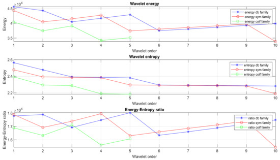
Figure 6. Mother wavelet selection—quantitative criteria.

4.2. Decomposition Level Selection

A suitable decomposition level is as important as selecting the mother wavelet. A high number of decomposition levels might cause information loss, high computational effort, etc. [63]. In the past, several papers were published where researchers used the following empirical equation: L = log₂(N), where N is the series length, to determine the decomposition level [64]. In our case, it would be 14 levels. The difference between the raw heat load series and decomposed series is clearly visible after approximation at level 11. We set the maximum decomposition level to 11; this decomposition level also involves all possible mother wavelet candidates [65]:

$$L= \frac{\log \left(\frac{N}{lw-1}\right)}{\log 2}$$

(12)

where N is the series length and lw is the wavelet filter size.

We focused on a deeper analysis of the decomposed signal via the proposed method by Sang [66]. This method is used to identify the true and noisy components of each decomposition level. The comparison of the energy of raw series and referenced noise series identified components that are close to or inside of the confidence interval of the referenced noise series. In Figure 7, we can clearly identify the components (D1–D3) that are likely to be noise. We suppose that the components above level D4 are true components of the signal. From this analysis, we propose two suitable decompositions at level 6 and level 9 by db5 mother wavelet.

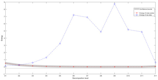
Figure 7. Energy of subseries.

4.3. Building WANN and ANN Models

For an accurate forecast of heat consumption, it is necessary to make a detailed analysis of the variables that influence heat consumption. Generally, energy consumption depends on many factors such as social and climate parameters, type of consumers, etc. Heat demand strongly depends on the outdoor temperature and other climate factors like humidity, wind speed, and so on. Research papers from the past confirm that the strongest influence on demand is outdoor temperature [67]. That fact is also proven by a correlation analysis between heat load and outdoor temperature, where the correlation coefficient is ‒0.78, which could be considered a strong relationship. Another good predictor is historical load. It is likely that consumption the following day at the same time will be similar to the consumption the day before. Significant lags were determined by autocorrelation analysis. Generally, heat load consumption also depends on the time of the day and day of the week. These factors could also increase the prediction accuracy. Table 2 shows the selected input variables for WANN.

Table 2. Selected input variables.

Input Number	Input Name	Value	Calculation
1.	Hour	0–23	Timestamp
2.	Weekend	0–1
3.	Day of the week	1–7
4.	Temperature	Various	Exogenous
5.	Lagged load	Various	Endogenous + timestamp

• Hour—To capture the cyclical behavior of the series, the hour variable was encoded via sine and cosine transform:

$$Hsin=\frac{\sin \left(2\pi h\right)}{24}$$

(13)

$$Hcos=\frac{\cos \left(2\pi h\right)}{24}$$

(14)

Weekend—1 represents weekends and 0 represents weekdays.

Day of the week (DoW)—determines the days of the week, where Mondays are marked as 1 and Sundays as 7.

$$DOWsin= \frac{\sin \left(2\pi dow\right)}{7}$$

(15)

$$DOWcos= \frac{\cos \left(2\pi dow\right)}{7}$$

(16)

Temperature T(t)—The temperature values at lags t, t₋₁₄₄. Because of small differences in temperature, the average temperature at t₋₁ and t₋₂ is used. Lagged load L(t)—Autocorrelation analysis was used to select the most relevant historical consumption. A window of length 1008 (one week) was considered for selection. Selected lags are listed in Table 3.

Table 3. Selected lags and proposed WANN model structure.

Number	Selected Lags		Model Structure (I × h × o)
	L(t)	T(t)
D1	1–5	–		10 × h × 1
D2	1–4, 6	–		10 ×h × 1
D3	1,2,4,5,6	–		10 × h × 1
D4	1–3,10–12	–		11 × h × 1
D5	1–4,20–24	–		14 × h × 1
D6	1–5, 39–42	✓		18 × h × 1
D7	1–5, 79–81	–		13 × h × 1
D8	1–5, 172–174	–		13 × h × 1
D9	1–5, 319–321	✓		17 × h × 1
A9	1–5	✓		14 × h × 1
A6	1–5	✓		14 × h × 1

Determining a suitable number of hidden neurons and hidden layers is crucial in ANN modeling. Too many hidden neurons could cause overfitting. To avoid overfitting, it is crucial to select an appropriate number of neurons in the hidden layer h. Unfortunately, there is no equation to compute the number of hidden neurons. In most cases, the appropriate number of hidden neurons is determined by trial and error. In our research, the number of hidden neurons was determined by rule of thumb: the number of hidden neurons is two-thirds the size of the input layer [67]. The parameters of the proposed models are presented in Table 4.

Table 4. Parameters of proposed feedforward neural networks.

Model	Parameter	Value
BPNN and WANN	Number of hidden layers	1
	Number of neurons in hidden layer	21 for ANN models Various for WANN; see Table 3
	Number of output neurons	1
	Hidden layer activation function	tansig
	Output layer activation function	purelin
	Data set division train/test	random 80/20 (%)
	Epochs	1000
	Data normalization	mapstd; see (Equation (7))
	Training algorithms	trainlm, trainscg, trainbfg
	Learning rate	0.001
WANN	Decomposition level	6 and 9
	Mother wavelet	db5

The proposed methodology is depicted in Figure 8 and consists of the following steps:

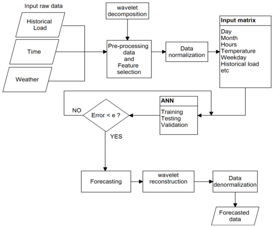
Figure 8. Proposed WANN model flowchart.

• Load input raw data;
• Decompose load data using DWT into N subseries of details and approximations;
• Perform feature selection—autocorrelation, correlation analysis;
• Normalize data using mapstd function;
• Create an input matrix from selected features;
• Divide the processed data into training and testing sets;
• Create WANN models
• Compute the number of hidden neurons (2/3 of inputs)
• Train and test until error starts to increase, then stop training;
• Reconstruct predicted outputs and reconstruct signal X_rec = D₁₊,…,+ D_n + A_n;
• Denormalize outputs using reverse mapstd function;
• Validate proposed models on a new dataset.

5. Results and Discussion

The results of the proposed models for 1 h ahead (10 min sampling interval) are presented in this section. In this research, three FFBP ANNs were proposed and three different learning algorithms, Levenberg‒Marquardt (LM), BFGS quasi-Newton, and Scaled Conjugate Gradient (SCG), were tested. The ANN models were compared with WANNs. The experiments were performed in the MATLAB2020a environment on a laptop with an i7 3.00 GHz CPU and 16 GB memory.

5.1. Evaluation Metrics

To evaluate the accuracy of the proposed models, the following metrics were used: mean absolute error (MAE), mean absolute percentage error (MAPE), and root mean square error (RMSE). The definition of these metrics is as follows:

$$\mathrm{MAE}= \frac{1}{n}{\displaystyle \sum }_{i=1}^n\left|Y_i-\overline{Y_i}\right|$$

(17)

$$\mathrm{MAPE}= \frac{1}{n}{\displaystyle \sum }_{i=1}^n\left|\frac{Y_i-\overline{Y_i}}{Y_i}\right|$$

(18)

$$\mathrm{RMSE}= \sqrt{\frac{1}{n}{\displaystyle \sum }_{i=1}^n{\left(Y_i-\overline{Y_i}\right)}^2}$$

(19)

where n—number of samples, Y_i—actual value, $\overline{Y_i}$—predicted value. The smaller results represent better prediction accuracy.

5.2. WANN and ANN Prediction Comparison

The accuracy of the proposed WANN and ANN models was validated on a dataset from February 2018. This dataset was not included in the training and testing models. Figure 9 and Figure 10 shows the prediction error of the decomposed series with different learning algorithms. Upon visual checking, it is noticeable that the prediction accuracy for the wavelet details D1, D2, and D3 shows high differences compared to other details and there are significant errors according to the other details. The MAPE was 322.93% for LM, and SCG and BFG produced MAPE over 370%. This is caused by high-frequency components (i.e., noise), but these sub-bands also contain some useful features that are predictable. As stated in Section 4.2, sub-bands D1‒D3 contain noise and could be omitted. The error rate rapidly decreases after D4. The presence of a higher error rate is also clearly visible in the A9 series, where BFG and SCG produce much worse predictions compared to the LM algorithm. Both algorithms have a tendency to overestimate the load with the total MAPE for the SCG (0.135%), 0.112% (BFG), and 0.017% (LM). In general, the WANN model shows a good ability to capture the features from the decomposed raw data.

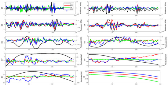
Figure 9. Residuals vs. real load of decomposed series.

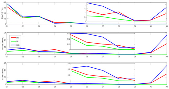
Figure 10. MAPE, RMSE, and MAE performance of the training algorithms.

The error analysis from Figure 10 indicates that the suitable decomposition level is 6. Predicted sub-bands D1, Dn, An were reconstructed to obtain the total heat consumption, which is presented in Figure 11.

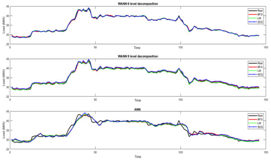
Figure 11. Comparison of reconstructed WANN and ANN (1 h ahead).

The accuracy of the WANNs’ prediction is better compared to conventional ANN. In every experiment, WANN models outperform the conventional ANN model. In each case, the LM algorithm produced the highest accuracy. The MAPE for conventional ANN LM was 1.75%, for WANN LM6 it was 0.359%, and for model WANN LM9 it was 0.362%. The difference between the WANN LM6 and WANN LM9 inaccuracy is negligible. Other values are presented in Table 5 and Figure 12.

Table 5. Errors obtained by ANN and WANN models.

Models	ANN			WANN
Parameters				Dec. Level 6			Dec. Level 9
	BFG	LM	SCG	BFG	LM	SCG	BFG	LM	SCG
MAPE (%)	1.91	1.75	1.83	0.58	0.36	0.51	0.98	0.36	1.51
RMSE (MW)	0.88	0.85	0.89	0.28	0.16	0.25	0.39	0.16	0.56
MAE (MW)	0.66	0.61	0.64	0.20	0.12	0.18	0.33	0.12	0.51

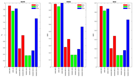
Figure 12. Prediction comparison of different algorithms.

It is worth mentioning that the proposed WANN models in each configuration were able to improve accuracy in every aspect. Percentage improvements are listed in Table 6, which demonstrates the importance of employing DWT in the data preprocessing stage.

Table 6. WANN improvement percentage over conventional ANN.

Improvement percentage	WANN
	Dec. level 6			Dec. level 9
	BFG	LM	SCG	BFG	LM	SCG
MAPE	69%	79%	72%	48%	79%	17%
RMSE	68%	81%	71%	55%	81%	37%
MAE	81%	80%	71%	50%	80%	20%

Table 6 shows that the improvement had a decreasing tendency after decomposition level 6 for the BFG and SCG algorithms. The largest percentage decrease in accuracy was produced by the SCG algorithm in each evaluation metric. The drop was 51% for MAE. However, these decreases in accuracy represented higher overall accuracy compared to conventional ANNs. The LM algorithm produced the biggest improvement in every metric. Compared to the conventional model, the increase was 79%. The LM algorithm showed no improvement after decomposition level 6.

6. Conclusions

This research paper dealt with the prediction of heat consumption. Several models have been created that can predict heat consumption with varying accuracy. Some important findings have been identified during this research. The mother wavelet was chosen based on a quantitative criterion, the energy‒entropy ratio. According to Figure 6, the most suitable mother wavelet was db5. From the presented results, it is clear that the suitable decomposition level is 6. The accuracy of the reconstructed signals shows that models with decomposition level 6 have better results compared to models with decomposition level 9 (Figure 10 and Figure 11). Also, we can state that some details could be omitted during the signal reconstruction. Several models were created for the purpose of finding the most appropriate training algorithm. The presented results show that models trained with an LM algorithm outperform other models (Table 5). Calculation of the error metrics MAPE, RMSE, and MAE proved that the LM training algorithm offered the best results for all models. This research also compared the effectiveness of employing wavelet transform during data preprocessing. In each case, the WANN models predicted heat consumption with significantly higher accuracy compared to ANNs. Significant differences in accuracy were achieved in every WANN model. The LM algorithm produced the highest accuracy among WANN and ANN models. Compared to the conventional model (1.75% MAPE), the improvement was near five times greater (0.36% MAPE). The highest error was produced by the BFG algorithm in both cases. We can state that a combination of wavelet decomposition and ANN could significantly improve the prediction performance. The outcome of this research is also a MATLAB GUI application that could be used by dispatchers. In future research, there are several opportunities to improve the models, e.g., propose and test other ANN architectures like Elman, RNN, optimize the number of hidden neurons with PSO, reduce input parameters with PCA, and propose models with a longer forecasting period (12 h ahead, 24 h ahead).

References

- Gabriska, D. Evaluation of the Level of Reliability in Hazardous Technological Processes. Appl. Sci. 2021, 11, 134. [Google Scholar] [CrossRef]
- Kurek, T.; Bielecki, A.; Świrski, K.; Wojdan, K.; Guzek, M.; Białek, J.; Brzozowski, R.; Serafin, R. Heat Demand forecasting algorithm for a Warsaw district heating network. Energy 2021, 217. [Google Scholar] [CrossRef]
- Guo, B.; Cheng, L.; Xu, J.; Chen, L. Prediction of the Heat Load in Central Heating Systems Using GA-BP Algorithm. In Proceedings of the International Conference on Computer Network, Electronic and Automation (ICCNEA 2017), Xi’an, China, 23–25 September 2017; pp. 441–445. [Google Scholar] [CrossRef]
- GRANRYD Eric. Refrigerating engineering; Royal Institute of Technology: Stockholm, Sweden, 2009; ISBN 978-91-7415-415-3. [Google Scholar]
- Panapakidis, I.P.; Dagoumas, A.S. Day-ahead natural gas demand forecasting based on the combination of wavelet transform and ANFIS/genetic algorithm/neural network model. Energy 2017, 118, 231–245. [Google Scholar] [CrossRef]
- Yan, K.; Li, W.; Ji, Z.; Du, Y.; Qi, M. A Hybrid LSTM Neural Network for Energy Consumption Forecasting of Individual Households. IEEE Access 2019, 7, 157633–157642. [Google Scholar] [CrossRef]
- Nemeth, M.; Borkin, D.; Michalconok, G. The comparison of machine-learning methods XGBoost and LightGBM to predict energy development. In Proceedings of the Computational Statistics and Mathematical Modeling Methods in Intelligent Systems: Proceedings of 3rd Computational Methods in Systems and Software, Zlín, Czech Republic, 10–12 September 2019; Silhavy, R., Silhavy, P., Prokopova, Z., Eds.; Springer: Cham/Basel Switzerland, 2019; Volume 2, pp. 208–215. [Google Scholar] [CrossRef]
- Nemetova, A.; Borkin, D.; Michalconok, G. Comparison of methods for time series data analysis for further use of machine learning algorithms. In Proceedings of the Computational Statistics and Mathematical Modeling Methods in Intelligent Systems: Proceedings of 3rd Computational Methods in Systems and Software, Zlín, Czech Republic, 10–12 September 2019; Silhavy, R., Silhavy, P., Prokopova, Z., Eds.; Springer: Cham/Basel Switzerland, 2019; Volume 2, pp. 90–99. [Google Scholar] [CrossRef]
- Lang, X.; Rehman, N.; Zhang, Y.; Xie, L.; Su, H. Median ensemble empirical mode decomposition. Signal Process. 2020, 176. [Google Scholar] [CrossRef]
- Zuo, G.; Luo, J.; Wang, N.; Lian, Y.; He, X. Decomposition ensemble model based on variational mode decomposition and long short-term memory for streamflow forecasting. J. Hydrol. 2020, 585. [Google Scholar] [CrossRef]
- Yesilli, M.C.; Khasawneh, F.A.; Otto, A. On transfer learning for chatter detection in turning using wavelet packet transform and ensemble empirical mode decomposition. Cirp J. Manuf. Sci. Technol. 2020, 28, 118–135. [Google Scholar] [CrossRef]
- Mallat, S.G. A Theory for Multiresolution Signal Decomposition: The Wavelet Representation; Technical Report; University of Pennsylvania: Philadelphia, PA, USA, 1987. [Google Scholar]
- Meyer, Y. Wavelets, Algorithms & Applications, 1st ed.; SIAM: Philadelphia, PA, USA, 1993. [Google Scholar]
- Sui, K.; Kim, H.G. Research on application of multimedia image processing technology based on wavelet transform. J. Image Video Process. 2019, 24. [Google Scholar] [CrossRef]
- Mahesh, M.; Kumar, T.R.R.; Shoban Babu, B.; Saikrishna, J. Image Enhancement using Wavelet Fusion for Medical Image Processing. Int. J. Eng. Adv. Technol. 2019, 9. [Google Scholar] [CrossRef]
- Shanmugapriya, K.; Priya, D.J.; Priya, N. Image Enhancement Techniques in Digital Image Processing. Int. J. Innov. Technol. Explor. Eng. 2019, 8. [Google Scholar] [CrossRef]
- Kumar, K.; Mustafa, N.; Li, J.; Shaikh, R.A.; Khan, S.A.; Khan, A. Image edge detection scheme using wavelet transform. In Proceedings of the International Computer Conference on Wavelet Active Media Technology and Information Processing (ICCWAMTIP 2014), Chengdu, China, 19–21 December 2014; pp. 261–265. [Google Scholar] [CrossRef]
- Hashim, M.A.; Nasef, M.H.; Kabeel, A.E.; Ghazaly, N.M. Combustion fault detection technique of sparkignition engine based on wavelet packet transform and artificial neural network. Alex. Eng. J. 2020. [Google Scholar] [CrossRef]
- Gharesi, N.; Mehdi Arefi, M.; Razavi-Farb, R.; Zarei, J.; Yin, S. A neuro-wavelet based approach for diagnosing bearing defects. Adv. Eng. Inform. 2020, 46. [Google Scholar] [CrossRef]
- Kou, L.; Liu, C.; Cai, G.; Zhang, Z. Fault Diagnosis for Power Electronics Converters based on Deep Feedforward Network and Wavelet Compression. Electr. Power Syst. Res. 2020, 185. [Google Scholar] [CrossRef]
- Valizadeh, M.; Sohrabi, M.R.; Motiee, F. The application of continuous wavelet transform based on spectrophotometric method and high-performance liquid chromatography for simultaneous determination ofanti-glaucoma drugs in eye drop. Spectrochim. Acta Part A Mol. Biomol. Spectrosc. 2020, 242. [Google Scholar] [CrossRef]
- Győrfi, Á.; Szilágyi, L.; Kovács, L. A Fully Automatic Procedure for Brain Tumor Segmentation from Multi-Spectral MRI Records Using Ensemble Learning and Atlas-Based Data Enhancement. Appl. Sci. 2021, 11, 564. [Google Scholar] [CrossRef]
- Akansu, A.N.; Serdijn, W.A.; Selesnick, W.I. Emerging applications of wavelets: A review. Phys. Commun. 2010, 3. [Google Scholar] [CrossRef]
- Zuo, H.; Chen, Y.; Jia, F. A new C0 layer wise wavelet finite element formulation for the static and free vibration analysis of composite plates. Compos. Struct. 2020, 254. [Google Scholar] [CrossRef]
- Qin, Y.; Mao, Y.; Tang, B.; Wang, Y.; Chen, H. M-band flexible wavelet transform and its application to thefault diagnosis of planetary gear transmission systems. Mech. Syst. Signal Process. 2019, 134. [Google Scholar] [CrossRef]
- Zhao, Z.; Wang, X.; Zhang, Y.; Gou, H.; Yang, F. Wind speed prediction based on wavelet analysis and time series method. In Proceedings of the International Conference on Wavelet Analysis and Pattern Recognition (ICWAPR 2017), Ningbo, China, 9–12 July 2017; pp. 23–27. [Google Scholar] [CrossRef]
- Ren, P.; Xiang, Z.; Shangguan, R. Design and Simulation of a prediction algorithm based on wavelet support vector machine. In Proceedings of the Seventh International Conference on Natural Computation, Shanghai, China, 26–28 July 2011; pp. 208–211. [Google Scholar] [CrossRef]
- Barthel, K.U.; Brandau, S.; Hermesmeier, W.; Heising, G. Zerotree wavelet coding using fractal prediction. In Proceedings of the International Conference on Image Processing (ICIP 1997), Santa Barbara, CA, USA, 26–29 October 1997; Volume 2, pp. 314–317. [Google Scholar] [CrossRef]
- Yin, J.; Gao, C.; Wang, Y.; Wang, Y. Hyperspectral image classification using wavelet packet analysis and gray prediction model. In Proceedings of the International Conference on Image Analysis and Signal Processing (IASP 2010), Zhejiang, China, 9–11 April 2010; pp. 322–326. [Google Scholar] [CrossRef]
- Elarabi, T.; Sammoud, A.; Abdelgawad, A.; Li, X.; Bayoumi, M. Hybrid wavelet—DCT intra prediction for H.264/AVC interactive encoder. In Proceedings of the IEEE China Summit & International Conference on Signal and Information Processing (ChinaSIP 2014), Xi’an, China, 9–13 July 2014; pp. 281–285. [Google Scholar] [CrossRef]
- Li, H.; Guo, C.; Yang, S.X.; Jin, H. Hybrid Model of WT and ANFIS and Its Application on Time Series Prediction of Ship Roll Motion. In Proceedings of the Multiconference on Computational Engineering in Systems Applications (CESA 2006), Beijing, China, 4–6 October 2006; pp. 333–337. [Google Scholar] [CrossRef]
- Stefenon, S.F.; Ribeiro, M.H.D.M.; Nied, A.; Mariani, V.C.; Coelho, L.D.S.; da Rocha, D.F.M.; Grebogi, R.B.; Ruano, A.E.D.B. Wavelet group method of data handling for fault prediction in electrical power insulators. Int. J. Electr. Power Energy Syst. 2020, 123. [Google Scholar] [CrossRef]
- Prabhakar, D.V.N.; Kumar, M.S.; Krishna, A.G. A Novel Hybrid Transform approach with integration of Fast Fourier, Discrete Wavelet and Discrete Shearlet Transforms for prediction of surface roughness on machined surfaces. Measurement 2020, 164. [Google Scholar] [CrossRef]
- Zhang, T.; Chaofeng, L.; Fumin, M.; Zhao, K.; Wang, H.; O’Hare, G.M. A photovoltaic power forecasting model based on dendritic neuron networks with the aid of wavelet transform. Neurocomputing 2020, 397, 438–446. [Google Scholar] [CrossRef]
- Chang, Z.; Zhang, Y.; Chen, W. Electricity price prediction based on hybrid model of Adam optimized LSTM neural network and wavelet transform. Energy 2019, 187. [Google Scholar] [CrossRef]
- El-Hendawi, M.; Wang, Z. An ensemble method of full wavelet packet transform and neural network for short term electrical load forecasting. Electr. Power Syst. Res. 2020, 182. [Google Scholar] [CrossRef]
- Liu, H.; Mi, X.; Li, Y. Smart deep learning based wind speed prediction model using wavelet packet decomposition, convolutional neural network and convolutional long short term memory network. Energy Convers. Manag. 2018, 166, 120–131. [Google Scholar] [CrossRef]
- Xia, C.; Zhang, M.; Cao, J. A hybrid application of soft computing methods with wavelet SVM and neural network to electric power load forecasting. J. Electr. Syst. Inf. Technol. 2018, 5, 681–696. [Google Scholar] [CrossRef]
- Bashir Tayab, U.; Zia, A.; Yang, F.; Lu, J.; Kashif, M. Short-term load forecasting for microgrid energy management system using hybrid HHO-FNN model with best-basis stationary wavelet packet transform. Energy 2020, 203. [Google Scholar] [CrossRef]
- Farhadi, M.; Abbaspour-Gilandeh, Y.; Mahmoudi, A.; Mari Maja, J. An Integrated System of Artificial Intelligence and Signal Processing Techniques for the Sorting and Grading of Nuts. Appl. Sci. 2020, 10, 3315. [Google Scholar] [CrossRef]
- Feng, X.; Feng, Q.; Li, S.; Hou, X.; Zhang, M.; Liu, S. Wavelet-Based Kalman Smoothing Method for Uncertain Parameters Processing: Applications in Oil Well-Testing Data Denoising and Prediction. Sensors 2020, 20, 4541. [Google Scholar] [CrossRef]
- Obidin, M.V.; Serebrovski, A.P. Signal denoising with the use of the wavelet transform and the Kalman filter. J. Commun. Technol. Electron. 2014, 59, 1440–1445. [Google Scholar] [CrossRef]
- Li, Y.J.; Kokkinaki, A.; Darve, E.T.; Kitanidis, P.K. Smoothing-based compressed state Kalman filter for joint state-parameter estimation: Applications in reservoir characterization and CO2 storage monitoring. Water Resour. Res. 2017, 53, 7190–7207. [Google Scholar] [CrossRef]
- Zhang, X.; Ni, W.; Liao, H.; Pohl, E.; Xu, P.; Zhang, W. Fusing moving average model and stationary wavelet decomposition for automatic incident detection: Case study of Tokyo Expressway. J. Traffic Transp. Eng. 2014, 1, 404–414. [Google Scholar] [CrossRef]
- Szi-Wen, C.; Hsiao-Chen, C.; Hsiao-Lung, C. A real-time QRS detection method based on moving-averaging incorporating with wavelet denoising. Comput. Methods Programs Biomed. 2006, 82, 187–195. [Google Scholar]
- Akansu, A.N.; Haddad, R.A. Multiresolution Signal Decomposition: Transforms, Subbands, and Wavelets, 2nd ed.; Academic Press: San Diego, CA, USA, 2000. [Google Scholar]
- Tan, L.; Jiang, J. Discrete Wavelet Transform. In Digital Signal Processing—Fundamentals and Applications, 3rd ed.; Elsevier: Amsterdam, The Netherlands, 2019; pp. 623–632. [Google Scholar]
- Boashash, B. The Discrete Wavelet Transform. In Time-Frequency Signal Analysis and Processing—A Comprehensive Reference; Elsevier: Amsterdam, The Netherlands, 2016; pp. 141–142. [Google Scholar]
- Loizou, C.P.; Pattichis, C.S.; D’hooge, J. Discrete Wavelet Transform. In Handbook of Speckle Filtering and Tracking in Cardiovascular Ultrasound Imaging and Video; Institution of Engineering and Technology: London, UK, 2018; pp. 174–177. [Google Scholar]
- Bankman, I.N. Three-Dimensional Image Compression with Wavelet Transforms. In Handbook of Medical Image Processing and Analysis, 2nd ed.; Elsevier: Amsterdam, The Netherlands, 2009; pp. 963–964. [Google Scholar]
- MathWorks Wavedec. Available online: https://www.mathworks.com/help/wavelet/ref/wavedec.html (accessed on 1 November 2020).
- Freire, P.K.D.M.M.; Santos, C.A.G.; da Silva, G.B.L. Analysis of the use of discrete wavelet transforms coupled with ANN for short-term streamflow forecasting. Appl. Soft Comput. 2019, 80, 494–505. [Google Scholar] [CrossRef]
- Junior, L.A.; Souza, R.M.; Menezes, M.L.; Cassiano, K.M.; Pessanha, J.F.; Souza, R. Artificial Neural Network and Wavelet Decomposition in the Forecast of Global Horizontal Solar Radiation. Pesqui. Oper. 2015, 35, 73–90. [Google Scholar] [CrossRef]
- Moller, M.F. A scaled conjugate gradient algorithm for fast supervised learning. Neural Netw. 1993, 6, 525–533. [Google Scholar] [CrossRef]
- Rodrigues, F.; Cardeira, C.; Calado, J.M.F. The Daily and Hourly Energy Consumption and Load Forecasting Using Artificial Neural Network Method: A case Study Using a Set of 93 Households in Portugal. Energy Procedia 2014, 62, 220–229. [Google Scholar] [CrossRef]
- Perera, A.; Azamathulla, H.; Rathnayake, U. Comparison of different Artificial Neural Network (ANN) training algorithm to predict atmospheric temperature in Tabuk, Saudi Arabia. Mausam 2020, 25, 1–11. [Google Scholar]
- Gong, M.; Wang, J.; Bai, Y.; Li, B.; Zhang, L. Heat load prediction of residential buildings based on discrete wavelet transform and tree-based ensemble learning. J. Build. Eng. 2020, 32. [Google Scholar] [CrossRef]
- Wang, M.; Qi, T. Application of wavelet neural network on thermal load forecasting. Int. J. Wirel. Mob. Comput. 2013, 6, 608–614. [Google Scholar] [CrossRef]
- Amjady, N.; Keynia, F. Short-term load forecasting of power systems by com- bination of wavelet transform and neuro-evolutionary algorithm. Energy 2009, 34, 46–57. [Google Scholar] [CrossRef]
- Bashir, Z.A.; El-Hawary, M.E. Applying wavelets to short-term load forecasting using PSO-based neural networks. IEEE Trans. Power Syst. 2009, 24, 20–27. [Google Scholar] [CrossRef]
- Gao, R.X.; Yan, R. Wavelets: Theory and applications for manufacturing. Wavelets Theory Appl. Manuf. 2011, 165–187. [Google Scholar] [CrossRef]
- Tascikaraoglu, A.; Sanandaji, B.M.; Poolla, K.; Varaiya, P. Exploiting sparsity of interconnections in spatio-temporal wind speed forecasting using Wavelet Transform. Appl. Energy 2016, 165, 735–747. [Google Scholar] [CrossRef]
- Daubechies, I. Ten Lectures on Wavelets, CBMS-NSF Regional Conference Series in Applied Mathematics; SIAM: Philadelphia, PA, USA, 1992. [Google Scholar]
- Freire, P.K.D.M.; Santos, C.A.G. Optimal level of wavelet decomposition for daily inflow forecasting. Earth Sci. Inf. 2020, 13, 1163–1173. [Google Scholar] [CrossRef]
- Sang, Y. A Practical Guide to Discrete Wavelet Decomposition of Hydrologic Time Series. Water Resour. Manag. 2012, 26, 3345–3365. [Google Scholar] [CrossRef]
- Yang, H.; Jin, S.; Feng, S.; Wang, B.; Zhang, F.; Che, J. Heat Load Forecasting of District Heating System Based on Numerical Weather Prediction Model. In Proceedings of the 2nd International Forum on electrical Engineering and Automation (IFEEA 2015), Guangzhou, China, 26–27 December 2015; pp. 1–5. [Google Scholar] [CrossRef]
- Karsoliya, S.; Azad, M. Approximating Number of Hidden layer neurons in Multiple Hidden Layer BPNN Architecture. Int. J. Eng. Trends Technol. 2012, 3, 714–717. [Google Scholar]
Publisher’s Note: MDPI stays neutral with regard to jurisdictional claims in published maps and institutional affiliations. |
© 2021 by the authors. Licensee MDPI, Basel, Switzerland. This article is an open access article distributed under the terms and conditions of the Creative Commons Attribution (CC BY) license (http://creativecommons.org/licenses/by/4.0/).