Abstract
Wind power is cleaner and less expensive compared to other alternative sources, and it has therefore become one of the most important energy sources worldwide. However, challenges related to the operation and maintenance of wind farms significantly contribute to the increase in their overall costs, and, therefore, it is necessary to monitor the condition of each wind turbine on the farm and identify the different states of alarm. Common alarms are raised based on data acquired by a supervisory control and data acquisition (SCADA) system; however, this system generates a large number of false positive alerts, which must be handled to minimize inspection costs and perform preventive maintenance before actual critical or catastrophic failures occur. To this end, a fault detection methodology is proposed in this paper; in the proposed method, different data analysis and data processing techniques are applied to real SCADA data (imbalanced data) for improving the detection of alarms related to the temperature of the main gearbox of a wind turbine. An imbalanced dataset is a classification data set that contains skewed class proportions (more observations from one class than the other) which can cause a potential bias if it is not handled with caution. Furthermore, the dataset is time dependent introducing an additional variable to deal with when processing and splitting the data. These methods are aimed to reduce false positives and false negatives, and to demonstrate the effectiveness of well-applied preprocessing techniques for improving the performance of different machine learning algorithms.
1. Introduction
Wind power generation has become increasingly important in daily life. Its use has increased substantially because of the current environmental crisis and the efforts to minimize environmental damage. It has become one of the best alternative sources for the near future given its reliability and low vulnerability to the climate change [1]. Supranational governments such as the European Union have set ambitious goals to migrate from nonrenewable to renewable energy in the next few years. In Spain, over 7000 MW of wind power capacity was installed between 2007 and 2016 [2], and it continued to increase until it reached 25,704 MW in 2019 [3]. Among renewable energy sources, the contribution of wind energy increased from in 2007 to in 2016 [4]; however, it decreased to in July 2020 because of the increased utilization of other renewable sources. In Spain, renewable energy contributes to [5] of the total energy generation. The increased importance of wind power in the electricity market suggests that there is a need to ensure year-round production. Therefore, several studies have focused on wind turbine (WT) maintenance to ensure reliable performance regardless of weather and to minimize costs and gas emissions [6]. Currently, preventive maintenance is the most widely employed maintenance strategy. This strategy includes tasks such as replacement of parts after a predetermined utilization period, which incurs high costs because of the difficulty associated with estimating the replacement time frame accurately. The estimated replacement time frame is affected by factors such as unforeseen external conditions that may lead to unexpected breakdown, which would create the need for corrective maintenance [7]. Such factors further increase the economic and time costs of the maintenance process. To deal with these problems, different innovative methods have been proposed. Several methods involve improving processes inside the WTs, for example, the proposal of an automatic lubrication system for the WT bearings to contribute to the WT maintenance process while improving the WT reliability and performance by Florescu et al. [8]. Other methods such as the condition monitoring (CM) strategy for preventive maintenance have gained considerable research attention because it employs sensors and data analysis to optimize the preventive maintenance interval and/or draw predictions that ensure that maintenance is performed only when it is imperative [9]. This helps minimize part losses and the related costs involved with common predictive and corrective maintenance strategies. Consequently, companies are conducting research to develop such reliable methods to detect and/or predict failures associated with WT components [10]. Currently, specific-purpose based and expensive condition monitoring sensors are developed and used to perform preventive CM. The supervisory control and data acquisition (SCADA) data are collected from every industrial-sized WT for use as a dataset. However, it is not a common approach to employ SCADA data for fault diagnosis and CM. However, recently, it has gained interest owing to the possibility of using this data for fault diagnoses at almost no additional cost compared to other CM techniques that require the installation of expensive sensors. Sequeira et al. [11] demonstrated that several relationships exist between the variables of SCADA data (e.g., a correlation between the gearbox oil temperature and wind velocity, active power generation and wind velocity, and the gearbox oil temperature and active power generation) that can be used to detect and predict faults or optimize fault detection and maintenance processes. Furthermore, it is common practice to store only the average of the SCADA data to save storage space; the standard SCADA data for WTs are sampled at a rate of 1 s, and they are averaged using a time window of 10 min; this is called the slow-rate SCADA data [12]. This implies that each observation logged by the SCADA system corresponds to an average of the measurements conducted over the last 10 min [13]. Among these relations, the oil temperature of the gearbox is a variable that is used in the state-of-the-art. This variable is used extensively because it can be used to assess gear wear and predict faults that result from it [14]. In this study, this variable is used because of its relation to the alarm configured in the SCADA system of a wind farm. These alarms cause problems for park maintenance personnel because it sometimes raises system alerts that are false alarms. Therefore, it is extremely important to monitor and detect the real state of an alarm.
Fault diagnosis in WTs can be performed at two different levels: the WT level or the wind farm level. This study focuses on the WT level, wherein data analysis techniques are used to detect different types of faults and damage. These techniques include co-integration analysis for early fault detection and CM [15]; statistical modeling for fatigue load analysis of WT gearboxes [16]; and the development of indicators to detect equipment malfunctions by combining SCADA data, digital signals, and behavioral models [17]. Other studies have applied the Dempster–Shafer evidence theory for fault diagnosis using maintenance records and alarm data [18], kernel density estimation methods for generating criteria to assess the aging of WTs [19], early defect identification using dynamical network markers, and correlation and cross-correlation analyses of SCADA data [20] to analyze the available data and exploit it. Furthermore, many other studies have used artificial intelligence (AI) techniques and machine learning (ML), which have become essential in fault detection and CM fields. These techniques allow training classification and regression models based on different types of data that can be extracted from wind power generation process [21] and [22]. Among the many ML strategies, the use of artificial neural networks (ANNs) and deep learning strategies is a very popular approach. Their applications include early fault detection and optimization of maintenance management frameworks [23], fault analysis and anomaly detection of WT components [24], CM using spatiotemporal fused SCADA data by convolutional ANNs [25], deep learning strategies using supervised and nonsupervised models [26], etc. Considering all these methods and a real dataset provided by the company SMARTIVE (https://smartive.eu/ (accessed on 18 March 2021), Sabadell, Barcelona, Spain), a fault detection methodology is proposed. Real SCADA data from an operational wind farm are a highly imbalanced dataset; understand an imbalanced data set, for a binary classification problem, as a classification data set with skewed class proportions [27]. When the data classified with a certain label (class) have more observations than the other, this is usually called majority class and the remaining class, with less observations, is called a minority class. Thus, the proposed methodology deals with an extreme imbalanced data problem. Furthermore, as real data are employed, the problems of missing values and outliers are considered. This work includes a comparison between the imputation of missing data using different techniques.
Data are first preprocessed using principal component analysis (PCA) to exploit the relationships between SCADA variables, followed by processing using techniques to deal with data imbalance. PCA is widely used in the literature, but for different applications and objectives. For instance, and in the field of wind turbines, PCA can be used as a visualization tool [28], to identify suitable features [29,30] or to perform a fault detection based on hypothesis testing [31,32]. This paper presents a comparative analysis between the results obtained using supervised ML methods such as k-nearest neighbor (kNN) and support vector machine (SVM) algorithms fed with processed data using time-split and oversampling techniques for imbalanced datasets. The results obtained using one of the most recent ensemble methods—a combination of random undersampling and the standard boosting procedure AdaBoost (RUSBoost)—was used as the baseline. This comparative analysis contributes to the state-of-the-art preprocessing techniques while proposing different methods for preprocessing data enhances fault detection in WTs. Furthermore, it provides a different perspective of what can be achieved using a small amount of data to minimize false alarms (or false positives ()) and undetected faults (or false negatives ()), while increasing the detection rate of real alarms (or true positives ()), minimizing costs, and contributing to the WT lifespan.
The rest of this manuscript is organized as follows: Section 2 describes the dataset, and Section 3 presents the proposed fault detection methodology including the data preprocessing techniques used to deal with the imbalanced dataset, the description of the selected ML algorithms along with the performance measures, and the experimental framework defined for the tests. Furthermore, Section 4 presents the results, which are then discussed in Section 5. Finally, Section 6 concludes this manuscript.
2. Data Description
Real data comprise two files: one contains a set of measurements recorded by the SCADA a system of one WT in a Spanish wind farm, and the other is an alarm log that registers the alarms raised during the same period.
- File 1: This file contains the monitoring data of the SCADA system corresponding to WT number 15 of the farm, as measured between 1 January 2015 and 1 August 2015. The file comprises 29,489 rows and 20 columns, where each recorded measurement corresponds to the mean value of all data monitored for 10 min (slow rate SCADA data). The first column contains the exact date and time of the measurement; the remaining columns contain the data of different monitored variables, which are listed in Table 1.
- File 2: This file is an alarm log that contains the time, date, description, and state of different alarms activated over the same period of file 1 for the same WT. It comprises 21 rows and 5 columns. The features that describe the alarm states are listed in Table 2.

Table 1.
Description of the variables measured by the SCADA system that comprises the WT monitoring data file.
Table 1.
Description of the variables measured by the SCADA system that comprises the WT monitoring data file.
| Index | Variable | Description | Units | Type |
|---|---|---|---|---|
| 0 | date_time | Date and time of the sample | - | timestamp |
| 1 | power | Generated real power | kW | Real |
| 2 | bearing_temp | Bearing temperature of the turbine | °C | Real |
| 3 | cos_phi | Power factor | - | Real |
| 4 | gen_1_speed | Speed of the generator | m/s | Real |
| 5 | gen_bearing_temp | Bearing temperature of the generator | °C | Real |
| 6 | grid_current | Grid current | A | Real |
| 7 | grid_fre | Grid frequency | Hz | Real |
| 8 | grid_v | Grid voltage | V | Real |
| 9 | int_fase_r | R-Phase intensity | A | Real |
| 10 | int_fase_s | S-Phase intensity | A | Real |
| 11 | int_fase_t | T-Phase intensity | A | Real |
| 12 | reac_power_gen | Generated reactive power | kVAR | Real |
| 13 | rotor_speed | Rotor speed | m/s | Real |
| 14 | setpoint_power_act | Power generation set point | kW | Real |
| 15 | temp_oil_mult | Oil temperature of the gearbox | °C | Real |
| 16 | temp_out_nacelle | External temperature of the turbine nacelle | °C | Real |
| 17 | v_fase_r | R-phase voltage | V | Real |
| 18 | v_fase_s | S-phase voltage | V | Real |
| 19 | v_fase_t | T-phase voltage | V | Real |
| 20 | wind | Wind speed | m/s | Real |
a The phases of a three-phase electric power system, commonly denoted as A, B, and C or R, S, and T, originate in a three-phase generator connected to the output shaft of a WT. The three-phase generator or synchronous generator comprises an inner rotating part called a rotor, which is surrounded by coils positioned on an outer stationary housing called a stator. When the rotor moves, the machine delivers three independent voltages with peaks equally spaced over time. Simultaneously, an electric current or intensity is induced. The electric power generated is transmitted to the grid of the farm, thereby providing three-phase electricity that is transmitted to the main grid, reduced to a lower voltage, and then transmitted to users [33].
Table 2.
Description of features that comprise the alarms report generated by the SCADA system.
Table 2.
Description of features that comprise the alarms report generated by the SCADA system.
| Variable | Description | Type |
|---|---|---|
| date_time | Date and time of the alarm | timestamp |
| model | Model of the wind turbine (wind turbine number inside the park) | String |
| code_desc | Description and code of the fault | String |
| status | Status of the alarm (ON, OFF) | Bool |
| alarm | Alarm active or not (0,1) | Bool |
a Alarm activation is related to the oil temperature of the middle bearing of the gearbox.
Alarms listed in Table 2 are triggered by the oil temperature of the middle bearing of the gearbox. The two alarm codes are generated depending on the temperature level, which results in four different alerts, as listed in Table 3.
Table 3.
Description of the alarm codes present in the provided report file.
The SCADA system reports when an alarm is activated or deactivated; fault diagnosis must be performed based on this information. In this study, all data between the ON and OFF alarm states are considered as faulty data, which leads to a binary classification problem (0—healthy; 1—faulty).
3. Fault Detection Methodology
3.1. Data Analysis, Preprocessing and Labeling
Real datasets such as those provided by the company have several missing values. In SCADA systems, this is often caused by communication issues such as network downtime, caching issues, and inconsistent power. Therefore, it is imperative to replace these values to perform all pertinent calculations. In this study, the missing values were replaced by the median of their corresponding features. This approach induces less noise and improves the data distribution compared with using the mean values. After data imputation, it is possible to create a basic visualization of the temperature variables of the dataset, as illustrated in Figure 1.
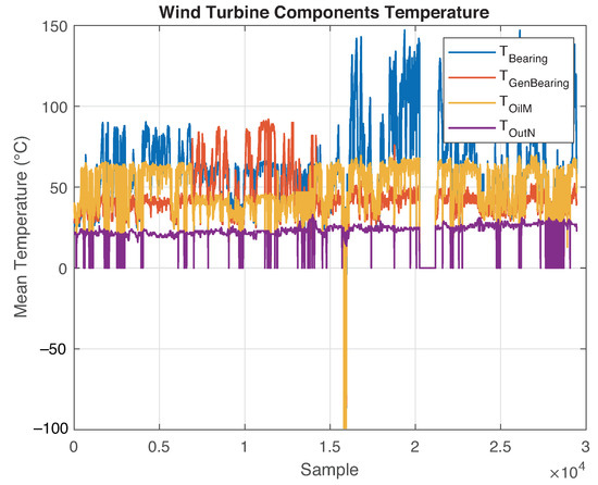
Figure 1.
Temperature variables plot: denotes the WT main bearing temperature, corresponds to the temperature of the generator bearing, represents the oil temperature inside the gearbox, and represents the nacelle temperature.
The complete period of faulty observations can be identified after comparing the date and time of each alarm log from the alarm report with the date and time of the monitoring data. Thus, all data between the ON and OFF states are considered faulty. This process adds a vector of labels to the dataset, wherein 1 indicates that an observation is classified as faulty, and 0 indicates a healthy observation. For visualization, and considering that the alarms are related to the gearbox temperature, faulty observations were plotted along with the oil temperature variables, as shown in Figure 2 and Figure 3.
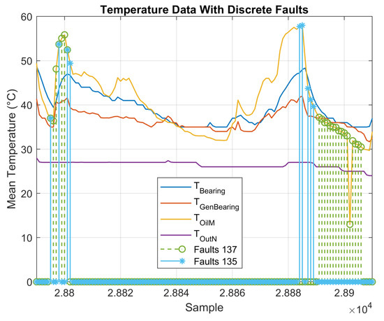
Figure 2.
Measured temperatures and associated discrete faults.
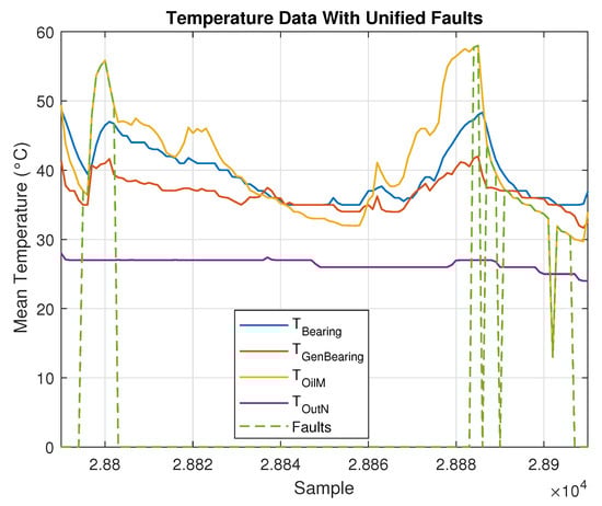
Figure 3.
Measured temperatures and associated merged faults.
3.2. Data Modeling and Dimension Reduction by Principal Component Analysis
After the initial stage of data integration that includes data imputation and labeling, PCA was used for both data transformation and data reduction. In the present framework, data transformation is understood as the application of a particular function to each element in the dataset to uncover hidden patterns. Data reduction is conducted to reduce data complexity and computational effort and time. The PCA transforms the dataset into a new set of uncorrelated variables called principal components (PCs) that are sorted in the descending order with respect to the retained variance given by the eigenvalues of the variance–covariance matrix [34].
The algorithm of the proposed approach is described as follows. Consider the initial dataset
where and .
Matrix D comprises a matrix , which contains N observations (or samples) described by p features (or variables) called , and a vector that contains N known labels of healthy (0) and faulty data (1).
When the following set is defined
data in matrix D in Equation (1) are split into healthy data (H) and faulty data (F)
where and are the total number of healthy and faulty observations, respectively.
Then, healthy data are standardized using Z-score normalization. The standard deviation of each column is equal to 1, and its mean is equal to 0. This is calculated as
where represents the element in the ith row and the jth column of matrix H. The standardized healthy data are now called . Then, the variance–covariance matrix of is computed as
where denotes the number of observations (rows) in matrix .
The PCA identifies linear manifolds characterizing the data by diagonalizing the variance–covariance matrix , where the diagonal terms of are
Analogously, the eigenvectors that form the columns of matrix P are sorted in the same order. The matrix is called the PCA model of the dataset H, where each column of this matrix corresponds to a linear combination of the features of the normalized healthy dataset .
In the next step, the faulty data stored in F are standardized using the mean and standard deviation of the corresponding column of healthy data
where denotes the element in the ith row and jth column of matrix F.
Finally, all data are transformed using the PCA model P as
The transformed datasets and are the projections of the normalized healthy () and faulty () datasets onto the vector space spanned by the PCs. This process is applied to the training and testing datasets of the ML algorithms.
For a comprehensive study of these datasets and the effect of the PCA model, the proportion of variance explained (PVE) or explained variation is used. The PVE measures the proportion at which a mathematical model affects the dispersion of a dataset. The PCA is used to analyze the distribution of information among the PCs to select components that can be discarded. Several tools have been proposed to study the explained variations. For example, the scree plot is a graphical tool built by plotting the individual explained variances of each PC along with the cumulative PVE (CPVE) obtained by adding the PVE of each PC individually. The PVE associated with the jth principal component is
while the CPVE of the first j PCs is
The scree plot of the PCA model is shown in Figure 4.
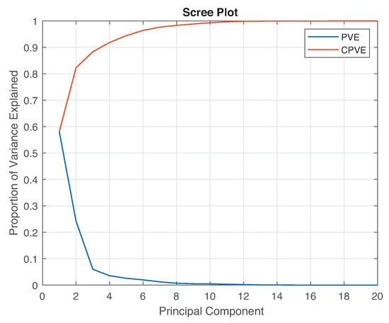
Figure 4.
Principal components analysis scree plot.
Figure 4 shows the distribution of variance among the different PCs, which indicates where the most information is located. Therefore, the transformation using only PCs induces a change because a reduced version of the PCA model is used as
Dimensionality reduction is performed using the reduced PCA model defined in Equation (9):
According to Figure 4, the first PCs are the most suitable for use as they account for over of the cumulative variance.
To observe the distribution of the faults and healthy data, the first three PCs are plotted, as shown in Figure 5. Figure 5 shows the large difference between the number of the members of each class (healthy and faulty). This is a highly imbalanced dataset containing 29,459 healthy observations and only 29 faults—a condition that can lead to a bias toward the healthy class when using the dataset to train an ML algorithm.
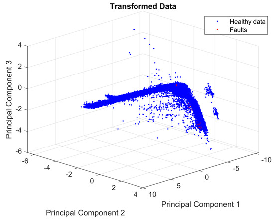
Figure 5.
Projection of normalized data into the vector space spanned by the first three principal components.
3.3. Techniques for Dealing with Imbalanced Data
Two balancing techniques are proposed to deal with the highly imbalanced dataset: the first is random oversampling, which is a simple and effective technique used to generate random synthetic data from the minority class of the dataset. This technique can outperform the undersampling technique [35] when used to enhance classification processes [36]. Furthermore, this technique can be combined with advanced preprocessing techniques [37] to obtain better results.
The second technique is a data augmentation method based on data reshaping. Data augmentation works by increasing the number of available samples without increasing the size of the dataset. It is frequently used to enhance deep learning algorithms that use images [38,39]. The performance of these algorithms depends on the shape and distribution of the input data. Thus, different reshaping techniques have been developed to improve their effectiveness [40]. Studies have been performed on reshaping time-series data. For example, acoustic signals have been reshaped as a matrix by following the same principles used by deep learning algorithms with images [41], whereas multisensory time series data have been reshaped for tool wear prediction [42]. A data-reshaping technique for time series data was proposed based on these ideas. This technique is similar to the one used with acoustic signals, which encapsulates the time series by creating a new matrix for each time window to add more information to each observation without increasing the size of the dataset. Several time window shapes are proposed to determine their effect on each classification algorithm, and the most appropriate one for SCADA data are selected. This technique can be used with the random oversampling technique if the data remain imbalanced after processing. These techniques are described in detail below.
3.3.1. Random Oversampling
The random oversampling technique is widely used to solve the imbalanced data problem because of its simplicity and effectiveness. It is a non-heuristic method that replicates the observations of determinate characteristics from the minority class to balance the dataset [43]. However, despite its simplicity, it must be used carefully because it can lead to overfitting of ML algorithms [44].
The technique generates synthetic observations from each observation of the minority class by adding random Gaussian noise. This produces a vector of observations. The natural number n can be calculated using the ratio of the size of each class to balance them and obtain a proportion in the case of a binary classification. Furthermore, it can be selected arbitrarily based on the requirements of the study. Equations (12) and (13) describe the oversampling approach as
where represents the realization of the random variable . As stated in Equations (12) and (13), a standard Gaussian random noise is added to each observation with a linear scale factor of . When introducing synthetic observations, if the dataset is time-dependent, such as SCADA data, the time-dependence must not be altered. The synthetic observations must be inserted immediately after they are generated by the original observation to avoid altering this time-dependence.
In the initial test, was used. This selection allows the generation of a vector with 29,000 synthetic faults, and it also includes the original faults, as described previously. Figure 6 shows the distribution of the transformed data with fault oversampling.
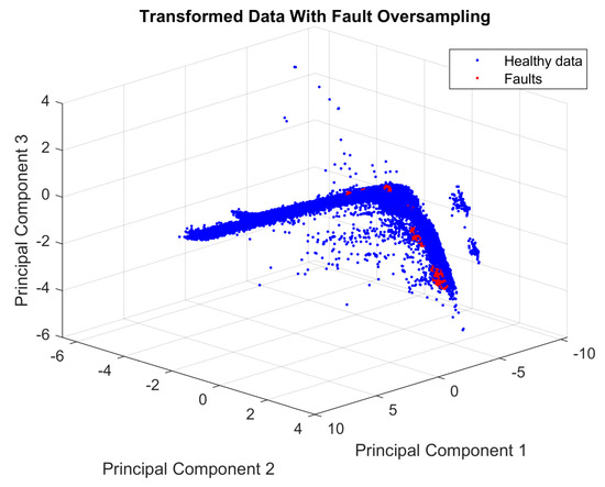
Figure 6.
Projection of normalized data into the vector space spanned by the first three principal components and the oversampled faulty data.
3.3.2. Data Reshaping
In the initial dataset described in Equation (1), we have N observations (or samples) described by p features (or variables). To enhance the quality of information provided by each sample, we propose data reshaping, which is a data processing technique that helps the classifier extract as much information as possible from the studied event. The method comprises four steps, and it is illustrated in Figure 7 using the distribution of one of the variables of the dataset and its time-dependence.
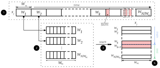
Figure 7.
Graphical description of the data reshaping technique.
- Step 1. Each feature of the dataset described in Equation (1) is divided into small pieces of data called windows , where represents the floor function. All windows must contain the same number of observations. The number of observations captured by each window is called the window size , which determines the amount of data captured. Therefore, it must be selected carefully; if a large amount of data are captured, then important patterns of the dataset may be removed when these are grouped over a single new sample. In contrast, if insufficient data are captured, then the method will be ineffective because the new sample will not be sufficiently rich to enhance the process. To avoid these drawbacks, was carefully selected by considering the characteristics of the dataset such as sampling time, amount of data, and physical variable behavior. All data are collected such that, if the dataset is time-dependent, it will not mix any observations to maintain its time-dependence and avoid data leakage.
- Step 2. All information inside the window , of size is captured and stored as a new observation. All windows that contain at least one faulty observation are relabeled as faulty.
- Step 3. Each new observation is stacked to create a new feature matrix with dimensions .
- Step 4. After reshaping the data, it can be split into training and testing sets to be standardized and used to train and test the models.
3.4. Machine Learning Classifiers
The ML algorithms selected to detect faults in WTs are two classical methods: kNN and SVM. These two methods were compared with RUSBoost, which was designed to deal with the imbalanced data problem. It is known for its excellent performance. In the context of the present work, RUSBoost was used as the baseline to test the proposed data preprocessing techniques, and it was applied with the classical methods to deal with the imbalanced data problem.
3.4.1. k Nearest Neighbors (kNN)
kNN is one of the simplest ML algorithms [45]. Given a new data point to be classified, this algorithm finds the closest k data points in the set, i.e., the so-called nearest neighbors. The new data point is then classified based on multiple votes of the neighbors (majority vote in the case of binary classification). This means that the studied point is classified into the same class as the majority of its neighbors (see Figure 8a). The words nearest or closest imply the measurement of the distance between the studied sample and its neighbors; measuring this distance may lead to variations in this approach. The most common is the Euclidean distance, which is a special case of the Minkowski distance, i.e., the Minkowski distance of order 2 [46].
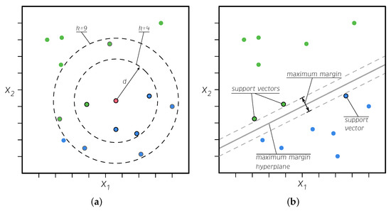
Figure 8.
Graphical description of the kNN (a) and SVM (b) algorithms.
3.4.2. Support Vector Machines (SVM)
An SVM is a powerful ML algorithm that can perform linear and nonlinear classification and regression, and it is well suited for complex, medium, or small datasets [47]. This method, which is also called the maximum margin classifier, finds the widest gap between classes. The data points that exceed the limits of the margin near the separator are called support vectors as they hold up the separator (see Figure 8b). The kernel trick—a function called a kernel is used to transform the data into a higher dimension to make it more separable—is used to extrapolate this method to higher dimensions and more complex data. The SVM combines the advantages of the nonparametric and parametric models, which have the flexibility to represent complex functions but are resistant to overfitting [46].
3.4.3. Random under Sampling Boost (RUSBoost)
RUSBoost belongs to the family of ensemble methods of ML, specifically those that use hypothesis boosting. The boosting refers to any ensemble method that combines several weak learners (other common ML algorithms) into a strong learner. The general idea of most boosting methods is to train predictors sequentially and iteratively to improve their predecessor [47]. This algorithm was specifically designed to work with imbalanced datasets using undersampling. This involves taking N, the number of members in the class with the least members in the training data, and taking only N observations of every other class with more members in it. That is, if there are K classes, then, for each weak learner in the ensemble, RUSBoost takes a subset of the data with N observations from each of the K classes [48].
3.4.4. Performance Measures for Machine Learning Classifiers
Several indicators have been developed to measure the performance of ML algorithms. These indicators are based on the capacity of the algorithm to classify the different objects presented to them. The metrics calculation process uses a block of the dataset to train the ML model (training data), and then the model is used to classify the remaining data (testing data). This process generates a set of predicted labels that are compared with the original data labels. The overall process is called supervised learning, and it can be used for binary classification (two labels in the data) or multiclass classification (more than two labels) [49]. The former is used in the present study. The comparison of real and predicted labels enables the creation of a confusion matrix, as shown in Table 4.
Table 4.
Confusion matrix for binary classification performance assessment.
In Table 4, denotes the number of observations classified as positive, and denotes the number of observations that are classified as positive but are truly negative. Similarly, represents the number of observations classified as negative, and represents the number of observations that are classified as negative but are truly positive. All confusion matrices in this study contain the information listed in Table 4 with a few additions for improved analysis. The performance measures can be calculated as shown in Equations (14)–(21).
- Accuracy (). Measures the number of correct predictions made by the model over the total number of observations.
- Precision or positive predictive value (). Measures the number of correctly classified positive class labels over the total number of positive-predicted labels, and it describes the proportion of correctly predicted positive observations.
- False discovery rate (). Measures the number of incorrectly classified positive class labels over the total number of positive predicted labels, describes the proportion of incorrectly predicted positive observations, and complements the information obtained by the precision.
- Negative predictive value (). Measures the number of correctly classified negative-class labels over the total number of negative predicted labels, and it describes the proportion of correctly predicted negative observations.
- False omission rate (). Measures the number of incorrectly classified negative-class labels over the total number of negative predicted labels, describes the proportion of incorrectly predicted negative observations, and it is complementary to the negative predictive value.
- Sensitivity/Recall/True positive rate (). Describes the fraction of correctly classified positive observations.
- F1 score (). It is the harmonic mean between precision and recall. It is calculated using
- Specificity/False positive rate (). The harmonic mean between precision and recall.
3.5. Experimental Framework
Two tests were conducted to select the best fault detection method. A flowchart of the proposed approach and how it is applied is given in Figure 9. The tests are defined as follows:
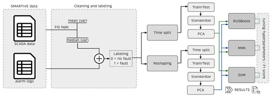
Figure 9.
Flowchart of the proposed approach. SCADA data are first cleaned and labeled and then processed using two strategies: time split and reshaping. After, rescaled and projected into the PCA model before the ML classifiers. ML classifiers are tuned using the Score to get the best possible results.
- Test 1. The dataset was split at an observation labeled as faulty. That observation was strategically selected to ensure that the resulting subsets have sufficient healthy and faulty information for the training and testing processes. Another reason to split the dataset this way is to maintain its time-dependence and eliminate the risk of data leakage. Therefore, this approach is called the time split. Afterwards, the data are standardized and modeled with the PCA method. The RUSBoost algorithm was fed with these data without any further processing to create a performance baseline. Then, the training and testing datasets used to feed the kNN and SVM algorithms were oversampled to create a balance using or , depending on which one is the minority class. This method is illustrated in Figure 10.
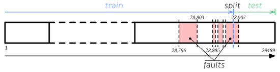 Figure 10. Graphical description of the time split method using the distribution of the used data set.
 - Test 2. The time series dataset was reshaped as detailed in Section 3.3.2. The new observations with faults were identified, and the observations were modeled using the PCA method. Then, the data were split using the method described in test 1 (time split). The RUSBoost algorithm was fed with reshaped data without any further processing to obtain the performance baseline. The training and testing datasets used to feed the kNN and SVM algorithms were oversampled; the oversampling method became necessary as the data imbalance was worsened by reshaping. The balance is generated using or , depending on which is the minority class.
For all tests, the ML algorithms were tuned by predicting the labels using the testing dataset. Using these labels, the performance metrics were calculated and stored at each iteration of the grid search algorithm. This algorithm sweeps over various previously defined hyperparameters, and it selects the best one using the highest score obtained from all performed tests. The score was considered because it reduces false positives and false negatives by creating a trade-off between precision and recall; simultaneously, it improves the detection of true positives.
The hyperparameters selected to tune each algorithm are
- k-nearest neighbors. In this algorithm, the number of nearest neighbors swept is between 1 and 200, and the Euclidean distance is used.
- SVM. The SVM is configured to function as a nonlinear separator using the radial basis function. It is tuned using the kernel scale (commonly known as the gamma factor) and a box constraint C (also known as the C factor or weighting factor) for the misclassified data. To test soft and hard classification boundaries, the hyperparameters were changed from small to large values. The number of PCs () selected for each dataset was considered to tune the kernel scale. Furthermore, the kernel scale was computed as the weighted square root of the number of PCs of the dataset used.
- RUSBoost. The hyperparameters of this algorithm are the maximum splits of the tree , the number of learning cycles , or iterations where the algorithm is going to run to select the best tree by majority voting. The learning rate that controls the shrinkage of the contribution of each new base model added to the series via gradient boosting is
4. Results
Non-oversampled and oversampled datasets were split and transformed according to the tests described in the previous section. The resulting data distributions are summarized in Table 5 and Table 6. In both tables, Obs denotes the number of observations.
Table 5.
Non-oversampled dataset characteristics after applying the splitting techniques per test.
Table 6.
Oversampled data set characteristics after applying the splitting techniques per test.
4.1. Test 1: Time Split
4.1.1. kNN Results
The optimal hyperparameters that yield the best possible classification results using the kNN algorithm are and nearest neighbors for the non-oversampled and oversampled data, respectively. The confusion matrices for the aforementioned cases are shown in Figure 11.
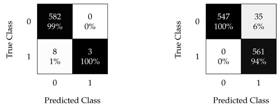
Figure 11.
kNN confusion matrix using non-oversampled (left) and oversampled (right) data with the time split (test 1).
Figure 11 demonstrates the effectiveness of the oversampling method technique when time-splitting the data to train the kNN model. Time-splitting enables the detection of all faults with only a false discovery rate when oversampling.
4.1.2. SVM Results
The optimal hyperparameters that yield the best possible classification results using the SVM algorithm are listed in Table 7.
Table 7.
Optimal hyperparameters for the SVM in test 1.
Figure 12 shows the confusion matrices for the SVM algorithm, where the oversampling technique with time splitting is very effective. Furthermore, it allows the classification of most faults with an of and of for the oversampled and non-oversampled cases, respectively. This implies that the kNN algorithm achieves a slightly better performance for this type of analysis.
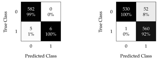
Figure 12.
SVM confusion matrix using non-oversampled (left) and oversampled (right) data with the time split (test 1).
4.1.3. RUSBoost Results
Table 8 lists the optimal hyperparameters obtained for the RUSBoost algorithm.
Table 8.
Optimal hyperparameters for the RUSBoost in test 1.
Figure 13 shows the RUSBoost results with the optimal hyperparameters to be used as the baseline. Recall that this algorithm was specifically designed to handle highly imbalanced datasets. In this specific dataset, all faulty samples can be correctly classified, but with an of . These results demonstrate the effectiveness of the oversampling technique compared with the undersampling method used by the RUSBoost algorithm for this type of dataset. Oversampling empowers the kNN method to perform better than the RUSBoost algorithm on the same initial dataset.
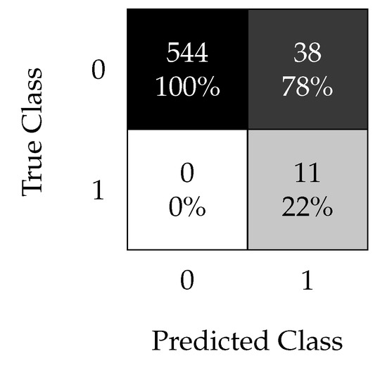
Figure 13.
RUSBoost confusion matrix using the non-oversampled data set with the time split (test 1).
4.1.4. Performance Charts
The performance charts (Table 9) summarize the performance metrics calculated for each algorithm with the time-split data division. Recall that the hyperparameters of the algorithms were tuned by optimizing the score.
Table 9.
Performance metrics comparison for results obtained with the time split (test 1).
Table 9 highlights the effect of the oversampling technique combined with the time split for the time-dependent data.
RUSBoost achieved a sensitivity of ; however, it achieved a precision of only . As expected, the non-oversampling strategies with kNN and SVM exhibited poor performance with low sensitivities of and , respectively; the oversampling strategies achieved high sensitivity and precision scores exceeding in both cases.
Table 10 lists the training and prediction times for a single sample using each algorithm on a laptop with 12 GB RAM, and an i7 processor running on a Microsoft Windows home operating system, version 20H2. The table highlights another advantage of using the oversampling technique, i.e., the training and prediction times of the algorithms fed with oversampled data that are considerably lower than those of the RUSBoost method.
Table 10.
Computation time per algorithm while training and predicting one single sample using time split (test 1).
4.2. Test 2: Data Reshaping
4.2.1. kNN Results
The optimal hyperparameters that yield the best model using the kNN algorithm are listed in Table 11 for each time window considered.
Table 11.
Optimal hyperparameter for kNN in test 2.
Figure 14 shows the confusion matrices obtained for the different reshaping window sizes considered.
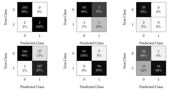
Figure 14.
kNN confusion matrices. Results without oversampling (top) and with oversampled data (bottom); results with a time windows of 30 min (left), 1 h (center), and 3 h (right).
The first row of plots in Figure 14 are related to the non-oversampled data, where the imbalanced dataset clearly leads to poor sensitivity for all time windows (all or half of the faulty samples were not detected). Figure 14 (left) shows the results obtained by feeding the kNN algorithm with the reshaped modeled data with a time window of 30 min with and without oversampling. Using the oversampling technique significantly improved the performance. Figure 14 (center) shows the results obtained using a time window of 1 h. In the non-oversampled case, the performance decreased with an and of and , respectively, in contrast with the performance of the 30 min window. The oversampled case obtained the best results; it reached an of with an of compared with the previously shown time window. Finally, Figure 14 (right) shows the results obtained with the 3 h time window, which were worse than the previous time reshapes.
4.2.2. SVM Results
The optimal hyperparameters that yield the best possible classification results using the SVM algorithm are listed in Table 12.
Table 12.
Optimal hyperparameters for SVM in test 2.
Figure 15 shows the confusion matrices calculated using the predicted labels.
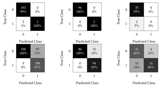
Figure 15.
SVM confusion matrices. Results without oversampling (top) and with oversampled data (bottom); results with a time window of 6 h (left), 12 h (middle), and 24 h (right).
Figure 15 (left) shows the results obtained by feeding the SVM algorithm with the reshaped modeled data with a time window of 30 min. As expected, the oversampling dramatically improved the results. Figure 15 (center) shows the results obtained using a time window of 1 h. It was observed that reshaping can enhance the classification process using the SVM when trained with imbalanced data because it leads to the correct classification of a pair of faulty samples among 98 observations with non-oversampled data. Furthermore, oversampled data achieve good performance, showing an of only and the perfect classification of healthy data. Figure 15 (right) shows the results obtained using a time window of 3 h. This is the same as that for the kNN; the worst results were obtained with this time window.
4.2.3. RUSBoost Results
The optimal hyperparameters that yield the best classifier using the RUSBoost algorithm are listed in Table 13.
Table 13.
Optimal hyperparameter for RUSBoost in test 2.
Figure 16 shows the confusion matrices calculated using the predicted labels.
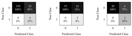
Figure 16.
RUSBoost confusion matrix using data processed with a time window of 30 min (left), 1 h (center), and 3 h (right).
Figure 16 shows the results of feeding the RUSBoost algorithm with reshaped data using time windows of 30 min (left), 1 h (center), and 3 h (right), respectively. In all cases, the RUSBoost algorithm achieved a high sensitivity () but with low precision; i.e., it generated a significant number of false positives that produce of for the best case (3 h window) and for the worst case (1 h window).
4.2.4. Performance Charts
Table 14 and Table 15 show the performance and execution times of the algorithms fed with the reshaped and oversampled data.
Table 14.
Performance metrics comparison (test 2) when using time windows of 0.5, 1, and 3 h.
Table 15.
Computation time per algorithm (test 2) while training and predicting one single sample using processed data with time windows of 0.5, 1, and 3 h.
Table 14 summarizes the performance of the proposed algorithms. First, it shows that the performance of the 30 min time window is acceptable for both kNN and SVM; however, it is poor for RUSBoost, where it achieves a precision of only . The score always improves when using the oversampling technique for kNN and SVM. Second, the performance was further improved using the 1 h time window compared with the 30 min window, which makes it the best candidate for this application. For the 1 h time window, the performance of RUSBoost was unacceptable, with a precision of only . Finally, even when oversampling the data, the 3 h time window led to the poor performance of the SVM and RUSBoost algorithms. The kNN algorithm achieved a precision of with oversampled data; however, it had a recall of .
In terms of execution time, as summarized in Table 15, the main disadvantage of the ensemble methods (e.g., RUSBoost algorithm) is the heavy computational burden; hence, they are slower than other algorithms (even when other methods use reshaped and oversampled data). The RUSBoost algorithm has a high degree of variability in terms of execution time. For example, with time windows of 30 min, 1 h, and 3 h, the training times are s, s, and s, respectively.
For the other algorithms, the execution times were consistent even when the number of features increased because of the use of the reshaping technique.
5. Discussion
All tests showed that the classification process can be significantly enhanced by properly preprocessing the data.
In this study, the first preprocessing technique was PCA, and it was used to generate a normal (healthy) model to project the faulty data using the same model. This approach makes the faulty data more separable while significantly reducing the amount of data required to obtain good performance classification results. Furthermore, another advantage of PCA is that the training and prediction times are reduced because of the feature reduction.
The second proposed preprocessing technique is random oversampling, which is proven to be a simple yet efficient solution to deal with imbalanced data. With oversampling, the resulting metrics improved significantly, thereby enabling competition and surpassing the effectiveness of the baseline algorithm RUSBoost. Furthermore, oversampling on the highly imbalanced dataset presented in this study improved the training and prediction execution times with respect to the baseline. When combined with the time-split technique, oversampling significantly improves the effectiveness of the models. Finally, the proposed data reshaping technique has a performance that is similar to that of a simple time-split because of a major drawback of the specific available dataset, i.e., faulty data were concentrated over a small time-frame at the end of the dataset. Thus, there are limitations to splitting the data between the training and testing sets, and reshaping by itself cannot balance the dataset. However, if fault observations are separated with longer time intervals, the reshaping can improve the imbalanced data problem. In addition, when using reshaping, training and prediction times increased because of the expanded set of features per sample. The tests performed identified the 1 h time window as the best for this application.
6. Conclusions
Artificial intelligence is an exponentially growing field that is of great importance in many fields of research. In the WT industry, it is a promising tool to optimize the maintenance process as it can enable the early prediction of faults which can help ensure energy production throughout the year. In this study, three data preprocessing strategies were tested to enhance the fault detection process when using a highly imbalanced dataset. These strategies are PCA for data modeling and reduction; a random oversampling technique to deal with the imbalanced data problem; and the data reshaping technique for data augmentation to increase the amount of information per sample. A time split was used to avoid corrupting the time structure of the dataset (when the data are time-dependent) and to prevent data leakage when training the ML algorithms. The combination of these data preprocessing techniques leads to the excellent performance of classification algorithms. The results surpassed those obtained with RUSBoost to deal with data imbalance. Furthermore, the results showed scores of at least , thereby fulfilling one of the main objectives of the study. The random oversampling technique improved all results, and it can be tuned for a specific dataset using a variable scaling factor. Even when the reshaping technique performance was weaker than expected, it had a great potential. It enriched the information contained in each observation; for example, it enabled algorithms to classify a single faulty observation among a pool of healthy ones. Furthermore, it is important to note that the window size must be carefully selected depending on the nature of the data because it can cause a considerable difference in capturing data patterns or trends.
The feasible practical application of the proposed methodology is noteworthy. First, the required SCADA data are available in all industrial sized wind turbines. Second, but directly related to the previous point, no extra equipment is needed to be installed, thus the methodology is cost-effective as it has a very low deployment cost. Third, the computational complexity (computational time and required storage) to estimate new predictions is low and can be done on real-time at each wind turbine (on-site) or at the wind park data center. Finally, the stated strategy works under all regions of operation of the wind turbine (below the rated wind speed, and above the rated wind speed), thus the wind turbine is always under supervision.
In the future work, the proposed techniques should be implemented using a larger dataset containing more error frames (distributed and separated between them in time) to be detected, which will allow a more comprehensive testing of the effectiveness of the reshaping technique.
Author Contributions
All authors contributed equally to this work. All authors have read and agreed to the published version of the manuscript.
Funding
This work was partially funded by the Spanish Agencia Estatal de Investigación (AEI)—Ministerio de Economía, Industria y Competitividad (MINECO), and the Fondo Europeo de Desarrollo Regional (FEDER) through the research project DPI2017-82930-C2-1-R; and by the Generalitat de Catalunya through the research project 2017 SGR 388. We gratefully acknowledge the support of NVIDIA Corporation with the donation of the Titan Xp GPU used for this research.
Institutional Review Board Statement
Not applicable.
Informed Consent Statement
Not applicable.
Data Availability Statement
The data required to reproduce these findings cannot be shared at this time as it is proprietary.
Acknowledgments
The authors express their gratitude and appreciation to the Smartive company (http://smartive.eu/ (accessed on 18 March 2021)); this work would not have been possible without their support and wind farm data.
Conflicts of Interest
The authors declare no conflict of interest.
Abbreviations
The following abbreviations are used in the manuscript:
| Accuracy | |
| CPVE | Cumulative proportion of variance explained |
| score | |
| False discovery rate | |
| False negative | |
| False omission rate | |
| False positive | |
| False positive rate | |
| kNN | k-nearest neighbors |
| Negative predictive value | |
| Obs | Observations |
| OS | Operating system |
| PC | Principal component |
| PCA | Principal component analysis |
| Positive predictive value | |
| PVE | Proportion of variance explained |
| RUSBoost | Random under sampling boost |
| SCADA | Supervisory control and data acquisition |
| SVM | Support vector machine |
| True negative | |
| True positive | |
| True positive rate | |
| WT | Wind turbine |
References
- Wang, S.; Yang, H.; Pham, Q.B.; Khoi, D.N.; Nhi, P.T.T. An Ensemble Framework to Investigate Wind Energy Sustainability Considering Climate Change Impacts. Sustainability 2020, 12, 876. [Google Scholar] [CrossRef]
- Rosales-Asensio, E.; Borge-Diez, D.; Blanes-Peiró, J.J.; Pérez-Hoyos, A.; Comenar-Santos, A. Review of wind energy technology and associated market and economic conditions in Spain. Renew. Sustain. Energy Rev. 2019, 101, 415–427. [Google Scholar] [CrossRef]
- Wind Energy in Spain. Available online: https://www.aeeolica.org/en/about-wind-energy/wind-energy-in-spain/ (accessed on 1 February 2021).
- Rodríguez, X.A.; Regueiro, R.M.; Doldán, X.R. Analysis of productivity in the Spanish wind industry. Renew. Sustain. Energy Rev. 2020, 118, 109573. [Google Scholar] [CrossRef]
- Spain Hits 44.7% Renewables Share in 7-mo 2020. Available online: https://renewablesnow.com/news/spain-hits-447-renewables-share-in-7-mo-2020-708939/ (accessed on 3 February 2021).
- Shafiee, M.; Sørensen, J.D. Maintenance optimization and inspection planning of wind energy assets: Models, methods and strategies. Reliab. Eng. Syst. Saf. 2019, 192, 105993. [Google Scholar] [CrossRef]
- Lin, J.; Pulido, J.; Asplund, M. Reliability analysis for preventive maintenance based on classical and Bayesian semi-parametric degradation approaches using locomotive wheel-sets as a case study. Reliab. Eng. Syst. Saf. 2015, 134, 143–156. [Google Scholar] [CrossRef]
- Florescu, A.; Barabas, S.; Dobrescu, T. Research on Increasing the Performance of Wind Power Plants for Sustainable Development. Sustainability 2019, 11, 1266. [Google Scholar] [CrossRef]
- Krishna, D.G. Preventive maintenance of wind turbines using Remote Instrument Monitoring System. In Proceedings of the 2012 IEEE Fifth Power India Conference, Murthal, India, 19–22 December 2012; pp. 1–4. [Google Scholar]
- Mazidi, P.; Du, M.; Tjernberg, L.B.; Bobi, M.A.S. A performance and maintenance evaluation framework for wind turbines. In Proceedings of the 2016 International Conference on Probabilistic Methods Applied to Power Systems (PMAPS), Beijing, China, 16–20 October 2016; pp. 1–8. [Google Scholar]
- Sequeira, C.; Pacheco, A.; Galego, P.; Gorbeña, E. Analysis of the efficiency of wind turbine gearboxes using the temperature variable. Renew. Energy 2019, 135, 465–472. [Google Scholar] [CrossRef]
- Lebranchu, A.; Charbonnier, S.; Bérenguer, C.; Prévost, F. A combined mono- and multi-turbine approach for fault indicator synthesis and wind turbine monitoring using SCADA data. ISA Trans. 2019, 87, 272–281. [Google Scholar] [CrossRef]
- Wang, K.S.; Sharma, V.S.; Zhang, Z.Y. SCADA data based condition monitoring of wind turbines. Adv. Manuf. 2014, 2, 61–69. [Google Scholar] [CrossRef]
- Kusiak, A.; Verma, A. Analyzing bearing faults in wind turbines: A data-mining approach. Renew. Energy 2012, 48, 110–116. [Google Scholar] [CrossRef]
- Dao, P.B.; Staszewski, W.J.; Barszcz, T.; Uhl, T. Condition monitoring and fault detection in wind turbines based on cointegration analysis of SCADA data. Renew. Energy 2018, 116, 107–122. [Google Scholar] [CrossRef]
- Alvarez, E.J.; Ribaric, A.P. An improved-accuracy method for fatigue load analysis of wind turbine gearbox based on SCADA. Renew. Energy 2018, 115, 391–399. [Google Scholar] [CrossRef]
- Rodríguez-López, M.A.; López-González, L.M.; López-Ochoa, L.M.; Las-Heras-Casas, J. Development of indicators for the detection of equipment malfunctions and degradation estimation based on digital signals (alarms and events) from operation SCADA. Renew. Energy 2016, 99, 224–236. [Google Scholar] [CrossRef]
- Qiu, Y.; Feng, Y.; Infield, D. Fault diagnosis of wind turbine with SCADA alarms based multidimensional information processing method. Renew. Energy 2020, 145, 1923–1931. [Google Scholar] [CrossRef]
- Dai, J.; Yang, W.; Cao, J.; Liu, D.; Long, X. Ageing assessment of a wind turbine over time by interpreting wind farm SCADA data. Renew. Energy 2018, 116, 199–208. [Google Scholar] [CrossRef]
- Ruiming, F.; Minling, W.; Xinhua, G.; Rongyan, S.; Pengfei, S. Identifying early defects of wind turbine based on SCADA data and dynamical network marker. Renew. Energy 2020, 154, 625–635. [Google Scholar] [CrossRef]
- Jha, S.K.; Bilalovic, J.; Jha, A.; Patel, N.; Zhang, H. Renewable energy: Present research and future scope of Artificial Intelligence. Renew. Sustain. Energy Rev. 2017, 77, 297–317. [Google Scholar] [CrossRef]
- Pozo, F.; Vidal, Y.; Serrahima, J.M. On real-time fault detection in wind turbines: Sensor selection algorithm and detection time reduction analysis. Energies 2016, 9, 520. [Google Scholar] [CrossRef]
- Bangalore, P.; Patriksson, M. Analysis of SCADA data for early fault detection, with application to the maintenance management of wind turbines. Renew. Energy 2018, 115, 521–532. [Google Scholar] [CrossRef]
- Zhao, H.; Liu, H.; Hu, W.; Yan, X. Anomaly detection and fault analysis of wind turbine components based on deep learning network. Renew. Energy 2018, 127, 825–834. [Google Scholar] [CrossRef]
- Kong, Z.; Tang, B.; Deng, L.; Liu, W.; Han, Y. Condition monitoring of wind turbines based on spatio-temporal fusion of SCADA data by convolutional neural networks and gated recurrent units. Renew. Energy 2020, 146, 760–768. [Google Scholar] [CrossRef]
- Helbing, G.; Ritter, M. Deep Learning for fault detection in wind turbines. Renew. Sustain. Energy Rev. 2018, 98, 189–198. [Google Scholar] [CrossRef]
- Imbalanced Data. Available online: https://developers.google.com/machine-learning/data-prep/construct/sampling-splitting/imbalanced-data (accessed on 11 March 2021).
- Castellani, F.; Garibaldi, L.; Daga, A.P.; Astolfi, D.; Natili, F. Diagnosis of faulty wind turbine bearings using tower vibration measurements. Energies 2020, 13, 1474. [Google Scholar] [CrossRef]
- Wang, Y.; Ma, X.; Qian, P. Wind turbine fault detection and identification through PCA-based optimal variable selection. IEEE Trans. Sustain. Energy 2018, 9, 1627–1635. [Google Scholar] [CrossRef]
- Zhao, Y.; Li, D.; Dong, A.; Kang, D.; Lv, Q.; Shang, L. Fault prediction and diagnosis of wind turbine generators using SCADA data. Energies 2017, 10, 1210. [Google Scholar] [CrossRef]
- Pozo, F.; Vidal, Y. Wind turbine fault detection through principal component analysis and statistical hypothesis testing. Energies 2016, 9, 3. [Google Scholar] [CrossRef]
- Pozo, F.; Vidal, Y.; Salgado, Ó. Wind turbine condition monitoring strategy through multiway PCA and multivariate inference. Energies 2018, 11, 749. [Google Scholar] [CrossRef]
- Fleckestein, J.E. Three-Phase Electrical Power; CRC Press: Boca Raton, FL, USA, 2016. [Google Scholar]
- Jolliffe, I.T. Principal Component Analysis; Springer: Berlin/Heidelberg, Germany, 2002. [Google Scholar]
- Mohammed, R.; Rawashdeh, J.; Abdullah, M. Machine Learning with Oversampling and Undersampling Techniques: Overview Study and Experimental Results. In Proceedings of the 2020 11th International Conference on Information and Communication Systems (ICICS), Irbid, Jordan, 7–9 April 2020; pp. 243–248. [Google Scholar]
- Pang, Y.; Chen, Z.; Peng, L.; Ma, K.; Zhao, C.; Ji, K. A Signature-Based Assistant Random Oversampling Method for Malware Detection. In Proceedings of the 2019 18th IEEE International Conference On Trust, Security and Privacy in Computing and Communications/13th IEEE International Conference on Big Data Science and Engineering (TrustCom/BigDataSE), Rotorua, New Zealand, 5–8 August 2019; pp. 256–263. [Google Scholar]
- Ghazikhani, A.; Yazdi, H.S.; Monsefi, R. Class imbalance handling using wrapper-based random oversampling. In Proceedings of the 20th Iranian Conference on Electrical Engineering (ICEE2012), Tehran, Iran, 15–17 May 2012; pp. 611–616. [Google Scholar]
- Puruncajas, B.; Vidal, Y.; Tutivén, C. Vibration-Response-Only Structural Health Monitoring for Offshore Wind Turbine Jacket Foundations via Convolutional Neural Networks. Sensors 2020, 20, 3429. [Google Scholar] [CrossRef] [PubMed]
- Ruiz, M.; Mujica, L.E.; Alferez, S.; Acho, L.; Tutiven, C.; Vidal, Y.; Rodellar, J.; Pozo, F. Wind turbine fault detection and classification by means of image texture analysis. Mech. Syst. Signal Process. 2018, 107, 149–167. [Google Scholar] [CrossRef]
- Ghosh, S.; Das, N.; Nasipuri, M. Reshaping inputs for convolutional neural network: Some common and uncommon methods. Pattern Recognit. 2019, 93, 79–94. [Google Scholar] [CrossRef]
- Janssen, L.A.L.; Lopez Arteaga, I. Data processing and augmentation of acoustic array signals for fault detection with machine learning. J. Sound Vib. 2020, 483, 115483. [Google Scholar] [CrossRef]
- Huang, Z.; Zhu, J.; Lei, J.; Li, X.; Tian, F. Tool Wear Predicting Based on Multisensory Raw Signals Fusion by Reshaped Time Series Convolutional Neural Network in Manufacturing. IEEE Access 2019, 7, 178640–178651. [Google Scholar] [CrossRef]
- Fernandez, A.; Garcia, S.; Herrera, F.; Chawla, N.V. SMOTE for Learning from Imbalanced Data: Progress and Challenges, Marking the 15-year Anniversary. J. Artif. Intell. Res. 2018, 61, 863–905. [Google Scholar] [CrossRef]
- Batista, G.E.A.P.A.; Prati, R.C.; Monard, M.C. A study of the behavior of several methods for balancing machine learning training data. ACM SIGKDD Explor. Newsl. 2004, 6, 20–29. [Google Scholar] [CrossRef]
- Guido, S.; Muller, A. Introduction to Machine Learning with Python; O’Reilly UK Ltd.: Farnham, UK, 2016. [Google Scholar]
- Russel, S.; Norvig, P. Artificial Intelligence: A Modern Approach, 3rd ed.; Prentice Hall: Upper Saddle River, NJ, USA, 2010. [Google Scholar]
- Géron, A. Hands-On Machine Learning with Scikit-Learn and TensorFlow: Concepts, Tools, and Techniques to Build Intelligent Systems; O’Reilly Media: Sebastopol, CA, USA, 2017. [Google Scholar]
- Seiffert, C.; Khoshgoftaar, T.M.; Hulse, J.V.; Napolitano, A. RUSBoost: A Hybrid Approach to Alleviating Class Imbalance. IEEE Trans. Syst. Man Cybern. Part A Syst. Humans 2010, 40, 185–197. [Google Scholar] [CrossRef]
- Sokolova, M.; Lapalme, G. A systematic analysis of performance measures for classification tasks. Inf. Process. Manag. 2009, 45, 427–437. [Google Scholar] [CrossRef]


Publisher’s Note: MDPI stays neutral with regard to jurisdictional claims in published maps and institutional affiliations. |
© 2021 by the authors. Licensee MDPI, Basel, Switzerland. This article is an open access article distributed under the terms and conditions of the Creative Commons Attribution (CC BY) license (http://creativecommons.org/licenses/by/4.0/).