Entrained-Flow Coal Gasification Process Simulation with the Emphasis on Empirical Char Conversion Models Optimization Procedure

Abstract

Computational fluid dynamics (CFD) modeling of an entrained-flow reactor is demonstrated and compared with experimental data. The study is focused on char conversion modeling and its impact on gasification simulation results. An innovative procedure of optimizing input data to empirical char conversion kinetic-diffusion model is investigated, based on the complex carbon burnout kinetic model for oxidation (CBK/E) and gasification (CBK/G). The kinetics of the CBK/G model is determined using the data from char gasification experiments in a drop tube reactor. CFD simulations are performed for the laboratory-scale entrained-flow reactor at Brigham Young University for the bituminous coal. A substantial impact of applied kinetic parameters on the in-reactor gas composition and char conversion factor was observed. The effect was most considerable for the reduction zone, where gasification reactions dominate, although a non-negligible impact could also be observed in the flame zone. Based on the quantitative assessment of the incorporated optimization procedure, its application allowed to obtain one of the lowest errors of CO, H₂, CO₂, and H₂O axial distribution with respect to the experimental data. The maximum errors for these species were equal to 18.48, 7.95, 10.15, and 20.22%, respectively, whereas the average errors were equal to 4.82, 5.47, 4.72, and 9.58%, respectively.

1. Introduction

More than 80% of the world’s energy comes from fossil fuels [1]. Coal is one of the main sources of fossil fuel energy as it generates nearly 40% of the world’s electricity [2]. Coal-fired power plants were the single largest contributor to the growth in emissions observed in 2018 [3]. As a result, coal-fired electricity generation made up 30% of global CO₂ emissions [3]. Unfortunately, this ongoing trend tremendously impacts the natural environment, climate, and human health. As a result, specific measures are taken to promote and develop efficient technologies which can mitigate the negative impact on our planet. Coal, despite its gradually decreasing consumption in many countries, will continue to be a meaningful energy source for many years to come. This results in continuous research into environmentally benign coal-based technologies. Gasification is one of the most promising technologies for solid fuels since it allows the conversion of solid materials to gas consisting of H₂, CO, CO₂, CH₄, and smaller amounts of different hydrocarbons [4,5]. Production of such gas enables effective implementation of alternative ways of electricity generation (e.g., internal combustion engines, fuel cells, gas turbines) as well as a synthesis of different products (e.g., Fischer-Tropsch process, production of H₂). Therefore, gasification is a beneficial coal technology, offering high efficiency, low environmental impact, and new possibilities regarding the synthesis of chemicals [6]. However, gasification is still not fully understood on a fundamental level, and although CFD has been proven to be an efficient modeling tool [7,8,9,10,11,12], many models that describe specific gasification sub-phenomena still lack extreme accuracy.

The main gasification sub-phenomena are moisture evaporation, devolatilization, partial oxidation, and gasification/reduction. In [13], where a well-stirred reactor was investigated with a first-of-its-kind model which considered detailed gas-phase chemistry, drying, devolatilization kinetics, particle-phase reactions, boundary layer diffusion, pore evolution and coupling between the phases, the effect of moisture mainly inhibited the overall gasification rate because of the temperature drop. Its impact on the char-H₂O reaction was very small. Therefore, the increase in the moisture content generally increased the coal conversion time. The rate of drying/devolatilization was found to have little effect on the final syngas composition. The same result was obtained by [14,15] under the CFD studies for a 2D reactor. On the other hand, the final volatile yield from devolatilization turned out to have a substantial impact on the final carbon conversion [15]. The CFD study by Mularski and Modliński [14] confirmed the huge importance of devolatilization in the accurate estimation of the flame properties and its stabilization and structure, which can directly impact such issues as, e.g., flame lift-off. Kinetic parameters were found to have a huge influence on the rate of production of the main syngas components in the flame region. A recent study by Mularski and Modliński [16], which investigated a plug-flow reactor, a perfectly-stirred reactor, and a CFD analysis of three different operating reactors, confirmed a substantial effect of gas-phase modeling on the production rate of syngas components (CO, H₂, CO₂, H₂O) in coal gasification conditions, which ultimately resulted in different final gas composition and in-reactor temperature distribution.

While each gasification stage is of crucial importance, the char conversion process is the coal gasification rate-limiting step, which determines the residence time in the gasifier. Based on the literature review by Mularski et al. [17], most of the attention was paid to this particular phase. Syngas yield was found to be most sensitive to char-CO₂ and char-H₂O reactions. A variety of models have been developed. The most basic ones, such as surface-based kinetic-diffusion approaches where bulk diffusion was perceived by the competition between chemical kinetics and film diffusion [18,19] or more complex ones [20,21], which are accounted for in pore diffusion phenomena with internal surface area evolution, regime-dependent particle diameter, and density evolution, ash inhibition, thermal annealing, or even pore closing [22].

However, in order to limit the computational requirements which especially concern 3-D cases with a large eddy simulation (LES) or direct numerical simulation methods (DNS), CFD simulations of coal gasification generally consider simplified models. The surface-based kinetic-diffusion model was found to be the most widely applied in the literature. Unfortunately, the literature review indicated that in most of the cases the kinetic parameters were not optimized prior to a numerical simulation. For instance, for the char-H₂O and char-CO₂ reactions, the following pre-exponential factors and activation energies (${\mathrm{A}}_{{\mathrm{H}}_2\mathrm{O}}=0.0782$, ${\mathrm{E}}_{{\mathrm{H}}_2\mathrm{O}}=1.15\times {10}^7, {\mathrm{A}}_{{\mathrm{CO}}_2}=0.0732, {\mathrm{E}}_{{\mathrm{CO}}_2}=1.125\times {10}^7$) were used by [23,24,25,26,27,28,29,30,31,32,33,34,35] for five different reactors. Each reactor has specific operating conditions. This should result in unique kinetic parameters for each condition. Unfortunately, the use of experimental techniques for the determination of kinetic parameters can be very challenging or even inviable, especially in the case of large-scale reactors. The direct use of complex models such as the carbon burnout kinetic (CBK) approach can significantly impact the computational effort. Therefore, following the strategy presented by Mularski and Modliński for the optimization of kinetic parameters for devolatilization in [14], in the present study kinetic parameters for the empirical char conversion kinetic-diffusion model are optimized, based on the independent results of the complex CBK/E and CBK/G models. The optimization is performed through the minimization of the objective function, which was found to be the most efficient approximation method amongst the investigated ones [14]. The analysis is carried out for the laboratory-scale, one-stage reactor at Brigham Young University in the U.S. in the city of Provo, Utah [36].

2. Numerical Models

2.1. CFD Modeling of Entrained-Flow Gasification

The entrained-flow coal gasification process is investigated by means of the commercial CFD software: (2020R2, ANSYS Fluent, Canonsburg, PA, USA) [37]. The finite-volume discretization approach is used to solve the Reynolds averaged Navier–Stokes (RANS) equations. The semi-implicit method for the pressure-linked equation (SIMPLE) [38] algorithm is used for pressure-velocity coupling. Second-order schemes are used for spatial discretization.

The gas phase is modeled with the Eulerian approach. The discrete-phase trajectories are calculated with the Lagrangian formulation, whereas the coupling between the phases is determined through the particle sources of the Eulerian gas-phase equations [39]. The following processes are accounted for in the gasifier: turbulent flow, moisture release, devolatilization, gas-phase reactions, char conversion, particle transport, and radiative transport. A summary of applied models is presented in

Table 1. Summary of applied modeling approaches.

Models
Devolatilization:	Competing two-step reaction mechanism (C2SM) [43]
Gas phase:	Global reaction approach with finite-rate/eddy dissipation model [44]
Char conversion:	Kinetic-diffusion model [19]
Turbulence:	Realizable k-ε model [40]
Radiation:	Discrete ordinate method [37], weighted sum of gray gas model [37]
Particle tracking:	Discrete phase model, Discrete random walk model [41]
Particle models:	Spherical particle drag law [45], Rosin-Rammler particle size distribution, Wet combustion [37], Particle radiation interaction [37]
Pressure-velocity coupling	Semi-implicit method for pressure linked equations (SIMPLE) [38]

. Turbulence is modeled with the realizable k-ε approach [40]. Turbulent particle dispersion is modeled with the discrete random walk model [41]. The time scale constant in the discrete random walk model-${\mathrm{C}}_{\mathsf{\tau }}$ was set to 0.6, based on the study by Kumar and Ghoniem [42] in order to improve the prediction of turbulent diffusion of particles. Radiation is simulated with the discrete ordinate method [37]. The weighted-sum of gray gas (WSGG) model [37] is used to calculate the gas absorption coefficient. For the gas phase, the specific global reaction mechanism is used which was found to have the closest agreement with regard to the detailed GRI-Mech mechanism [16].

2.1.1. Devolatilization Modeling

Devolatilization is modeled with the competing two-step reaction mechanism (C2SM) [43] through the optimization procedure presented in [14]. The main benefit of this approach is that it accounts for the effect of operating conditions (fuel properties, heating rate) on the volatile matter release [46]. The optimization process yields kinetic parameters (the activation energy and pre-exponential factor) for C2SM, based on the results from the complex functional-group, depolymerization, vaporization, and cross-linking (FG-DVC) model. FG-DVC is utilized independently of CFD, as a stand-alone model.

The volatile matter evolved during the process is assumed to consist of tar, light gases, H₂O, CO, and CO₂. The tar molecule was assumed to be a C_xH_yO_z molecule with C₇ as the main component [47,48]. Light gases are considered as an C_mH_n molecule. The volatile evolves as a single compound that instantaneously breaks up into products. The final volatile composition has the following form:

$$\mathrm{Vol}\to {\mathrm{a}}_1{\mathrm{C}}_{\mathrm{x}}{\mathrm{H}}_{\mathrm{y}}{\mathrm{O}}_{\mathrm{z}}+{\mathrm{a}}_2{\mathrm{C}}_{\mathrm{m}}{\mathrm{H}}_{\mathrm{n}}+{\mathrm{a}}_3\mathrm{CO}+{\mathrm{a}}_4{\mathrm{H}}_2\mathrm{O}+{\mathrm{a}}_5{\mathrm{CO}}_2$$

(1)

where ${\mathrm{a}}_{\mathrm{i}}, \mathrm{x}, \mathrm{y}, \mathrm{z}$ coefficients are calculated from the FG-DVC results and the fundamental atom conservation equations.

2.1.2. Char Conversion Modeling

Char conversion is modeled with the empirical kinetic-diffusion approach [19,49]. It can be perceived as a resistance network comprised of diffusion and kinetic resistances. Reaction rate per unit surface area (g/cm²-s) is defined as:

$${\mathrm{R}}_{\mathrm{s},\mathrm{i}}=\frac{{\mathrm{p}}_{\mathrm{s},\mathrm{i}}}{\frac{1}{{\mathrm{D}}_{0,\mathrm{i}}}+\frac{1}{{\mathrm{R}}_{\mathrm{kin},\mathrm{i}}}}$$

(2)

where ${\mathrm{p}}_{\mathrm{s},\mathrm{i}}$ is the bulk partial pressure of the gas phase species i, ${\mathrm{D}}_{0,\mathrm{i}}$ is the diffusion rate coefficient for species i and ${\mathrm{R}}_{\mathrm{kin},\mathrm{i}}$ is the kinetic rate of species i.

The diffusion rate coefficient is defined as:

$${\mathrm{D}}_{0,\mathrm{i}}={\mathrm{C}}_{\mathrm{i}}\frac{{\left(\frac{{\mathrm{T}}_{\mathrm{p}}+{\mathrm{T}}_{\mathrm{g}}}{2}\right)}^{0.75}}{{\mathrm{d}}_{\mathrm{p}}}$$

(3)

where T_p is the particle temperature, d_p is the particle diameter, T_g is the gas temperature, C_i is the mass diffusion constant and is equal to $5\times {10}^{-12}$ sK^−0.75.

The kinetic rate for species i is expressed as follows:

$${\mathrm{R}}_{\mathrm{kin},\mathrm{i}}={\mathrm{A}}_{\mathrm{i}}{\mathrm{T}}_{\mathrm{p}}^{{\mathsf{\beta }}_{\mathrm{i}}}\exp \left(-\frac{{\mathrm{E}}_{\mathrm{i}}}{{\mathrm{RT}}_{\mathrm{p}}}\right)$$

(4)

where A is the pre-exponential factor, $\mathsf{\beta }$ is the temperature exponent, E is the activation energy and R is the universal gas constant.

The carbon burnout kinetic model (CBK) [50,51,52,53] is recognized as one of the most advanced combustion models available. The original version was developed by Robert Hurt’s research group at Sandia National Laboratories and Brown University. The key feature of CBK is the ability to model the low reaction rates in late burnout. The latest known modifications of the model are the carbon burnout kinetic model for oxidation (CBK/E) [20] and gasification (CBK/G) [21]. The models incorporate an eight-step Langmuir-Hinshelwood (LH) kinetics, random pore model surface area evolution of intrinsic particle surface, single film diffusion, pore diffusion, ash inhibition, and thermal annealing. These approaches provide accurate results for a wide range of operating conditions. However, their direct implementation into CFD would considerably raise the computational effort. Hence, following the strategy for devolatilization optimization [14], the current study allows obtaining adjusted kinetic parameters for the kinetic-diffusion model on the basis of the results from CBK/E and CBK/G. CBK/E and CBK/G are used independently of CFD as stand-alone models.

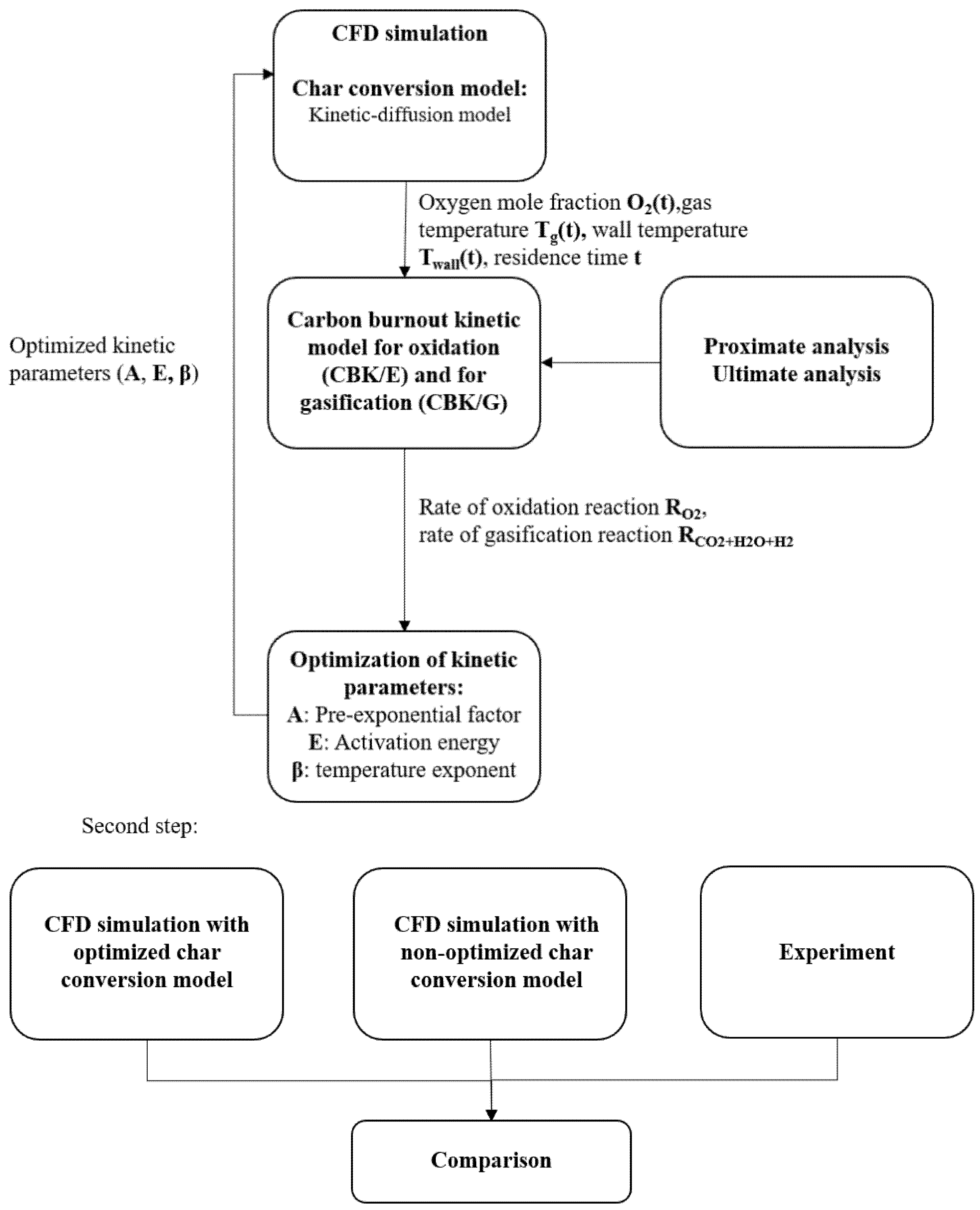
3. Optimization Procedure

The main idea of the optimization procedure is presented in Figure 1. At first, a CFD simulation is carried out with literature-taken kinetic parameters for the global kinetic-diffusion model. In the next step, CFD results provide specific input data for CBK, such as O₂% volume distribution, gas temperature, wall temperature, and particle residence time. Additionally, operating pressure, fuel properties from proximate and ultimate analyses and particle size are provided. It must be mentioned that CBK can handle only monodisperse particles. Therefore only the mean particle size was investigated. The main results of interest are the reaction rate of char-O₂ (obtained from CBK/E), one reaction rate as the sum of char-CO₂, char-H₂O, and char-H₂ reactions (obtained from CBK/G), and char conversion factor due to the oxidation reaction and overall gasification reaction. Afterwards, an optimization of kinetic parameters (activation energy, pre-exponential factor, temperature exponent) is performed through the minimization of the objective function (Equation (5)). Newly obtained pre-exponential factor, activation energy, and temperature exponents are further applied into CFD. The second step of the procedure considered the comparison of the results with optimized kinetic parameters and non-optimized (literature-taken) parameters based on the experimental data.

$$\mathrm{OF}\left({\mathrm{x}}_{\mathrm{k}}\right)=\frac{{{\displaystyle \sum }}_{\mathrm{j}=1}^{{\mathrm{N}}_{\mathrm{t},\mathrm{j}}}{\left({\mathrm{R}}_{\mathrm{i},\mathrm{j}}^{\mathrm{net}}-{\mathrm{R}}_{\mathrm{i},\mathrm{j}}^{\mathrm{emp}}\left({\mathrm{x}}_{\mathrm{k}}\right)\right)}^2}{{\mathrm{N}}_{\mathrm{t},\mathrm{i}}}$$

(5)

where: ${\mathrm{R}}^{\mathrm{net}}$ is the reaction rate from the complex models (CBK/E and CBK/G), ${\mathrm{x}}_{\mathrm{k}}$ are the model parameters (the pre-exponential factor, activation energy, temperature exponent), ${\mathrm{N}}_{\mathrm{t},\mathrm{j}}$ is the number of discrete time steps. The solution is obtained based on the Levenberg-Marquardt fitting routine. ${\mathrm{R}}^{\mathrm{emp}}$ is the reaction rate from the empirical model (Equation (2)).

It is important to mention that the objective function is calculated twice. One case considers oxidation, whereas the second case, gasification. The reaction rate from CBK/E is given in g/cm²-s. The reaction rate from CBK/G is given in 1/s. Therefore, it is necessary to convert the rate into g/cm²-s. The following relationship has been applied [21,54]:

$${\mathrm{R}}^{\mathrm{net}}\left[\frac{\mathrm{g}}{{\mathrm{cm}}^2\mathrm{s}}\right]=\frac{{\mathsf{\rho }}_{\mathrm{c}}{\mathrm{d}}_{\mathrm{p}}}{6\left(1-\mathrm{X}\right)}{\mathrm{R}}^{\mathrm{net}}\left[\frac{1}{\mathrm{s}}\right]$$

(6)

where ρ_c is the particle density, X is the conversion degree factor. Particle density and char conversion are also obtained from the CBK/G model. The reason why this is a two-step process lies in the fact that the char-O₂ reaction completely dominates the gasification process as long as the O₂ concentration is greater than approximately 500 ppm [20,21]. Therefore char combustion and char gasification are considered to occur consecutively.

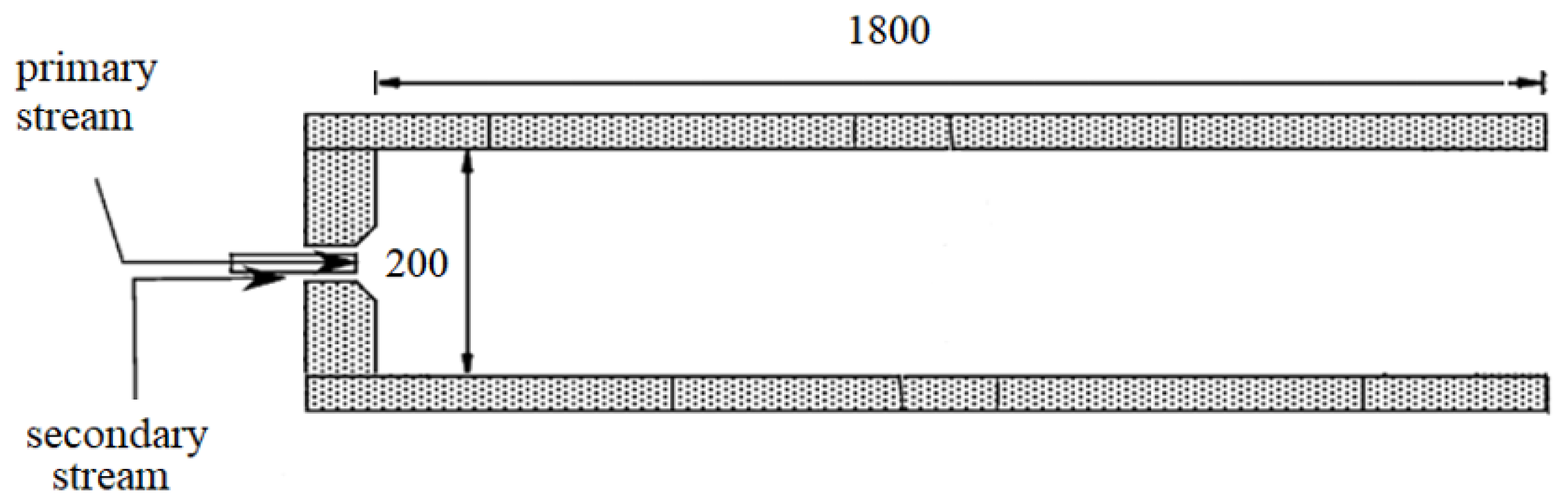
4. Reactor. Computational Domain

The Brigham Young University (BYU) reactor is a one-stage entrained-flow reactor operated with oxygen under 1 atm (Figure 2). It is 1.8 m long and has a diameter of 0.2 m. Pulverized bituminous Utah coal was used in the investigations. The ultimate and proximate analyses are presented in

Table 2. Proximate and ultimate analyses of Utah coal [36].

Proximate Analysis, % as Received
Volatile matter	45.6
Fixed carbon	43.7
Ash	8.3
Moisture	2.4
Ultimate Analysis, % Dry-Ash-Free
C	77.6
H	6.56
N	1.42
S	0.55

.

Coal was supplied in the primary stream with a gas composed of O₂, Ar, and H₂O. The secondary stream contained only H₂O. The mass flow rates with molar fractions of the gas components are presented in

Table 3. Mass flow rates of coal and gas with molar composition for BYU reactor.

1st Stream, kg/h	26.24
O2	0.85
Ar	0.126
H2O	0.024
2nd Stream, kg/h	6.62
H2O	1
Utah Bituminous Coal, kg/h	23.88

. The particle size followed the Rosin-Rammler distribution where the mass fraction of particles of diameter greater than d is given by:

$${\mathrm{Y}}^{\mathrm{d}}={\mathrm{e}}^{-{\left(\frac{\mathrm{d}}{\mathrm{d}}\right)}^{\mathrm{n}}}$$

(7)

where $\overline{\mathrm{d}}$ is the mean diameter, n is the spread parameter.

The parameters applied in this study are presented in

Table 4. Parameters used for Rosin Rammler distribution.

Min. Diameter	Max. Diameter	Mean Diameter	Spread Parameter
dmin, µm	dmax, µm	$\overline{\mathrm{d}}$, µm	n
1	85	36	1.033

. The kinetic parameters of devolatilization and homogeneous reactions are presented in

Table 5. Kinetic parameters for devolatilization and gas-phase reactions (global reaction approach).

Reactions:	Kinetic Parameters: A—kg/s Pa, E—J/kmol, α—No Unit
Devolatilization:
Vol → 0.218C7H10.61O0.87 + 0.322CH6.33 + 0.309H2O + 0.127CO + 0.024CO2 x = 7, y = 10.61, z = 0.87 m = 1, n = 6.33	${\mathrm{A}}_1=\mathrm{42,690}$ ${\mathrm{E}}_1=3.71\times {10}^7$ ${\mathsf{\alpha }}_1=0.246$ ${\mathrm{A}}_2=9.785\times {10}^6$ ${\mathrm{E}}_2=8.993\times {10}^7$ ${\mathsf{\alpha }}_2=0.931$
Gas-Phase Reactions:
${\mathrm{C}}_{\mathrm{x}}{\mathrm{H}}_{\mathrm{y}}{\mathrm{O}}_{\mathrm{z}}+\frac{\mathrm{x}-\mathrm{z}}{2}{\mathrm{O}}_2\to \mathrm{xCO}+\frac{\mathrm{y}}{2}{\mathrm{H}}_2$	$\mathrm{A}=4.4\times {10}^{11}$ $\mathrm{E}=1.25\times {10}^8$ [42]
${\mathrm{C}}_{\mathrm{x}}{\mathrm{H}}_{\mathrm{y}}{\mathrm{O}}_{\mathrm{z}}+\left(\mathrm{x}-\mathrm{z}\right){\mathrm{H}}_2\mathrm{O}\to \mathrm{xCO}+\left(\frac{\mathrm{y}}{2}+\mathrm{x}-\mathrm{z}\right){\mathrm{H}}_2$	$\mathrm{A}=3\times {10}^8$ $\mathrm{E}=1.25\times {10}^8$ [42]
${\mathrm{C}}_{\mathrm{m}}{\mathrm{H}}_{\mathrm{n}}+\frac{\mathrm{m}}{2}{\mathrm{O}}_2\to \mathrm{mCO}+\frac{\mathrm{n}}{2}{\mathrm{H}}_2$	$\mathrm{A}=4.4\times {10}^{11}$ $\mathrm{E}=1.25\times {10}^8$ [42]
${\mathrm{C}}_{\mathrm{m}}{\mathrm{H}}_{\mathrm{n}}+{\mathrm{H}}_2\mathrm{O}\to \mathrm{mCO}+\left(\frac{\mathrm{n}}{2}+1\right){\mathrm{H}}_2$	$\mathrm{A}=3\times {10}^8$ $\mathrm{E}=1.25\times {10}^8$ [42]
$\mathrm{CO}+{\mathrm{H}}_2\mathrm{O}\to {\mathrm{CO}}_2+{\mathrm{H}}_2$	$\mathrm{A}=2.75$ [46] $\mathrm{E}=8.38\times {10}^7$ [55]
$\mathrm{CO}+0.5{\mathrm{O}}_2\to {\mathrm{CO}}_2$	$\mathrm{A}=2.24\times {10}^{12}$ $\mathrm{E}=1.67\times {10}^8$ [56]
${\mathrm{H}}_2+0.5{\mathrm{O}}_2\to {\mathrm{H}}_2\mathrm{O}$	$\mathrm{A}=6.8\times {10}^{15}$ $\mathrm{E}=1.67\times {10}^8$ [42] β = −1

. The reactor geometry was discretized applying a 2-D axisymmetric grid consisting of approximately 100,000 rectangular cells. A grid independence study was carried out. For further information regarding the model please refer to the supplementary data. The numerical simulation was validated against the experimental data of Smith et al. [36] who measured gas-phase concentrations of CO, H₂, and CO₂ at different axial and radial locations using isokinetic probes. H₂O concentration was calculated on the basis of the hydrogen elemental balance. This calculation, however, leads to an ±14% uncertainty owing to the reported uncertainty in the char ash analysis [36], especially in the flame region. Therefore, the model quality estimation with regard to the experimental data should only be performed for CO, H₂, and CO₂.

The reaction kinetics of C_xH_yO_z and C_mH_n with O₂ and H₂O were assumed to be identical to those of light hydrocarbon molecules, such as CH₄ [42]. The choice is justified because these reaction rates do not vary greatly [55,56].

Table 6. Kinetic parameters for surface reactions.

Reactions	Kinetic Parameters A—kg/s Pa E—J/kmol β—No Unit	Literature Parameters No. 1 [30]	Optimized Parameters Based on CBK/E and CBK/G Models	Literature Parameters No. 2 [42]	Literature Parameters No. 3 [15]	Literature Parameters No. 4 [15]
C + 0.5O2 → CO	A	0.052	$1.298\times {10}^{-3}$	2.3	0.005	0.005
	E	$6.1\times {10}^7$	$1.324\times {10}^8$	$9.23\times {10}^7$	$7.4\times {10}^7$	$7.4\times {10}^7$
	β	0	1.233	1	0	0
C + CO2 → 2CO	A	$0.0732$	0.066	4.4	0.3493	0.0635
	E	$1.125\times {10}^8$	$1.385\times {10}^8$	$1.62\times {10}^8$	$2.36\times {10}^8$	$1.62\times {10}^8$
	β	0	−0.263	1	0	0
C + H2O → CO + H2	A	0.0782	$1.877\times {10}^{-3}$	1.33	61.484	0.0019
	E	$1.5\times {10}^8$	$1.588\times {10}^8$	$1.47\times {10}^8$	$3.16\times {10}^8$	$1.47\times {10}^8$
	β	0	−0.124	1	0	0

presents four sets of widely applied literature-taken kinetic parameters and one set of parameters, which was obtained through the optimization procedure.

5. Results

The results are divided into two parts. The first part considers the results from the optimization procedure. The second part regards the CFD results.

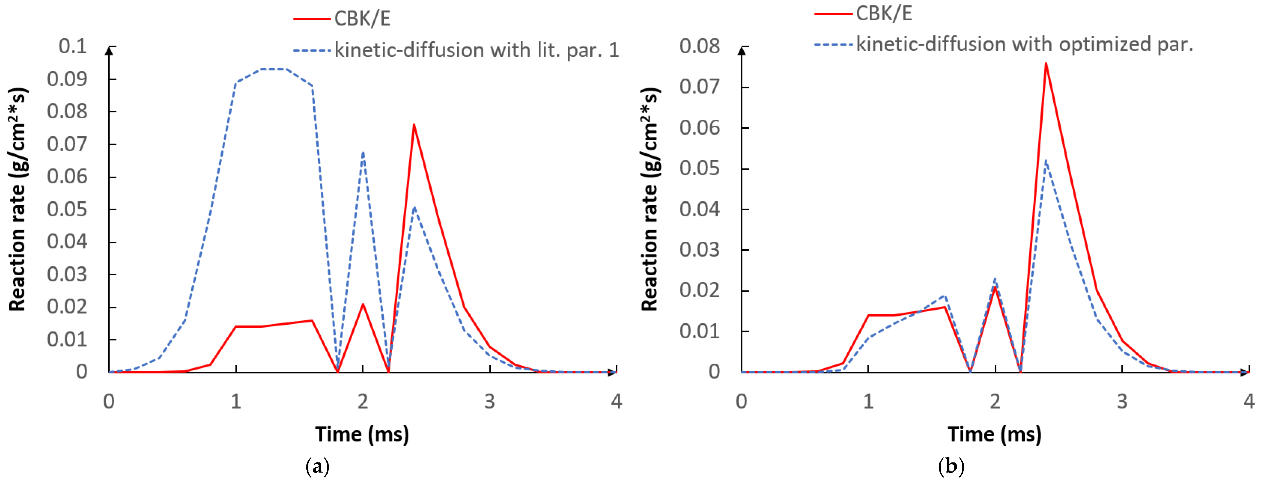
5.1. Optimization Procedure Results

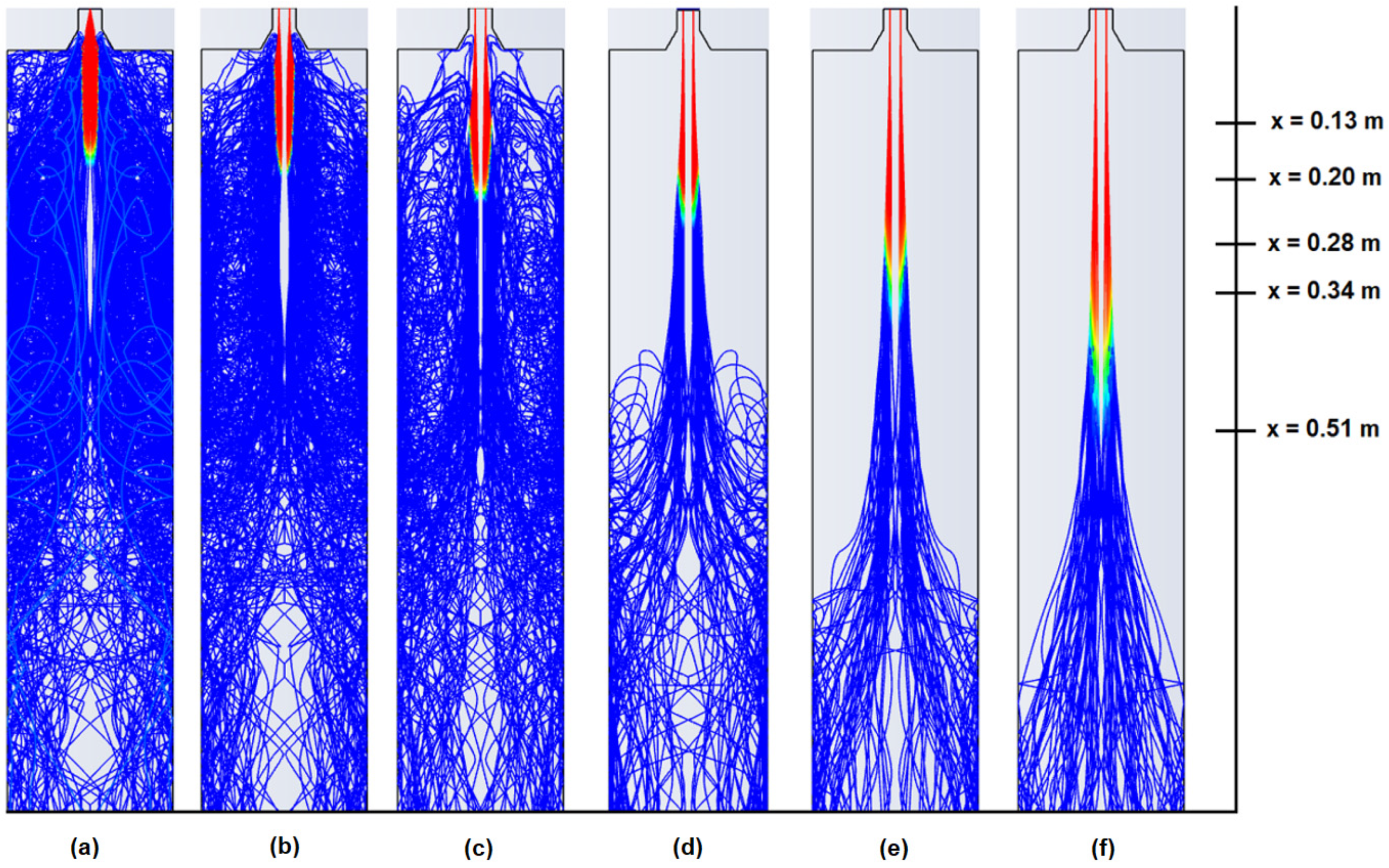
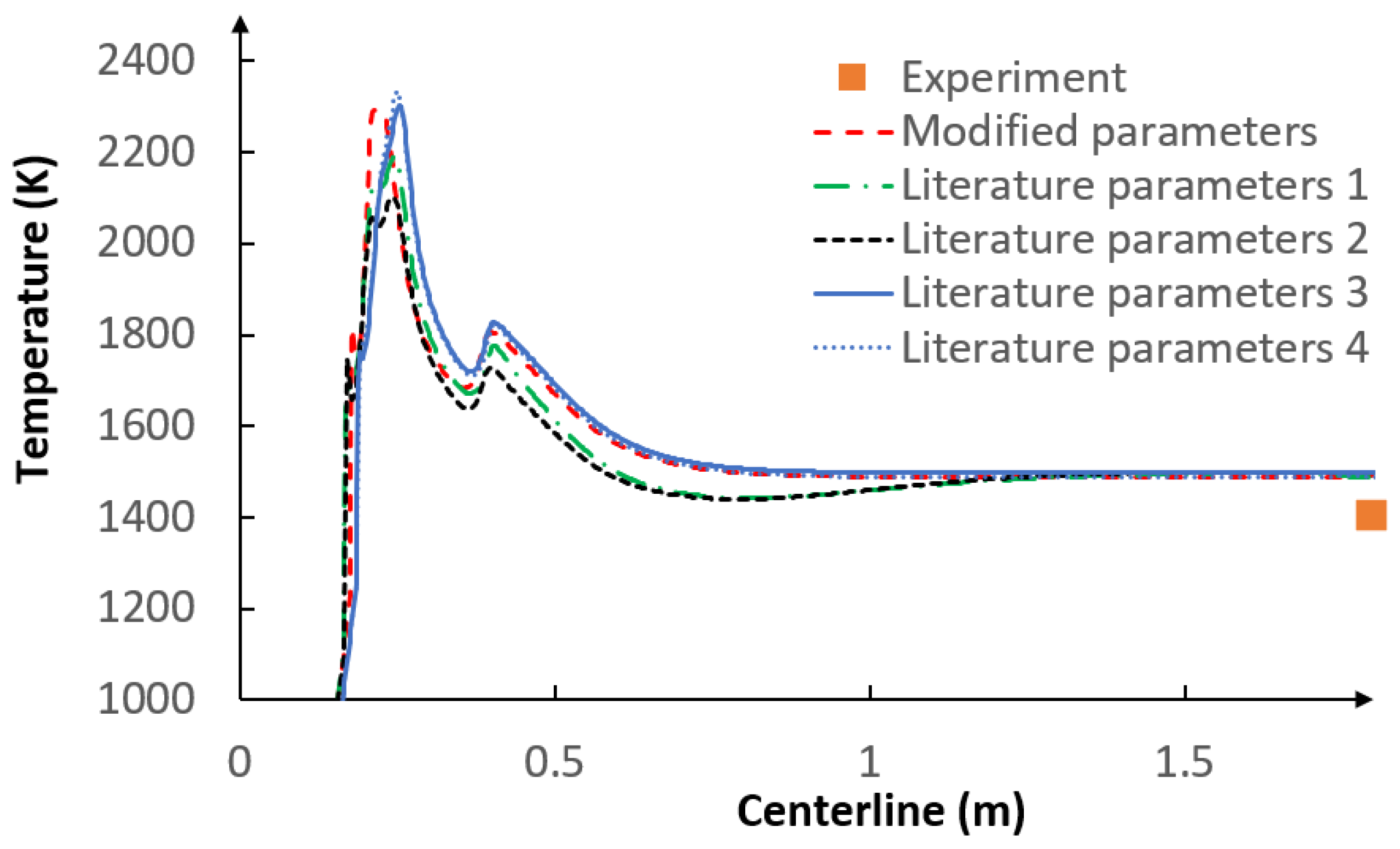
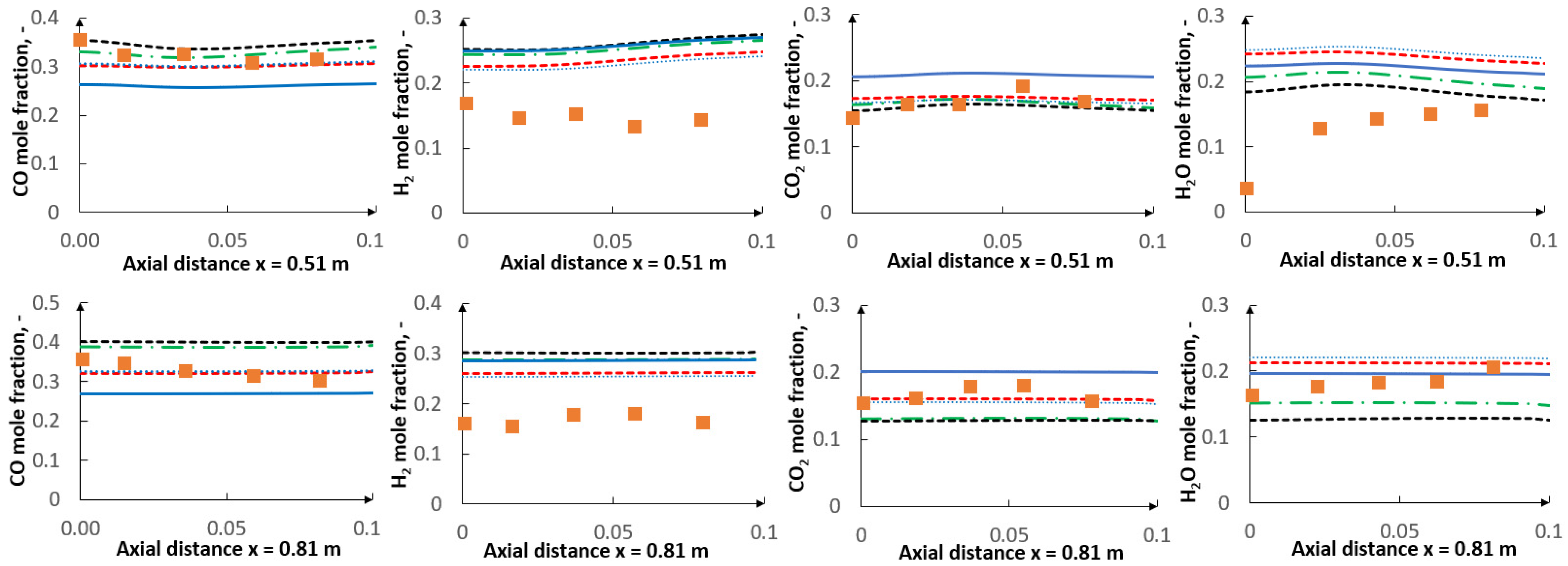
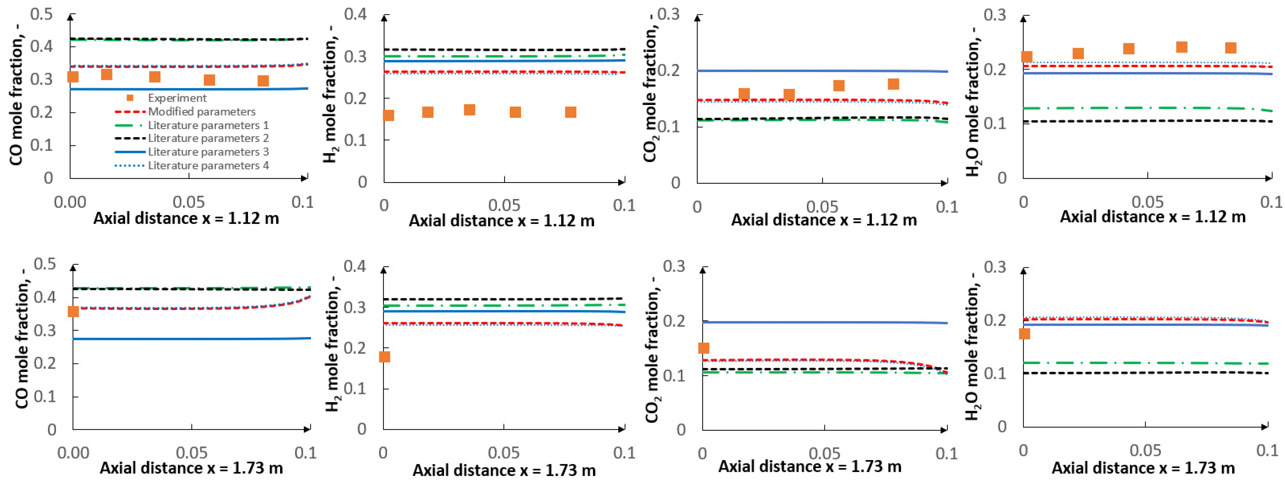
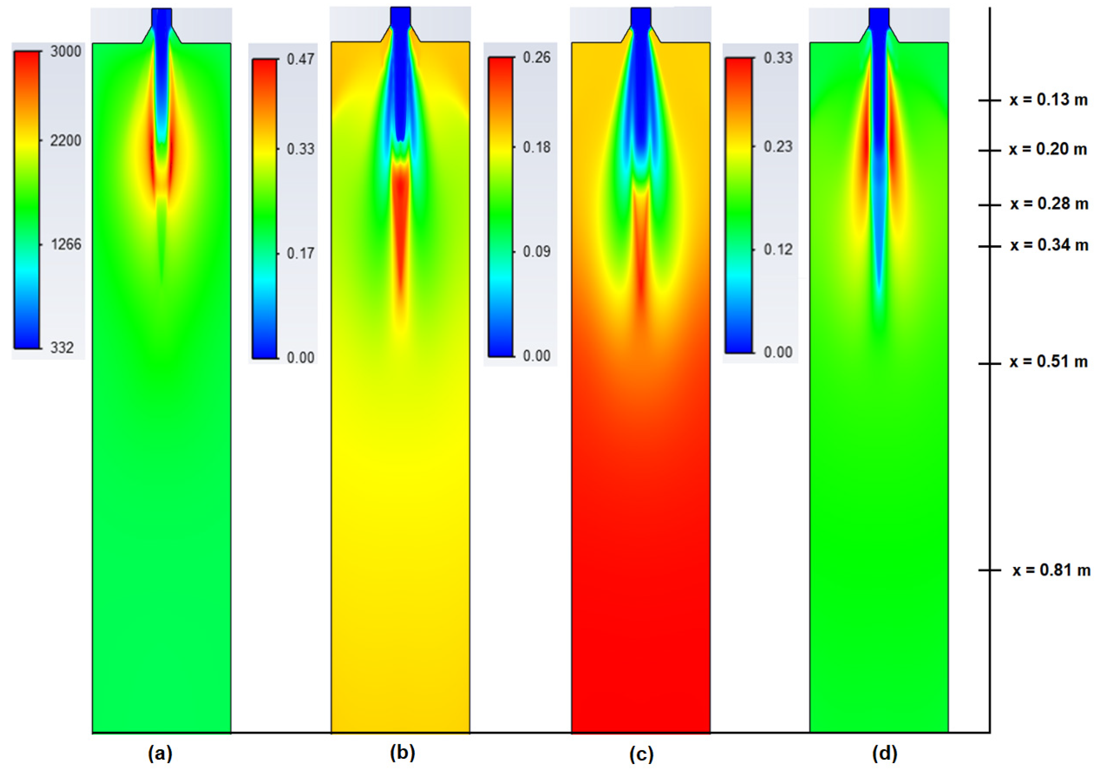
The results consider the optimization of kinetic parameters for the kinetic-diffusion model based on the reaction rates obtained from the CBK/E and CBK/G models. Figure 3a presents the reaction rates from CBK/E and the kinetic-diffusion model with literature-taken kinetic parameters 1 [30]. One can notice that the O₂ consumption rate is strongly overpredicted by the kinetic-diffusion model with literature-taken kinetic parameters with respect to the detailed CBK/E approach, especially up to 2.2 ms. Figure 3b depicts optimized reaction rates of the kinetic-diffusion model based on CBK/E results. One can observe a relatively reasonable agreement. The final coefficient of determination is equal to 96.1%. In comparison with, e.g., intrinsic-based char conversion models, the kinetic-diffusion approach is a relatively simple model, and therefore extremely high coefficients of determination for this approach were not possible.

As regards the optimization of the gasification step, the first phase in the optimization process required proper estimation of the frequency factor for surface oxide desorption in the CBK/G model [21]. The CBK/G version implemented into NEA’s PC Coal lab accounts for an empirical correlation, linking the kinetic parameters in the model with the daf carbon content of the parent coal [57]:

$${\mathrm{A}}_{70}={10}^{0.1{\mathrm{C}}_{\mathrm{daf}}-0.64}$$

(8)

where A₇₀ is the frequency factor, C_daf is coal carbon content in dry-ash-free (daf) wt.%.

However, while analyzing the performance of CBK/G for a dataset of 228 coals with char conversion in the range from 0% to 100%, a significant scatter with respect to the experiments was observed. It concerned especially low and high conversion levels. It was concluded that the above empirical relation only depicted the overall tendency in the gasification reactivity with the coal rank. Therefore, it was suggested to adjust all the kinetic rates proportionally to the rate of the CO desorption (C (O) $\to$ CO) to obtain the most accurate match with experiments. As a result, instead of applying Equation (8), the frequency factor was scaled on the basis of the char conversion experiment of the Illinois coal [58], which is close to that analyzed in the present study of Utah coal, was based on the Van Krevelen diagram (Figure 4).

Figure 5 presents the results of the CBK/G model with the frequency factor obtained from Equation (8), and with the adjusted frequency factor on the basis of the experimental data [58]. Judging by the results, the modified frequency factor will be further incorporated in the calculations.

Figure 6a presents the gasification reaction rate of CBK/G and the reaction rate of the kinetic-diffusion model with literature-taken parameters no. 1 [30]. Owing to the fact that the reaction rate from CBK/G is actually the sum of char-CO₂, char-H₂O, and char-H₂ rates, the overall gasification rate for the empirical kinetic-diffusion model was formulated as the sum of char-CO₂ and char-H₂O rates. Based on the literature, the char-H₂ reaction rate is generally very low compared to the other gasification reactions. Therefore its impact was neglected in the empirical model. The final gasification reaction rate for the empirical kinetic-diffusion model is therefore defined as follows:

$${\mathrm{R}}_{{\mathrm{CO}}_2+{\mathrm{H}}_2\mathrm{O}+{\mathrm{H}}_2}={\mathrm{R}}_{{\mathrm{CO}}_2}+{\mathrm{R}}_{{\mathrm{H}}_2\mathrm{O}}$$

(9)

The choice is relevant because at atmospheric pressures separated active sites for CO₂ and H₂O can be assumed and consequently, the total reaction rate can be the sum of the individual rates [59,60,61]. Based on Figure 6, one can notice a strong overprediction by the kinetic-diffusion model with literature-taken kinetic parameters no. 1. In such a case, the char conversion factor would be strongly overpredicted. The figure clearly indicates that applying literature kinetic parameters can lead to substantial errors. Figure 6b depicts the optimized global model based on the results of CBK/G. In this case, a coefficient of determination is equal to 97.2%. The optimized kinetic parameters can be found in Table 6.

Figure 7 depicts the reaction rate of char oxidation for the kinetic-diffusion model with literature parameters from Table 6 and CBK/E, whereas Figure 8 depicts the reaction rate of char gasification for the kinetic-diffusion model with literature parameters from Table 6, and for CBK/G. One can observe a very strong impact of the applied parameters on the reaction rate. In Figure 8 the results have been presented in two sub-figures because the reaction rates with literature parameters no. 3 and no. 4 are an order of magnitude smaller than for parameters no. 1 and no. 2. It is clear that prior to any simulation, char conversion parameters have to be carefully adjusted in order to accurately predict the behavior of the rate of surface reactions.

5.2. CFD Results

This sub-section presents the CFD results for the BYU reactor focusing on the char conversion aspect. Four sets of literature-taken kinetic parameters and one set of optimized parameters based on the CBK/E and CBK/G models are analyzed. Figure 9 presents the molar fraction concentrations of CO, H₂, CO₂, and H₂O along the centerline of the BYU reactor.

An extreme impact of the applied char conversion kinetic parameters on the overall gas composition can be observed. One can notice that the slope of the curves varies in the reforming zone which corresponds to the strength of the gasification reactions. Judging by Figure 7 and Figure 8, the second set of kinetic parameters provides the highest reaction rate. As a result, in Figure 9 for the second set of kinetic parameters the CO and H₂ mole fraction curves have the highest slopes in the reforming zone and consequently, the highest amount of CO and H₂ produced, while they have the lowest amount of CO₂ and H₂O. As for the third set of kinetic parameters, the gasification rate is the slowest (Figure 7 and Figure 8), hence the lowest slope of the CO mole fraction curve in the reforming zone can be observed and the smallest amount of the final CO produced. One can notice that the optimized kinetic parameters and the fourth set of literature-taken parameters are the most accurate ones with respect to the experimental results. The phenomenon that a given set of data can be fitted equally well by more than one pair of kinetic parameters is referred to as the compensation effect. This was already mentioned by [62,63,64,65]. The impact of gasification reactions is less pronounced in the lean zone and at the beginning of the flame zone where devolatilization and char oxidation prevail. However, the contribution of these reactions in these zones is also non-negligible. Figure 10 depicts the devolatilization process of particles with 6 representative diameters. For clarity, each sub-figure consists of 50 particles. A considerable influence of the particle diameter on the onset of devolatilization and the overall time of devolatilization can be observed. The sooner the volatiles are released, the sooner the surface reactions begin to occur. One can notice that the axial distance for which the volatiles are released varies from x = 0.2 m to x = 0.5 m. Therefore, different kinetics of the surface reactions will result in different strength of the surface reactions in this region. As a result, different amounts of CO, H₂, CO₂, and H₂O are to be expected. Judging by Figure 10a–c, it is also evident that for smaller particles recirculation is much more intense.

Judging by Figure 11, the applied kinetic parameters have also a non-negligible effect on the temperature distribution inside the reactor. Due to more intensive gasification reactions for the literature parameters no. 2 and no. 3, because of their endothermic character, the temperature is substantially lower, especially in the reforming zone, where gasification reactions dominate.

Table 7. CFD results: char conversion degree for surface reaction model with different kinetic parameters with regard to experiments.

Char Conversion Degree %
	Simulation Results Mean Particle Diameter 36 µm	Simulation Results All Particle Fractions 1–85 µm	Experiment All Particle Fractions 1–85 µm
Literature parameters 1	100%	100%	82%
Optimized parameters	83%	77%
Literature parameters 2	100%	99%
Literature parameters 3	27%	59%
Literature parameters 4	80%	74%

presents the char conversion factor results for the kinetic-diffusion model with kinetic parameters from Table 6. As was already mentioned, CBK/E and CBK/G models can handle only monodisperse particles. Therefore the optimized kinetic parameters inherently correspond to the mean particle diameter. On this basis, Table 7 regards both the mean particle diameter comparison and all particle fractions with regard to the experiment. Judging by the results, the optimized kinetic parameters for the mean particle diameter are in excellent agreement with the experiment. Char conversion factors for all particle fractions for the optimized parameters and literature parameters no. 4 are in close agreement with the experiment. Future enhancement of CBK/E and CBK/G models to account for polydisperse particles would improve the accuracy of simulations, providing more exact reaction rates. As a result, optimized kinetic parameters would directly correspond to all particle fractions.

The accuracy of the optimization procedure for the axial in-reactor gas composition (Figure 9) has been additionally assessed with error analysis. A maximum and average value of absolute errors for non–optimized and optimized models are presented. The absolute error is defined as:

$$\Delta \mathrm{e}=\left|{\mathrm{x}}_{\exp }-{\mathrm{x}}_{\mathrm{num}}\right|$$

(10)

where ${\mathrm{x}}_{\exp }$ and ${\mathrm{x}}_{\mathrm{num}}$ are the experimental and numerical values of the specific variables (e.g., CO/H₂/CO₂/H₂O mole fraction), respectively.

Table 8. Error analysis of CO, H₂, CO₂ and H₂O concentration along the centerline (Figure 9).

Kinetic Parameters	CO		H2		CO2		H2O
	Max Δe (%)	Av. Δe (%)	Max Δe (%)	Av. Δe (%)	Max Δe (%)	Av. Δe (%)	Max Δe (%)	Av. Δe (%)
Lit. parameters 1	17.91	6.74	12.80	7.89	10.22	5.87	16.82	11.84
Mod. parameters	18.48	4.82	7.95	5.47	10.15	4.72	20.22	9.58
Lit. parameters 2	20.20	7.94	14.40	8.98	10.15	5.98	19.73	13.04
Lit. parameters 3	11.11	5.71	11.36	7.51	10.14	5.38	19.24	10.35
Lit. parameters 4	12.50	4.90	8.33	5.40	10.16	4.77	20.68	8.99

presents the quantitative assessment of the procedure. Judging by the results, the application of the modified parameters and literature parameters no. 4 results in one of the lowest errors with respect to the experimental data.

Figure 12, Figure 13 and Figure 14 present molar fraction gas concentrations along radial traverses for axial distances x = 0.13 m, x = 0.20 m, x = 0.28 m, x = 0.34 m, x = 0.51 m, x = 0.81 m, x = 1.12 m and x = 1.73 m. These traverses are visualized in Figure 15. In most cases, the model results with the optimized kinetic parameters are in closest agreement with experimental data. As mentioned, H₂O mole fraction results are calculated from hydrogen balance and should not be considered as credible reference data. The impact of the applied parameters on the radial distribution is less substantial than for the axial distribution. This observation is sensible because the gasification reactions that dominate the reforming zone proceed axially along with the mainstream. Another observation regards the changes in radial concentration. One may notice that from the axial distance x = 0.51 m, the molar distribution of species stabilizes in the radial direction. There are insignificant changes in the yield. This means that after the devolatilization process, gasification reactions, which begin to dominate in the reforming zone, are radially uniform. On the other hand, substantial changes in the radial direction (Figure 12 and Figure 13) for the axial distances x < 0.51 m can be observed. These changes are most abrupt up to the radial distance 0.04 m where the boundary of the flame is located (Figure 16).

Figure 17 shows the contour plots of temperature, CO, H₂, and CO₂ mole fractions, while Figure 18 presents the contour plots of H₂O, O₂ mole fractions, and the devolatilization reaction rate. Five regions can be noticed in the reactor: the lean zone, the recirculation zone, the flame zone, the post-flame zone, and the reforming zone. In the lean zone, equivalence ratios are lower than stoichiometric conditions, which corresponds to high O₂ content (Figure 18b). This zone is mainly composed of O₂ and H₂O, which are introduced in the primary and secondary streams. The flame zone begins downstream of the lean zone, reaching very high temperatures–3000 K—owing to the high O₂ content in the primary stream. CO and H₂ content are relatively low. In the post-flame zone, which follows the flame zone, the temperatures are lower than in the flame. This region is also characterized by a very rich mixture. CO and H₂ are mainly formed in this region because of the combined effect of the water–gas shift reaction and the gasification reactions. The next zone is dominated by reforming reactions. In this region, there are lower temperatures, extremely small gradients, and low conversion rates. CO and H₂ continue to increase slowly approaching the equilibrium conditions. The last region is characterized by a strong recirculation of the gas and coal particles, the recirculation zone. This is located between the lean, flame, post-flame zones and the reactor wall.

6. Conclusions

An optimization procedure for the empirical char conversion kinetic-diffusion model, based on the detailed CBK/E and CBK/G models, was presented. The numerical model was validated against the experimental data from the BYU gasifier. The BYU reactor reference measurements are suitable for this purpose since in-reactor measurement data are available which is vital when one considers the credible and effective assessment of the predictive capabilities of the CFD model. The following main conclusions can be drawn:

• The optimization procedure investigated in the current allows enhancing the modeling strategy by obtaining adjusted kinetic parameters of the kinetic-diffusion model only for the specific operating conditions.
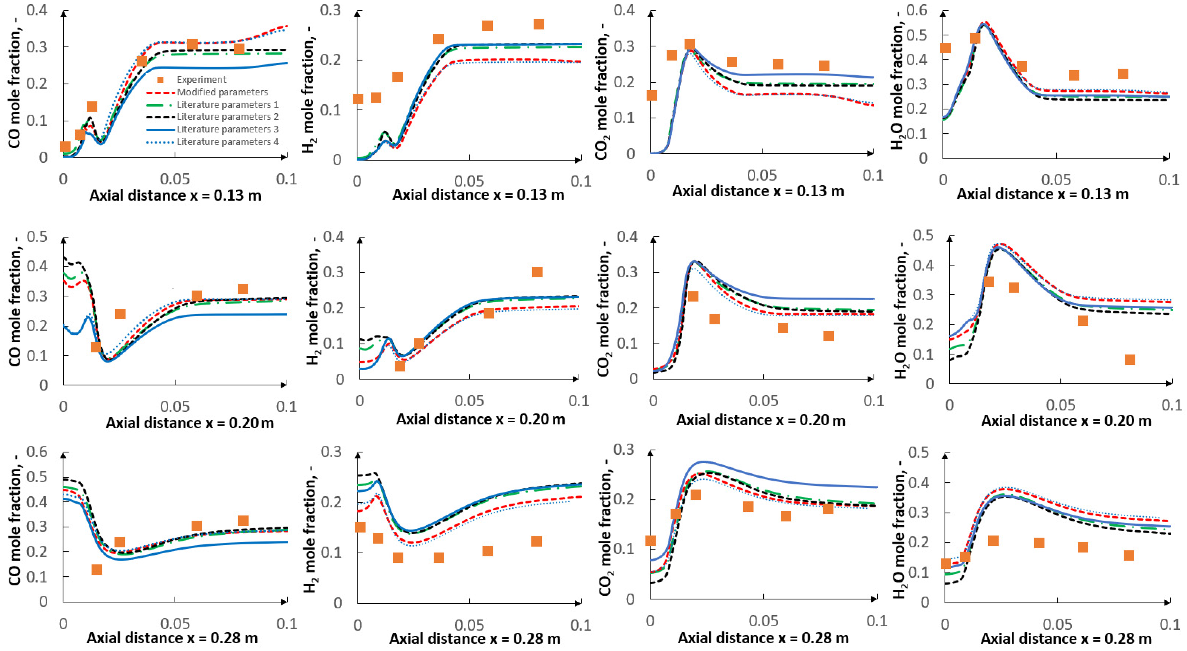
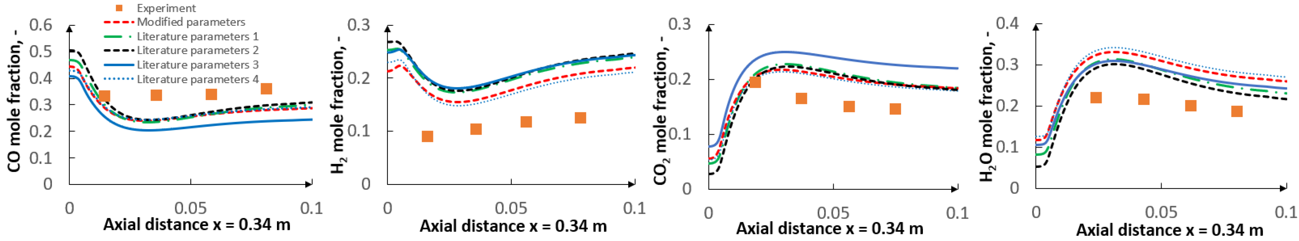
• The use of the optimization procedure resulted in a better agreement between the model results and the experimental data in terms of the gas composition and char conversion factor. In order to further improve the accuracy of the procedure, future research should consider the application of the intrinsic-based char conversion models with Langmuir-Hinshelwood (LH) kinetics.
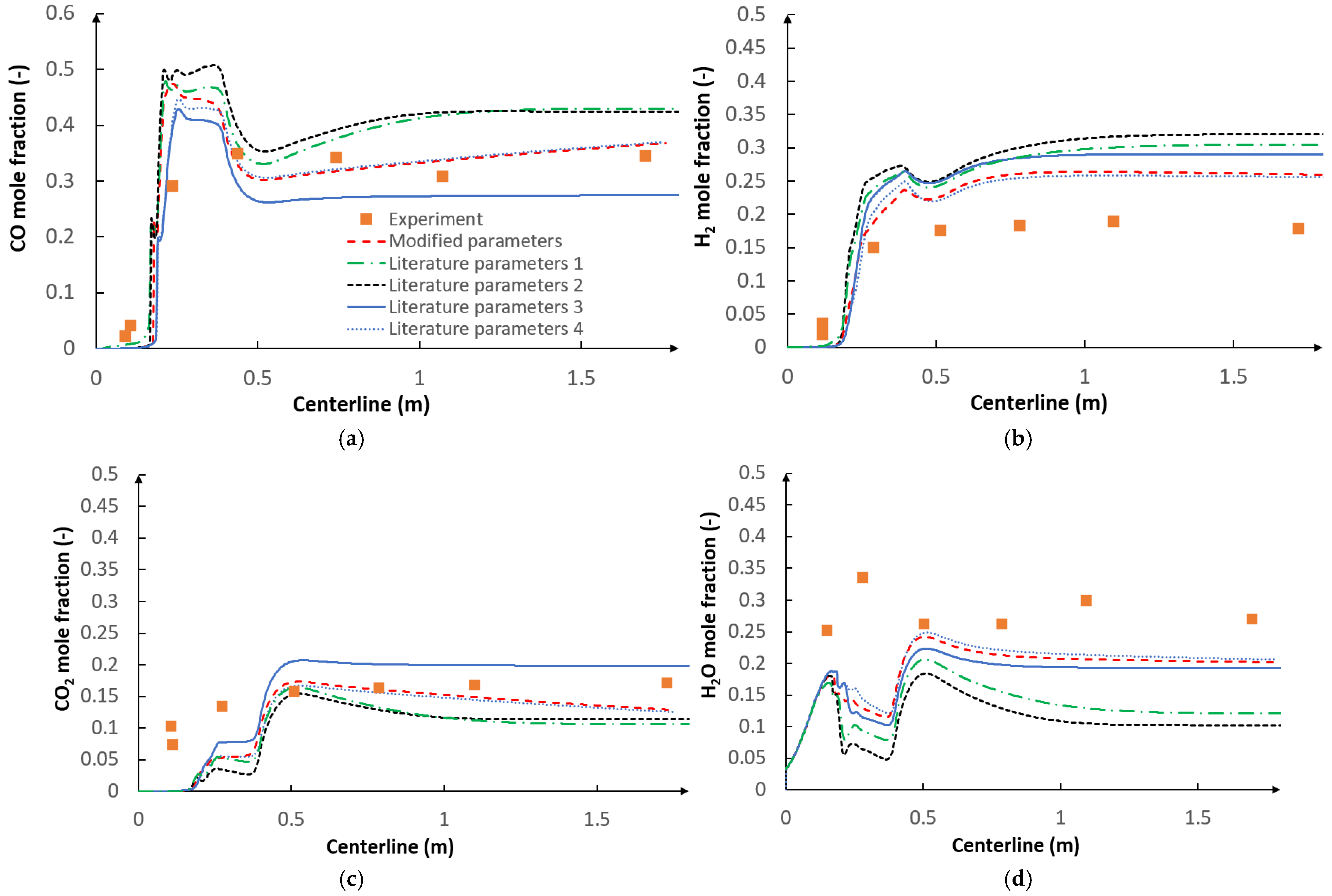
• The applied kinetic parameters of char-oxidation and char-gasification reactions proved to have a significant impact in the gasification process simulations. The major effect could be observed on the final gas composition and the char conversion factor, but also on the gas composition in the flame zone.
• Due to the versatile character of the method, the presented optimization procedure can be applied in other areas of interest, provided that both complex and simple models are available.

References

1. EIA. Today in Energy—U.S. Energy Information Administration (EIA). Available online: https://www.eia.gov/todayinenergy/detail.php?id=26912 (accessed on 8 October 2020).
2. Worldometer. World Coal Statistics—Worldometer. Available online: https://www.worldometers.info/coal/ (accessed on 8 October 2020).
3. IEA. Emissions—Global Energy & CO2 Status Report 2019—Analysis. Available online: https://www.iea.org/reports/global-energy-co2-status-report-2019/emissions (accessed on 8 October 2020).
4. Pawlak-Kruczek, H.; Wnukowski, M.; Niedzwiecki, L.; Czerep, M.; Kowal, M.; Krochmalny, K.; Zgóra, J.; Ostrycharczyk, M.; Baranowski, M.; Tic, W.J.; et al. Torrefaction as a valorization method used prior to the gasification of sewage sludge. Energies 2019, 12, 175. [Google Scholar] [CrossRef] [Green Version]
5. Luo, H.; Niedzwiecki, L.; Arora, A.; Mościcki, K.; Pawlak-Kruczek, H.; Krochmalny, K.; Baranowski, M.; Tiwari, M.; Sharma, A.; Sharma, T.; et al. Influence of torrefaction and pelletizing of sawdust on the design parameters of a fixed bed gasifier. Energies 2020, 13, 3018. [Google Scholar] [CrossRef]
6. NETL. IGCC Efficiency/Performance. Available online: https://www.netl.doe.gov/research/Coal/energy-systems/gasification/gasifipedia/igcc-efficiency (accessed on 10 February 2021).
7. Li, J.; Paul, M.C.; Younger, P.L.; Watson, I.; Hossain, M.; Welch, S. Combustion modelling of pulverized biomass particles at high temperatures. Phys. Procedia 2015, 66, 273–276. [Google Scholar] [CrossRef] [Green Version]
8. Klimanek, A.; Adamczyk, W.P.; Katelbach-Woźniak, A.; Węcel, G.; Szlęk, A. Towards a hybrid Eulerian–Lagrangian CFD modeling of coal gasification in a circulating fluidized bed reactor. Fuel 2015, 152, 131–137. [Google Scholar] [CrossRef]
9. Drikakis, D.; Frank, M.; Tabor, G. Multiscale computational fluid dynamics. Energies 2019, 12, 3272. [Google Scholar] [CrossRef] [Green Version]
10. Della Torre, A.; Montenegro, G.; Onorati, A.; Khadilkar, S.; Icarelli, R. Multi-scale CFD modeling of plate heat exchangers including offset-strip fins and dimple-type turbulators for automotive applications. Energies 2019, 12, 2965. [Google Scholar] [CrossRef] [Green Version]
11. Sutardi, T.; Wang, L.; Karimi, N.; Paul, M.C. Utilization of H2O and CO2 in coal particle gasification with an impact of temperature and particle size. Energy Fuels 2020, 34, 12841–12852. [Google Scholar] [CrossRef]
12. Pour, M.S.; Weihong, Y. Performance of pulverized coal combustion under high temperature air diluted by steam. ISRN Mech. Eng. 2014, 2014, 217574. [Google Scholar] [CrossRef] [Green Version]
13. Xu, J.; Qiao, L. Mathematical modeling of coal gasification processes in a well-stirred reactor: Effects of devolatilization and moisture content. Energy Fuels 2012, 26, 5759–5768. [Google Scholar] [CrossRef]
14. Mularski, J.; Modliński, N. Entrained flow coal gasification process simulation with the emphasis on empirical devolatilization models optimization procedure. Appl. Therm. Eng. 2020, 175, 115401. [Google Scholar] [CrossRef]
15. Vascellari, M.; Arora, R.; Pollack, M.; Hasse, C. Simulation of entrained flow gasification with advanced coal conversion submodels. Part 1: Pyrolysis. Fuel 2013, 113, 654–669. [Google Scholar] [CrossRef]
16. Mularski, J.; Modliński, N. Impact of Chemistry–Turbulence Interaction Modeling Approach on the CFD Simulations of Entrained Flow Coal Gasification. Energies 2020, 13, 6467. [Google Scholar] [CrossRef]
17. Mularski, J.; Pawlak-Kruczek, H.; Modlinski, N. A review of recent studies of the CFD modelling of coal gasification in entrained flow gasifiers, covering devolatilization, gas-phase reactions, surface reactions, models and kinetics. Fuel 2020, 271, 117620. [Google Scholar] [CrossRef]
18. Baum, M.M.; Street, P.J. Predicting the combustion behaviour of coal particles. Combust. Sci. Technol. 1971, 3, 231–243. [Google Scholar] [CrossRef]
19. Smith, I. The combustion rates of coal chars: A review. Symp. Combust. 1982, 19, 1045–1065. [Google Scholar] [CrossRef]
20. Niksa, S.; Liu, G.-S.; Hurt, R.H. Coal conversion submodels for design applications at elevated pressures. Part I. Devolatilization and char oxidation. Prog. Energy Combust. Sci. 2003, 29, 425–477. [Google Scholar] [CrossRef]
21. Liu, G.-S.; Niksa, S. Coal conversion submodels for design applications at elevated pressures. Part II. Char gasification. Prog. Energy Combust. Sci. 2004, 30, 679–717. [Google Scholar] [CrossRef]
22. Halama, S.; Spliethoff, H. Numerical simulation of entrained flow gasification: Reaction kinetics and char structure evolution. Fuel Process. Technol. 2015, 138, 314–324. [Google Scholar] [CrossRef]
23. Silaen, A.; Wang, T. Comparison of instantaneous, equilibrium, and finite-rate gasification models in an entrained-flow coal gasifier. In Proceedings of the 26th Annual International Pittsburgh Coal Conference 2009, Pittsburgh, PA, USA, 20–23 September 2009; pp. 1–11. [Google Scholar]
24. Lu, X.; Wang, T. Water–gas shift modeling in coal gasification in an entrained-flow gasifier—Part 2: Gasification application. Fuel 2013, 108, 620–628. [Google Scholar] [CrossRef]
25. Liu, H.; Kojima, T. Theoretical study of coal gasification in a 50 ton/day HYCOL entrained flow gasifier. I. Effects of coal properties and implications. Energy Fuels 2004, 18, 908–912. [Google Scholar] [CrossRef]
26. Liu, H.; Kojima, T. Theoretical study of coal gasification in a 50 ton/day HYCOL entrained flow gasifier. II. Effects of operating conditions and comparison with pilot-scale experiments. Energy Fuels 2004, 18, 913–917. [Google Scholar] [CrossRef]
27. Khan, J.R.; Wang, T. Implementation of a demoisturization and devolatilization model in multi-phase simulation of a hybrid entrained-flow and fluidized bed mild gasifier. Int. J. Clean Coal Energy 2013, 2, 35–53. [Google Scholar] [CrossRef]
28. Lu, X.; Wang, T. Investigation of radiation models in entrained-flow coal gasification simulation. Int. J. Heat Mass Transf. 2013, 67, 377–392. [Google Scholar] [CrossRef]
29. Lu, X.; Wang, T. Investigation of low rank coal gasification in a two-stage downdraft entrained-flow gasifier. Int. J. Clean Coal Energy 2014, 3, 1–12. [Google Scholar] [CrossRef] [Green Version]
30. Chen, C.; Horio, M.; Kojima, T. Numerical simulation of entrained flow coal gasifiers. Part I: Modeling of coal gasification in an entrained flow gasifier. Fuel 2000, 55, 3861–3874. [Google Scholar] [CrossRef]
31. Labbafan, A.; Ghassemi, H. Numerical modeling of an E-Gas entrained flow gasifier to characterize a high-ash coal gasification. Energy Convers. Manag. 2016, 112, 337–349. [Google Scholar] [CrossRef]
32. Chen, C.; Horio, M.; Kojima, T. Numerical simulation of entrained flow coal gasifiers. Part II: Effects of operating conditions on gasifier performance. Chem. Eng. Sci. 2000, 55, 3861–3874. [Google Scholar] [CrossRef]
33. Chen, C.; Horio, M.; Kojima, T. Use of numerical modeling in the design and scale-up of entrained flow coal gasifiers. Fuel 2001, 80, 1513–1523. [Google Scholar] [CrossRef]
34. Luan, Y.-T.; Chyou, Y.-P.; Wang, T. Numerical analysis of gasification performance via finite-rate model in a cross-type two-stage gasifier. Int. J. Heat Mass Transf. 2013, 57, 558–566. [Google Scholar] [CrossRef]
35. Ajilkumar, A.; Sundararajan, T.; Shet, U. Numerical modeling of a steam-assisted tubular coal gasifier. Int. J. Therm. Sci. 2009, 48, 308–321. [Google Scholar] [CrossRef]
36. Brown, B.W.; Smoot, L.D.; Smith, P.J.; Hedman, P.O. Measurement and prediction of entrained-flow gasification processes. AIChE J. 1988, 34, 435–446. [Google Scholar] [CrossRef]
37. Ansys Fluent—Fluid Simulation Software: User Guide 2020 (R2). Available online: https://ansyshelp.ansys.com/account/secured?returnurl=/Views/Secured/prod_page.html?pn=Fluent&prodver=20.2&lang=en (accessed on 9 March 2020).
38. Patankar, S.; Spalding, D. A calculation procedure for heat, mass and momentum transfer in three-dimensional parabolic flows. Int. J. Heat Mass Transf. 1972, 15, 1787–1806. [Google Scholar] [CrossRef]
39. Crowe, C.T.; Sharma, M.P.; Stock, D.E. The particle-source-in cell (PSI-CELL) model for gas-droplet flows. J. Fluids Eng. 1977, 99, 325–332. [Google Scholar] [CrossRef]
40. Shih, T.-H.; Liou, W.W.; Shabbir, A.; Yang, Z.; Zhu, J. A new k-ϵ eddy viscosity model for high reynolds number turbulent flows. Comput. Fluids 1995, 24, 227–238. [Google Scholar] [CrossRef]
41. Dukowicz, J.K. A particle-fluid numerical model for liquid sprays. J. Comput. Phys. 1980, 35, 229–253. [Google Scholar] [CrossRef]
42. Kumar, M.; Ghoniem, A.F. Multiphysics simulations of entrained flow gasification. Part II: Constructing and validating the overall model. Energy Fuels 2012, 26, 464–479. [Google Scholar] [CrossRef]
43. Kobayashi, H.; Howard, J.; Sarofim, A. Coal devolatilization at high temperatures. Symp. Combust. 1977, 16, 411–425. [Google Scholar] [CrossRef]
44. Magnussen, B.; Hjertager, B. On mathematical modeling of turbulent combustion with special emphasis on soot formation and combustion. Symp. Combust. 1977, 16, 719–729. [Google Scholar] [CrossRef]
45. Gosman, A.D.; Ioannides, E. Aspects of computer simulation of liquid-fuelled combustors. J. Energy 1983, 7, 482–490. [Google Scholar] [CrossRef]
46. Czajka, K.M.; Modliński, N.; Kisiela-Czajka, A.M.; Naidoo, R.; Peta, S.; Nyangwa, B. Volatile matter release from coal at different heating rates –experimental study and kinetic modelling. J. Anal. Appl. Pyrolysis 2019, 139, 282–290. [Google Scholar] [CrossRef]
47. Zhang, Z.; Lu, B.; Zhao, Z.; Zhang, L.; Chen, Y.; Li, S.; Luo, C.; Zheng, C. CFD modeling on char surface reaction behavior of pulverized coal MILD-oxy combustion: Effects of oxygen and steam. Fuel Process. Technol. 2020, 204, 106405. [Google Scholar] [CrossRef]
48. Lu, M.; Xiong, Z.; Li, J.; Li, X.; Fang, K.; Li, T. Catalytic steam reforming of toluene as model tar compound using Ni/coal fly ash catalyst. Asia Pac. J. Chem. Eng. 2020, 15, e2529. [Google Scholar] [CrossRef]
49. Hurt, R.; Sun, J.-K.; Lunden, M. A kinetic model of carbon burnout in pulverized coal combustion. Combust. Flame 1998, 113, 181–197. [Google Scholar] [CrossRef]
50. Hurt, R.H.; Lunden, M.M.; Brehob, E.G.; Maloney, D.J. Statistical kinetics for pulverized coal combustion. Symp. Combust. 1996, 26, 3169–3177. [Google Scholar] [CrossRef] [Green Version]
51. Hurt, R.H.; Calo, J.M. Semi-global intrinsic kinetics for char combustion modeling Entry 2 has also been referred to as “Langmuir kinetics”. The present paper adopts common chemical engineering usage, in which the designation “Langmuir” is applied to the equilibrium adsorption. Combust. Flame 2001, 125, 1138–1149. [Google Scholar] [CrossRef]
52. Lang, T.; Hurt, R.H. Char combustion reactivities for a suite of diverse solid fuels and char-forming organic model compounds. Proc. Combust. Inst. 2002, 29, 423–431. [Google Scholar] [CrossRef]
53. Vascellari, M.; Arora, R.; Hasse, C. Simulation of entrained flow gasification with advanced coal conversion submodels. Part 2: Char conversion. Fuel 2014, 118, 369–384. [Google Scholar] [CrossRef]
54. Jones, W.; Lindstedt, R. Global reaction schemes for hydrocarbon combustion. Combust. Flame 1988, 73, 233–249. [Google Scholar] [CrossRef]
55. Westbrook, C.K.; Dryer, F.L. Simplified reaction mechanisms for the oxidation of hydrocarbon fuels in flames. Combust. Sci. Technol. 1981, 27, 31–43. [Google Scholar] [CrossRef]
56. Liu, G.-S.; Tate, A.; Bryant, G.W.; Wall, T. Mathematical modeling of coal char reactivity with CO2 at high pressures and temperatures. Fuel 2000, 79, 1145–1154. [Google Scholar] [CrossRef]
57. Goetz, G.J.; Nsakala, N.Y.; Patel, R.L.; Lao, T.C. Combustion and Gasification Characteristics of Chars from Four Commercially Significant Coals of Different Rank; Electric Power Research Institute: Palo Alto, CA, USA, 1982. [Google Scholar]
58. Keller, F.; Küster, F.; Meyer, B. Determination of coal gasification kinetics from integral drop tube furnace experiments with steam and CO2. Fuel 2018, 218, 425–438. [Google Scholar] [CrossRef]
59. Everson, R.C.; Neomagus, H.W.; Kasaini, H.; Njapha, D. Reaction kinetics of pulverized coal-chars derived from inertinite-rich coal discards: Gasification with carbon dioxide and steam. Fuel 2006, 85, 1076–1082. [Google Scholar] [CrossRef]
60. Huang, Z.; Zhang, J.; Zhao, Y.; Zhang, H.; Yue, G.; Suda, T.; Narukawa, M. Kinetic studies of char gasification by steam and CO2 in the presence of H2 and CO. Fuel Process. Technol. 2010, 91, 843–847. [Google Scholar] [CrossRef]
61. Holstein, A.; Bassilakis, R.; Wójtowicz, M.A.; Serio, M.A. Kinetics of methane and tar evolution during coal pyrolysis. Proc. Combust. Inst. 2005, 30, 2177–2185. [Google Scholar] [CrossRef]
62. De Jong, W.; Di Nola, G.; Venneker, B.C.H.; Spliethoff, H.; Wójtowicz, M.A. TG-FTIR pyrolysis of coal and secondary biomass fuels: Determination of pyrolysis kinetic parameters for main species and NOxprecursors. Fuel 2007, 86, 2367–2376. [Google Scholar] [CrossRef]
63. Várhegyi, G. Aims and methods in non-isothermal reaction kinetics. J. Anal. Appl. Pyrolysis 2007, 79, 278–288. [Google Scholar] [CrossRef] [Green Version]
64. Scaccia, S. TG–FTIR and kinetics of devolatilization of Sulcis coal. J. Anal. Appl. Pyrolysis 2013, 104, 95–102. [Google Scholar] [CrossRef]
65. Czajka, K.; Kisiela, A.; Moroń, W.; Ferens, W.; Rybak, W. Pyrolysis of solid fuels: Thermochemical behaviour, kinetics and compensation effect. Fuel Process. Technol. 2016, 142, 42–53. [Google Scholar] [CrossRef]
Figure 1. Optimization procedure of empirical char conversion model.
Energies 14 01729 g001
Figure 2. BYU reactor [36].
Energies 14 01729 g002
Figure 3. (a) Reaction rates of CBK/E and kinetic-diffusion models with literature parameters no. 1 from Table 6. (b) reaction rates of CBK/E and kinetic-diffusion models with optimized kinetic parameters.
Energies 14 01729 g003
Figure 4. Location of coals in the van Krevelen diagram. Plot also reports coal database for CBK/G validation [21].
Energies 14 01729 g004
Figure 5. Char conversion of the Illinois coal in a drop tube furnace. Gas temp.–1727 K, composition: 21% CO2, 79% N2. Results of CBK/G with freq. factor from Equation (8) and with modified freq. factor.
Energies 14 01729 g005
Figure 6. (a) reaction rates of CBK/G and kinetic-diffusion models with literature parameters no. 1 from Table 6. (b) reaction rates of CBK/G and kinetic-diffusion models with optimized kinetic parameters.
Energies 14 01729 g006
Figure 7. Comparison of char-O2 reaction rates for kinetic-diffusion model with 4 sets of literature parameters from Table 6 and for CBK/E.
Energies 14 01729 g007
Figure 8. (a) Comparison of gasification reaction rates for kinetic-diffusion model with two sets of literature parameters no. 1 and no. 2. (b) Comparison of gasification reaction rates for kinetic-diffusion model with two sets of literature parameters no. 3 and no. 4 and for CBK/G.
Energies 14 01729 g008
Figure 9. CFD results (a) CO, (b) H2, (c) CO2 and (d) H2O mole fraction distribution along the centerline for five different sets of kinetic parameters.
Energies 14 01729 g009
Figure 10. Particle tracks of volatiles mass fraction for the optimized kinetic-diffusion model during devolatilization of 50 particles for 6 representative diameters (a) 1 µm, (b) 17 µm, (c) mean-36 µm, (d) 51 µm, (e) 75 µm, (f) 85 µm.
Energies 14 01729 g010
Figure 11. CFD results: temperature distribution along the centerline for five different sets of kinetic parameters.
Energies 14 01729 g011
Figure 12. Map of 8 radial traverses in axisymmetric BYU reactor.
Energies 14 01729 g012
Figure 13. CFD results: CO, H2, CO2 and H2O mole fraction distribution along the radial traverse x = 0.13 m, x = 0.20 m and x = 0.28 m for five different sets of kinetic parameters.
Energies 14 01729 g013
Figure 14. CFD results: CO, H2, CO2 and H2O mole fraction distribution along the radial traverse x = 0.34 m, x = 0.51 m and x = 0.81 m for five different sets of kinetic parameters.
Energies 14 01729 g014aEnergies 14 01729 g014b
Figure 15. CFD results: CO, H2, CO2 and H2O mole fraction distribution along the radial traverse x = 1.12 m and x = 1.74 m for five different sets of kinetic parameters.
Energies 14 01729 g015
Figure 16. CFD results: contour plot of temperature with axial and radial distances.
Energies 14 01729 g016
Figure 17. CFD results, contours for the optimized kinetic parameters: (a) temperature (K), (b) CO mole fraction, (c) H2 mole fraction, (d) CO2 mole fraction.
Energies 14 01729 g017
Figure 18. CFD results: contours for the optimized kinetic parameters: (a) H2O mole fraction, (b) O2 mole fraction, (c) devolatilization rate (kmol/m3s).
Energies 14 01729 g018