
Wind Turbine Fault Detection Using Highly Imbalanced Real SCADA Data


Abstract
:1. Introduction
2. Data Description
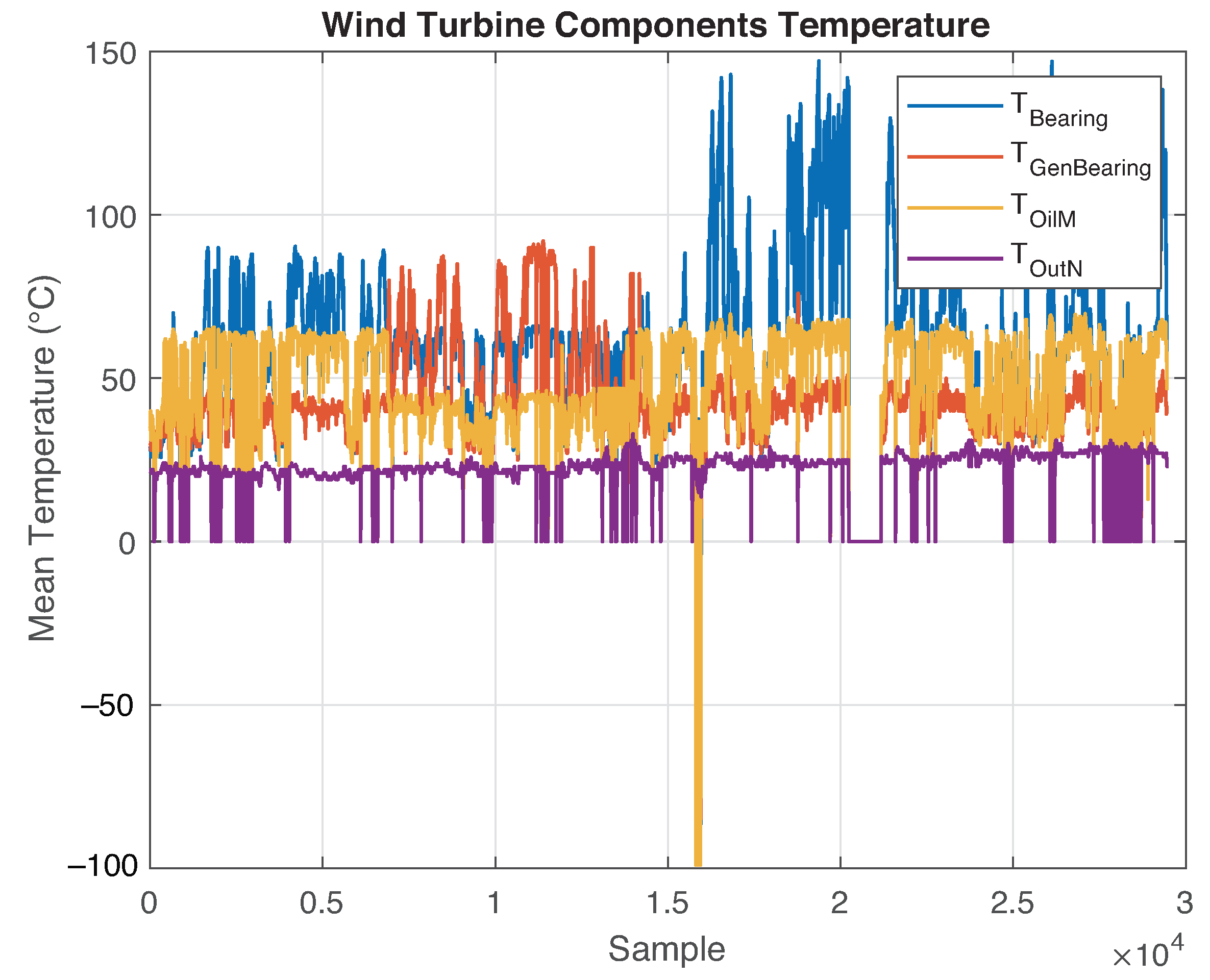
- File 1: This file contains the monitoring data of the SCADA system corresponding to WT number 15 of the farm, as measured between 1 January 2015 and 1 August 2015. The file comprises 29,489 rows and 20 columns, where each recorded measurement corresponds to the mean value of all data monitored for 10 min (slow rate SCADA data). The first column contains the exact date and time of the measurement; the remaining columns contain the data of different monitored variables, which are listed in Table 1.
- File 2: This file is an alarm log that contains the time, date, description, and state of different alarms activated over the same period of file 1 for the same WT. It comprises 21 rows and 5 columns. The features that describe the alarm states are listed in Table 2.

| Index | Variable | Description | Units | Type |
|---|---|---|---|---|
| 0 | date_time | Date and time of the sample | - | timestamp |
| 1 | power | Generated real power | kW | Real |
| 2 | bearing_temp | Bearing temperature of the turbine | °C | Real |
| 3 | cos_phi | Power factor | - | Real |
| 4 | gen_1_speed | Speed of the generator | m/s | Real |
| 5 | gen_bearing_temp | Bearing temperature of the generator | °C | Real |
| 6 | grid_current | Grid current | A | Real |
| 7 | grid_fre | Grid frequency | Hz | Real |
| 8 | grid_v | Grid voltage | V | Real |
| 9 | int_fase_r | R-Phase intensity | A | Real |
| 10 | int_fase_s | S-Phase intensity | A | Real |
| 11 | int_fase_t | T-Phase intensity | A | Real |
| 12 | reac_power_gen | Generated reactive power | kVAR | Real |
| 13 | rotor_speed | Rotor speed | m/s | Real |
| 14 | setpoint_power_act | Power generation set point | kW | Real |
| 15 | temp_oil_mult | Oil temperature of the gearbox | °C | Real |
| 16 | temp_out_nacelle | External temperature of the turbine nacelle | °C | Real |
| 17 | v_fase_r | R-phase voltage | V | Real |
| 18 | v_fase_s | S-phase voltage | V | Real |
| 19 | v_fase_t | T-phase voltage | V | Real |
| 20 | wind | Wind speed | m/s | Real |
| Variable | Description | Type |
|---|---|---|
| date_time | Date and time of the alarm | timestamp |
| model | Model of the wind turbine (wind turbine number inside the park) | String |
| code_desc | Description and code of the fault | String |
| status | Status of the alarm (ON, OFF) | Bool |
| alarm | Alarm active or not (0,1) | Bool |
3. Fault Detection Methodology
3.1. Data Analysis, Preprocessing and Labeling
3.2. Data Modeling and Dimension Reduction by Principal Component Analysis
3.3. Techniques for Dealing with Imbalanced Data
3.3.1. Random Oversampling
3.3.2. Data Reshaping
- Step 1. Each feature of the dataset described in Equation (1) is divided into small pieces of data called windows , where represents the floor function. All windows must contain the same number of observations. The number of observations captured by each window is called the window size , which determines the amount of data captured. Therefore, it must be selected carefully; if a large amount of data are captured, then important patterns of the dataset may be removed when these are grouped over a single new sample. In contrast, if insufficient data are captured, then the method will be ineffective because the new sample will not be sufficiently rich to enhance the process. To avoid these drawbacks, was carefully selected by considering the characteristics of the dataset such as sampling time, amount of data, and physical variable behavior. All data are collected such that, if the dataset is time-dependent, it will not mix any observations to maintain its time-dependence and avoid data leakage.
- Step 2. All information inside the window , of size is captured and stored as a new observation. All windows that contain at least one faulty observation are relabeled as faulty.
- Step 3. Each new observation is stacked to create a new feature matrix with dimensions .
- Step 4. After reshaping the data, it can be split into training and testing sets to be standardized and used to train and test the models.
3.4. Machine Learning Classifiers
3.4.1. k Nearest Neighbors (kNN)
3.4.2. Support Vector Machines (SVM)
3.4.3. Random under Sampling Boost (RUSBoost)
3.4.4. Performance Measures for Machine Learning Classifiers
- Accuracy (). Measures the number of correct predictions made by the model over the total number of observations.
- Precision or positive predictive value (). Measures the number of correctly classified positive class labels over the total number of positive-predicted labels, and it describes the proportion of correctly predicted positive observations.
- False discovery rate (). Measures the number of incorrectly classified positive class labels over the total number of positive predicted labels, describes the proportion of incorrectly predicted positive observations, and complements the information obtained by the precision.
- Negative predictive value (). Measures the number of correctly classified negative-class labels over the total number of negative predicted labels, and it describes the proportion of correctly predicted negative observations.
- False omission rate (). Measures the number of incorrectly classified negative-class labels over the total number of negative predicted labels, describes the proportion of incorrectly predicted negative observations, and it is complementary to the negative predictive value.
- Sensitivity/Recall/True positive rate (). Describes the fraction of correctly classified positive observations.
- F1 score (). It is the harmonic mean between precision and recall. It is calculated using
- Specificity/False positive rate (). The harmonic mean between precision and recall.
3.5. Experimental Framework
- Test 1. The dataset was split at an observation labeled as faulty. That observation was strategically selected to ensure that the resulting subsets have sufficient healthy and faulty information for the training and testing processes. Another reason to split the dataset this way is to maintain its time-dependence and eliminate the risk of data leakage. Therefore, this approach is called the time split. Afterwards, the data are standardized and modeled with the PCA method. The RUSBoost algorithm was fed with these data without any further processing to create a performance baseline. Then, the training and testing datasets used to feed the kNN and SVM algorithms were oversampled to create a balance using or , depending on which one is the minority class. This method is illustrated in Figure 10.
- Test 2. The time series dataset was reshaped as detailed in Section 3.3.2. The new observations with faults were identified, and the observations were modeled using the PCA method. Then, the data were split using the method described in test 1 (time split). The RUSBoost algorithm was fed with reshaped data without any further processing to obtain the performance baseline. The training and testing datasets used to feed the kNN and SVM algorithms were oversampled; the oversampling method became necessary as the data imbalance was worsened by reshaping. The balance is generated using or , depending on which is the minority class.
- k-nearest neighbors. In this algorithm, the number of nearest neighbors swept is between 1 and 200, and the Euclidean distance is used.
- SVM. The SVM is configured to function as a nonlinear separator using the radial basis function. It is tuned using the kernel scale (commonly known as the gamma factor) and a box constraint C (also known as the C factor or weighting factor) for the misclassified data. To test soft and hard classification boundaries, the hyperparameters were changed from small to large values. The number of PCs () selected for each dataset was considered to tune the kernel scale. Furthermore, the kernel scale was computed as the weighted square root of the number of PCs of the dataset used.
- RUSBoost. The hyperparameters of this algorithm are the maximum splits of the tree , the number of learning cycles , or iterations where the algorithm is going to run to select the best tree by majority voting. The learning rate that controls the shrinkage of the contribution of each new base model added to the series via gradient boosting is
4. Results
4.1. Test 1: Time Split
4.1.1. kNN Results
4.1.2. SVM Results
4.1.3. RUSBoost Results
4.1.4. Performance Charts
4.2. Test 2: Data Reshaping
4.2.1. kNN Results
4.2.2. SVM Results
4.2.3. RUSBoost Results
4.2.4. Performance Charts
5. Discussion
6. Conclusions
Author Contributions
Funding
Institutional Review Board Statement
Informed Consent Statement
Data Availability Statement
Acknowledgments
Conflicts of Interest
Abbreviations
| Accuracy | |
| CPVE | Cumulative proportion of variance explained |
| score | |
| False discovery rate | |
| False negative | |
| False omission rate | |
| False positive | |
| False positive rate | |
| kNN | k-nearest neighbors |
| Negative predictive value | |
| Obs | Observations |
| OS | Operating system |
| PC | Principal component |
| PCA | Principal component analysis |
| Positive predictive value | |
| PVE | Proportion of variance explained |
| RUSBoost | Random under sampling boost |
| SCADA | Supervisory control and data acquisition |
| SVM | Support vector machine |
| True negative | |
| True positive | |
| True positive rate | |
| WT | Wind turbine |
References
- Wang, S.; Yang, H.; Pham, Q.B.; Khoi, D.N.; Nhi, P.T.T. An Ensemble Framework to Investigate Wind Energy Sustainability Considering Climate Change Impacts. Sustainability 2020, 12, 876. [Google Scholar] [CrossRef] [Green Version]
- Rosales-Asensio, E.; Borge-Diez, D.; Blanes-Peiró, J.J.; Pérez-Hoyos, A.; Comenar-Santos, A. Review of wind energy technology and associated market and economic conditions in Spain. Renew. Sustain. Energy Rev. 2019, 101, 415–427. [Google Scholar] [CrossRef]
- Wind Energy in Spain. Available online: https://www.aeeolica.org/en/about-wind-energy/wind-energy-in-spain/ (accessed on 1 February 2021).
- Rodríguez, X.A.; Regueiro, R.M.; Doldán, X.R. Analysis of productivity in the Spanish wind industry. Renew. Sustain. Energy Rev. 2020, 118, 109573. [Google Scholar] [CrossRef]
- Spain Hits 44.7% Renewables Share in 7-mo 2020. Available online: https://renewablesnow.com/news/spain-hits-447-renewables-share-in-7-mo-2020-708939/ (accessed on 3 February 2021).
- Shafiee, M.; Sørensen, J.D. Maintenance optimization and inspection planning of wind energy assets: Models, methods and strategies. Reliab. Eng. Syst. Saf. 2019, 192, 105993. [Google Scholar] [CrossRef]
- Lin, J.; Pulido, J.; Asplund, M. Reliability analysis for preventive maintenance based on classical and Bayesian semi-parametric degradation approaches using locomotive wheel-sets as a case study. Reliab. Eng. Syst. Saf. 2015, 134, 143–156. [Google Scholar] [CrossRef] [Green Version]
- Florescu, A.; Barabas, S.; Dobrescu, T. Research on Increasing the Performance of Wind Power Plants for Sustainable Development. Sustainability 2019, 11, 1266. [Google Scholar] [CrossRef] [Green Version]
- Krishna, D.G. Preventive maintenance of wind turbines using Remote Instrument Monitoring System. In Proceedings of the 2012 IEEE Fifth Power India Conference, Murthal, India, 19–22 December 2012; pp. 1–4. [Google Scholar]
- Mazidi, P.; Du, M.; Tjernberg, L.B.; Bobi, M.A.S. A performance and maintenance evaluation framework for wind turbines. In Proceedings of the 2016 International Conference on Probabilistic Methods Applied to Power Systems (PMAPS), Beijing, China, 16–20 October 2016; pp. 1–8. [Google Scholar]
- Sequeira, C.; Pacheco, A.; Galego, P.; Gorbeña, E. Analysis of the efficiency of wind turbine gearboxes using the temperature variable. Renew. Energy 2019, 135, 465–472. [Google Scholar] [CrossRef]
- Lebranchu, A.; Charbonnier, S.; Bérenguer, C.; Prévost, F. A combined mono- and multi-turbine approach for fault indicator synthesis and wind turbine monitoring using SCADA data. ISA Trans. 2019, 87, 272–281. [Google Scholar] [CrossRef]
- Wang, K.S.; Sharma, V.S.; Zhang, Z.Y. SCADA data based condition monitoring of wind turbines. Adv. Manuf. 2014, 2, 61–69. [Google Scholar] [CrossRef] [Green Version]
- Kusiak, A.; Verma, A. Analyzing bearing faults in wind turbines: A data-mining approach. Renew. Energy 2012, 48, 110–116. [Google Scholar] [CrossRef]
- Dao, P.B.; Staszewski, W.J.; Barszcz, T.; Uhl, T. Condition monitoring and fault detection in wind turbines based on cointegration analysis of SCADA data. Renew. Energy 2018, 116, 107–122. [Google Scholar] [CrossRef]
- Alvarez, E.J.; Ribaric, A.P. An improved-accuracy method for fatigue load analysis of wind turbine gearbox based on SCADA. Renew. Energy 2018, 115, 391–399. [Google Scholar] [CrossRef]
- Rodríguez-López, M.A.; López-González, L.M.; López-Ochoa, L.M.; Las-Heras-Casas, J. Development of indicators for the detection of equipment malfunctions and degradation estimation based on digital signals (alarms and events) from operation SCADA. Renew. Energy 2016, 99, 224–236. [Google Scholar] [CrossRef]
- Qiu, Y.; Feng, Y.; Infield, D. Fault diagnosis of wind turbine with SCADA alarms based multidimensional information processing method. Renew. Energy 2020, 145, 1923–1931. [Google Scholar] [CrossRef]
- Dai, J.; Yang, W.; Cao, J.; Liu, D.; Long, X. Ageing assessment of a wind turbine over time by interpreting wind farm SCADA data. Renew. Energy 2018, 116, 199–208. [Google Scholar] [CrossRef] [Green Version]
- Ruiming, F.; Minling, W.; Xinhua, G.; Rongyan, S.; Pengfei, S. Identifying early defects of wind turbine based on SCADA data and dynamical network marker. Renew. Energy 2020, 154, 625–635. [Google Scholar] [CrossRef]
- Jha, S.K.; Bilalovic, J.; Jha, A.; Patel, N.; Zhang, H. Renewable energy: Present research and future scope of Artificial Intelligence. Renew. Sustain. Energy Rev. 2017, 77, 297–317. [Google Scholar] [CrossRef]
- Pozo, F.; Vidal, Y.; Serrahima, J.M. On real-time fault detection in wind turbines: Sensor selection algorithm and detection time reduction analysis. Energies 2016, 9, 520. [Google Scholar] [CrossRef] [Green Version]
- Bangalore, P.; Patriksson, M. Analysis of SCADA data for early fault detection, with application to the maintenance management of wind turbines. Renew. Energy 2018, 115, 521–532. [Google Scholar] [CrossRef]
- Zhao, H.; Liu, H.; Hu, W.; Yan, X. Anomaly detection and fault analysis of wind turbine components based on deep learning network. Renew. Energy 2018, 127, 825–834. [Google Scholar] [CrossRef]
- Kong, Z.; Tang, B.; Deng, L.; Liu, W.; Han, Y. Condition monitoring of wind turbines based on spatio-temporal fusion of SCADA data by convolutional neural networks and gated recurrent units. Renew. Energy 2020, 146, 760–768. [Google Scholar] [CrossRef]
- Helbing, G.; Ritter, M. Deep Learning for fault detection in wind turbines. Renew. Sustain. Energy Rev. 2018, 98, 189–198. [Google Scholar] [CrossRef]
- Imbalanced Data. Available online: https://developers.google.com/machine-learning/data-prep/construct/sampling-splitting/imbalanced-data (accessed on 11 March 2021).
- Castellani, F.; Garibaldi, L.; Daga, A.P.; Astolfi, D.; Natili, F. Diagnosis of faulty wind turbine bearings using tower vibration measurements. Energies 2020, 13, 1474. [Google Scholar] [CrossRef] [Green Version]
- Wang, Y.; Ma, X.; Qian, P. Wind turbine fault detection and identification through PCA-based optimal variable selection. IEEE Trans. Sustain. Energy 2018, 9, 1627–1635. [Google Scholar] [CrossRef] [Green Version]
- Zhao, Y.; Li, D.; Dong, A.; Kang, D.; Lv, Q.; Shang, L. Fault prediction and diagnosis of wind turbine generators using SCADA data. Energies 2017, 10, 1210. [Google Scholar] [CrossRef] [Green Version]
- Pozo, F.; Vidal, Y. Wind turbine fault detection through principal component analysis and statistical hypothesis testing. Energies 2016, 9, 3. [Google Scholar] [CrossRef] [Green Version]
- Pozo, F.; Vidal, Y.; Salgado, Ó. Wind turbine condition monitoring strategy through multiway PCA and multivariate inference. Energies 2018, 11, 749. [Google Scholar] [CrossRef] [Green Version]
- Fleckestein, J.E. Three-Phase Electrical Power; CRC Press: Boca Raton, FL, USA, 2016. [Google Scholar]
- Jolliffe, I.T. Principal Component Analysis; Springer: Berlin/Heidelberg, Germany, 2002. [Google Scholar]
- Mohammed, R.; Rawashdeh, J.; Abdullah, M. Machine Learning with Oversampling and Undersampling Techniques: Overview Study and Experimental Results. In Proceedings of the 2020 11th International Conference on Information and Communication Systems (ICICS), Irbid, Jordan, 7–9 April 2020; pp. 243–248. [Google Scholar]
- Pang, Y.; Chen, Z.; Peng, L.; Ma, K.; Zhao, C.; Ji, K. A Signature-Based Assistant Random Oversampling Method for Malware Detection. In Proceedings of the 2019 18th IEEE International Conference On Trust, Security and Privacy in Computing and Communications/13th IEEE International Conference on Big Data Science and Engineering (TrustCom/BigDataSE), Rotorua, New Zealand, 5–8 August 2019; pp. 256–263. [Google Scholar]
- Ghazikhani, A.; Yazdi, H.S.; Monsefi, R. Class imbalance handling using wrapper-based random oversampling. In Proceedings of the 20th Iranian Conference on Electrical Engineering (ICEE2012), Tehran, Iran, 15–17 May 2012; pp. 611–616. [Google Scholar]
- Puruncajas, B.; Vidal, Y.; Tutivén, C. Vibration-Response-Only Structural Health Monitoring for Offshore Wind Turbine Jacket Foundations via Convolutional Neural Networks. Sensors 2020, 20, 3429. [Google Scholar] [CrossRef] [PubMed]
- Ruiz, M.; Mujica, L.E.; Alferez, S.; Acho, L.; Tutiven, C.; Vidal, Y.; Rodellar, J.; Pozo, F. Wind turbine fault detection and classification by means of image texture analysis. Mech. Syst. Signal Process. 2018, 107, 149–167. [Google Scholar] [CrossRef] [Green Version]
- Ghosh, S.; Das, N.; Nasipuri, M. Reshaping inputs for convolutional neural network: Some common and uncommon methods. Pattern Recognit. 2019, 93, 79–94. [Google Scholar] [CrossRef]
- Janssen, L.A.L.; Lopez Arteaga, I. Data processing and augmentation of acoustic array signals for fault detection with machine learning. J. Sound Vib. 2020, 483, 115483. [Google Scholar] [CrossRef]
- Huang, Z.; Zhu, J.; Lei, J.; Li, X.; Tian, F. Tool Wear Predicting Based on Multisensory Raw Signals Fusion by Reshaped Time Series Convolutional Neural Network in Manufacturing. IEEE Access 2019, 7, 178640–178651. [Google Scholar] [CrossRef]
- Fernandez, A.; Garcia, S.; Herrera, F.; Chawla, N.V. SMOTE for Learning from Imbalanced Data: Progress and Challenges, Marking the 15-year Anniversary. J. Artif. Intell. Res. 2018, 61, 863–905. [Google Scholar] [CrossRef]
- Batista, G.E.A.P.A.; Prati, R.C.; Monard, M.C. A study of the behavior of several methods for balancing machine learning training data. ACM SIGKDD Explor. Newsl. 2004, 6, 20–29. [Google Scholar] [CrossRef]
- Guido, S.; Muller, A. Introduction to Machine Learning with Python; O’Reilly UK Ltd.: Farnham, UK, 2016. [Google Scholar]
- Russel, S.; Norvig, P. Artificial Intelligence: A Modern Approach, 3rd ed.; Prentice Hall: Upper Saddle River, NJ, USA, 2010. [Google Scholar]
- Géron, A. Hands-On Machine Learning with Scikit-Learn and TensorFlow: Concepts, Tools, and Techniques to Build Intelligent Systems; O’Reilly Media: Sebastopol, CA, USA, 2017. [Google Scholar]
- Seiffert, C.; Khoshgoftaar, T.M.; Hulse, J.V.; Napolitano, A. RUSBoost: A Hybrid Approach to Alleviating Class Imbalance. IEEE Trans. Syst. Man Cybern. Part A Syst. Humans 2010, 40, 185–197. [Google Scholar] [CrossRef]
- Sokolova, M.; Lapalme, G. A systematic analysis of performance measures for classification tasks. Inf. Process. Manag. 2009, 45, 427–437. [Google Scholar] [CrossRef]


| Alarm | Code | Description |
|---|---|---|
| TRA-137 Sobre-tmp | 137 | over-temperature |
| TRA-135 Sobre-tmp | 135 | over-temperature |
| TRA-137 Alta tmp | 137 | high temperature |
| TRA-135 Alta tmp | 135 | high temperature |
| Predicted Class | |||
|---|---|---|---|
| Negative | Positive | ||
| True class | Negative | True negative () a | False positive () a |
| Positive | False negative () a | True positive () a | |
| Test | Approach | Window Size (Hours) | Window Size (Obs) | PCs | Training Size (Obs) | Training Faults (Obs) | Validation Size (Obs) | Validation Faults (Obs) |
|---|---|---|---|---|---|---|---|---|
| 1 | Time Split | − | − | 6 | 28,895 | 18 | 593 | 11 |
| 2 | Reshaping | 0.5 | 3 | 10 | 9632 | 8 | 197 | 4 |
| 1 | 6 | 16 | 4816 | 5 | 98 | 2 | ||
| 3 | 18 | 31 | 1601 | 2 | 37 | 2 |
| Test | Approach | Window Size (Hours) | Window Size (Obs) | PCs | Training Size (Obs) | Training Faults (Obs) | Validation Size (Obs) | Validation Faults (Obs) |
|---|---|---|---|---|---|---|---|---|
| 1 | Time Split | − | − | 6 | 57,731 | 28,854 | 1143 | 561 |
| 2 | Reshaping | 0.5 | 3 | 10 | 19,240 | 9616 | 381 | 188 |
| 1 | 6 | 16 | 9616 | 4805 | 190 | 94 | ||
| 3 | 18 | 31 | 3195 | 1696 | 67 | 32 |
| Data Set | Box Constraint | Kernel Scale |
|---|---|---|
| non-oversampled | 50 | 0.40 |
| oversampled | 1000 | 14.69 |
| Dataset | Maximum Splits | Learning Cycles |
|---|---|---|
| non-oversampled | 5 | 1500 |
| Algorithm | Data Set | (%) | (%) | (%) | (%) | (%) |
|---|---|---|---|---|---|---|
| kNN | non-oversampled | 98.65 | 100.00 | 27.27 | 42.85 | 100.00 |
| oversampled | 96.93 | 94.12 | 100.00 | 96.97 | 93.98 | |
| SVM | non-oversampled | 99.15 | 100.00 | 54.54 | 70.58 | 100.00 |
| oversampled | 95.36 | 91.50 | 99.82 | 95.48 | 91.06 | |
| RUSBoost | non-oversampled | 93.59 | 22.44 | 100.00 | 36.66 | 93.47 |
| Algorithm | Data Set | Training Time (s) | Prediction Time (s) |
|---|---|---|---|
| kNN | non-oversampled | 9.78 × | 2.31 × |
| oversampled | 1.17 × | 3.61 × | |
| SVM | non-oversampled | 5.97 × | 5.60 × |
| oversampled | 1.98 | 1.75 × | |
| RUSBoost | non-oversampled | 15.64 | 7.78 × |
| Window Size/Data Set | Nonoversampled | Oversampled |
|---|---|---|
| 30 min | 1 | 90 |
| 1 h | 1 | 4 |
| 3 h | 1 | 17 |
| Nonoversampled | Oversampled | |||
|---|---|---|---|---|
| Window Size | Box Constraint | Kernel Scale | Box Constraint | Kernel Scale |
| 30 min | 5 | 1.58 | 1 | 18.97 |
| 1 h | 50 | 8.00 | 1 | 8.00 |
| 3 h | 1 | 0.92 | 1 | 55.67 |
| Window Size | Maximum Splits | Learning Cycles |
|---|---|---|
| 30 min | 1 | 5000 |
| 1 h | 1 | 1500 |
| 3 h | 5 | 25 |
| Algorithm | Windows Size | Data Set | (%) | (%) | (%) | (%) | (%) |
|---|---|---|---|---|---|---|---|
| kNN | h | non-oversampled | 98.98 | 100.00 | 50.00 | 66.66 | 100.00 |
| h | oversampled | 92.65 | 87.38 | 99.46 | 93.03 | 86.01 | |
| SVM | h | non-oversampled | 98.98 | 100.00 | 50.00 | 66.66 | 100.00 |
| h | oversampled | 75.59 | 66.90 | 100.00 | 80.17 | 51.81 | |
| RUSBoost | h | non-oversampled | 88.32 | 14.81 | 100.00 | 25.80 | 88.08 |
| kNN | 1 h | non-oversampled | 95.92 | 25.00 | 50.00 | 33.33 | 96.87 |
| 1 h | oversampled | 97.37 | 94.95 | 100.00 | 97.41 | 94.79 | |
| SVM | 1 h | non-oversampled | 100.00 | 100.00 | 100.00 | 100.00 | 100.00 |
| 1 h | oversampled | 94.73 | 90.38 | 100.00 | 94.94 | 89.58 | |
| RUSBoost | 1 h | non-oversampled | 76.53 | 8.00 | 100.00 | 14.81 | 76.04 |
| kNN | 3 h | non-oversampled | 94.59 | 0.00 | 0.00 | 0.00 | 100.00 |
| 3 h | oversampled | 74.62 | 94.11 | 50.00 | 65.30 | 97.14 | |
| SVM | 3 h | non-oversampled | 94.59 | 0.00 | 0.00 | 0.00 | 100.00 |
| 3 h | oversampled | 70.14 | 80.00 | 50.00 | 61.53 | 88.57 | |
| RUSBoost | 3 h | non-oversampled | 83.78 | 25.00 | 100.00 | 40.00 | 82.85 |
| Algorithm | Windows Size | Data Set | Training Time (s) | Prediction Time (s) |
|---|---|---|---|---|
| kNN | h | non-oversampled | ||
| h | oversampled | 6.51 × | 1.68 × | |
| SVM | h | non-oversampled | 2.01 × | 4.41 × |
| h | oversampled | 2.32 | 9.05 × | |
| RUSBoost | h | non-oversampled | 31.83 | 2.24 |
| kNN | 1 h | non-oversampled | 2.67 × | 5.21 × |
| 1 h | oversampled | 2.79 × | 5.00 × | |
| SVM | 1 h | non-oversampled | 6.72 × | 4.52 × |
| 1 h | oversampled | 3.31 × | 5.71 × | |
| RUSBoost | 1 h | non-oversampled | 7.68 | 5.73 × |
| kNN | 3 h | non-oversampled | 5.17 × | 5.87 × |
| 3 h | oversampled | 7.33 × | 1.27 × | |
| SVM | 3 h | non-oversampled | 3.32 × | 1.37 × |
| 3 h | oversampled | 4.75 × | 5.42 × | |
| RUSBoost | 3 h | non-oversampled | 1.18 × | 9.94 × |
Publisher’s Note: MDPI stays neutral with regard to jurisdictional claims in published maps and institutional affiliations. |
© 2021 by the authors. Licensee MDPI, Basel, Switzerland. This article is an open access article distributed under the terms and conditions of the Creative Commons Attribution (CC BY) license (http://creativecommons.org/licenses/by/4.0/).
Share and Cite
Velandia-Cardenas, C.; Vidal, Y.; Pozo, F. Wind Turbine Fault Detection Using Highly Imbalanced Real SCADA Data. Energies 2021, 14, 1728. https://doi.org/10.3390/en14061728
Velandia-Cardenas C, Vidal Y, Pozo F. Wind Turbine Fault Detection Using Highly Imbalanced Real SCADA Data. Energies. 2021; 14(6):1728. https://doi.org/10.3390/en14061728
Chicago/Turabian StyleVelandia-Cardenas, Cristian, Yolanda Vidal, and Francesc Pozo. 2021. "Wind Turbine Fault Detection Using Highly Imbalanced Real SCADA Data" Energies 14, no. 6: 1728. https://doi.org/10.3390/en14061728