Analysis and Pareto Frontier Based Tradeoff Design of an Integrated Magnetic Structure for a CLLC Resonant Converter

Abstract

This paper proposes an integrated magnetic structure for a CLLC resonant converter. With the proposed integrated magnetic structure, two resonant inductances and the transformer are integrated into one magnetic core, which improves the power density of the CLLC resonant converter. In the proposed integrated magnetic structure, two resonant inductances are decoupled with the transformer and can be adjusted by the number of turns in each inductance. Furthermore, two resonant inductances are coupled to reduce the number of turns in each inductance. As a result, the conduction loss can be reduced. The trade-off design of the integrated magnetic structure is carried out based on the Pareto optimization procedure. With the Pareto optimization procedure, both high efficiency and high-power density can be achieved. The proposed integrated magnetic structure is validated by theoretical analysis, simulations, and experiments.

1. Introduction

Bidirectional dc-dc converters are widely applied in the uninterrupted power supplies (UPS), electric vehicles, energy storage systems, smart grid power systems, fuel cells and supercapacitors hybrid systems [1,2,3,4] to achieve bidirectional power flows.

Of all the bidirectional dc-dc topologies, the CLLC resonant converter, which is shown in Figure 1, has become increasingly popular, due to its advantages of high efficiency, buck and boost capability, and bidirectional power transfer [5,6]. In addition, compared with the dual active bridge (DAB) converter, where the Zero-Voltage-Switching is lost under light load conditions, the CLLC resonant converter can operate under Zero-Voltage-Switching (ZVS) of the primary switches and Zero-Current-Switching (ZCS) of the secondary switches over the whole load range [5,6]. As a result, the switching loss can be greatly reduced. Due to the soft switching characteristics, the CLLC resonant converter can operate at a high frequency, which results in a high-power density. Furthermore, the voltage stress of the power switches in the CLLC resonant converter is confined to the input voltage and output voltage without any clamp circuit [5]. Therefore, the CLLC resonant converters have been investigated and reported extensively.

In the CLLC topology level, the working principles, equations of main parameters, synchronous rectifications, and the controls of CLLC resonant converters have been investigated [5,7,8,9]. The operation principles and the equations of the main parameters are well stated in [5,7,8]. To reduce the conduction loss, a novel synchronous rectification scheme based on small phase shift technique is proposed in [9].

In the component level, in order to improve the power density, the wide bandgap semiconductor devices, such as the Gallium Nitride (GaN) and Silicon Carbide (SiC) switches, have been utilized to reduce the power loss of the switches and increase the switching speed. However, with the reduction of the power loss of the switches, the magnetic design is still very challenging mainly due to the number of the magnetic cores in the CLLC resonant converter, where two resonant inductances and a transformer are required [10,11,12].

The most basic way to build two resonant inductances and a transformer for a CLLC resonant converter is to use three detached magnetic cores, with two magnetic cores for the resonant inductances and another for the transformer, which is shown in Figure 2a [5,9]. The advantage of the basic way is that the two resonant inductances can be adjusted independently based on the optimal design of the CLLC resonant converter. However, the application of the detached magnetic cores will lead to the large volume of the converter, which will reduce the power density.

The conventional integrated magnetic structure as shown in Figure 2b, where the leakage inductances of the transformer are used as the resonant inductances, is applied in the CLLC resonant converter to increase the power density [12,13,14]. The leakage energy is stored between the primary winding and the secondary winding. The leakage inductance (L_r) can be adjusted by the distance of the primary winding and secondary winding (d_w), while the magnetizing inductance (L_m) is adjusted by the thickness of the air gap (d_a). With this magnetic integration method, only one magnetic core is required. However, the shortcomings of this magnetic structure are summarized as follows:

Firstly, the extra distance (d_w) is required to achieve the desired resonant inductances, which will increase the volume of the magnetic core and the corresponding core loss.

Secondly, due to the high leakage flux between primary and secondary winding, the conductors will suffer more severe proximity effect, which will increase the copper loss.

Finally, it should be noted that the range of the leakage inductances is limited by the height of the magnetic core (h_c), which means the desired resonant inductances may not be achieved when large resonant inductances are required.

In order to solve the above problems, an integrated magnetic structure is proposed for the CLLC resonant converter, which is illustrated in Figure 2c. In the proposed integrated magnetic structure, instead of using the leakage inductances as the resonant inductances, two extra inductances, L_r1 and L_r2 are introduced to the magnetic core, which are coupled with each other but decoupled with L_m. The sums of the self-inductance (L_r1, L_r2) and the mutual inductance (M₁₂) are used as the resonant inductances (L_rp, L_rs). In addition, L_rp and L_rs can be adjusted by the number of turns (N_r1 and N_r2) and the air gap in the side legs (d_s) while L_m can be adjusted by the number of turns (N_p) and the air gap in the central leg (d_c). The advantages of the proposed integrated magnetic structure are summarized as follows:

Firstly, only one magnetic core is required, which is the same with the conventional integrated magnetic structure shown in Figure 2b.

Secondly, compared with Figure 2b, d_w is not required anymore and the volume of the magnetic core will be reduced. The proximity effect in Figure 2b will be reduced as well.

Thirdly, the resonant inductances can be easily increased by adding more turns for L_r1 and L_r2, so the range of the resonant inductances is expanded. As a result, the optimal design of the CLLC resonant converter can be achieved although large resonant inductances are required.

Finally, L_r1 and L_r2 are positively coupled to enhance the resonant inductances. As a result, the number of turns (N_r1 and N_r2) is reduced compared with using uncoupled inductances. As a result, the copper loss is reduced as well.

However, it is important to point out that in the proposed integrated magnetic structure, due to the positive coupling between L_r1 and L_r2, the magnetic flux density in the side legs will increase, which will result in more core loss. By increasing the cross-sectional area, both the magnetic flux density and the core loss will decrease. However, the core volume will increase. As a result, the core loss and the core volume always contradict each other. In order to further optimize the proposed integrated magnetic structure, with full consideration of the width of the central leg, w_c, the width of the side legs, w_s, and the depth of the magnetic core, w_d, the tradeoff design between the core volume and core loss is also investigated, which is based on the multi-objective optimization method, the Pareto optimization procedure. With the Pareto optimization procedure, the optimal design of the proposed integrated magnetic structure can be easily carried out for a specific application.

The rest of this paper is arranged as follows. The conventional integrated magnetic structure for the CLLC resonant converter is reviewed in Section 2. In Section 3, the operation principles and the analysis of the proposed integrated magnetic structure are elaborated and the equations of L_rp, L_rs and L_m are derived. In Section 4, the Pareto Frontier based multi-objective optimization of the proposed integrated magnetic structure is also investigated. In Section 5, the proposed magnetic structure and the multi-objective optimization are validated by the simulations and experiments. Section 6 contains a brief conclusion.

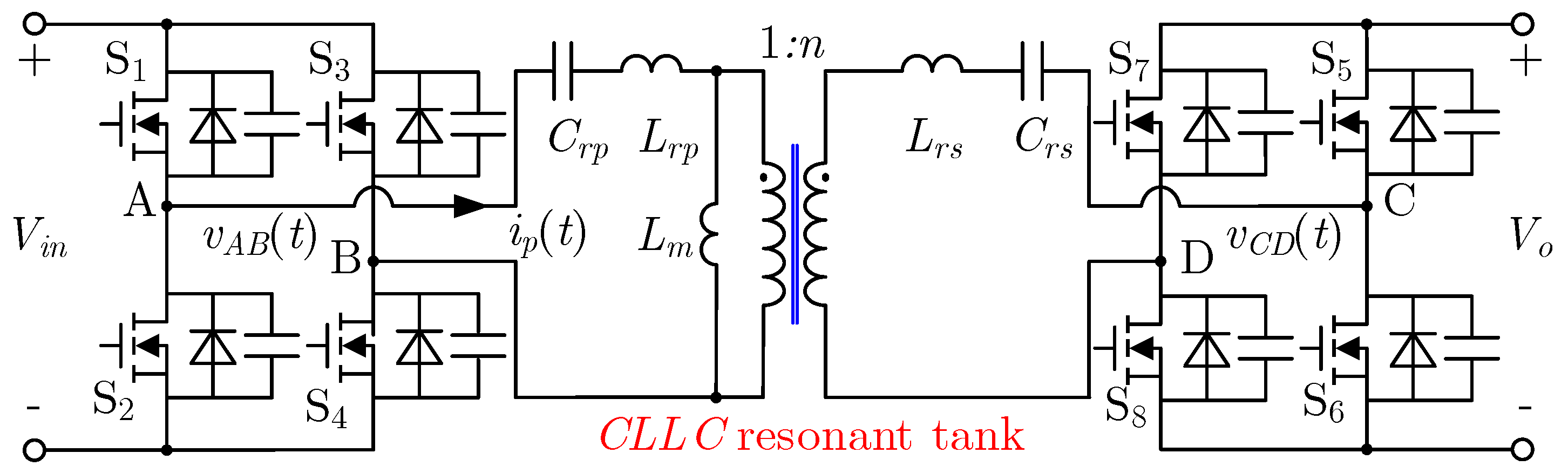
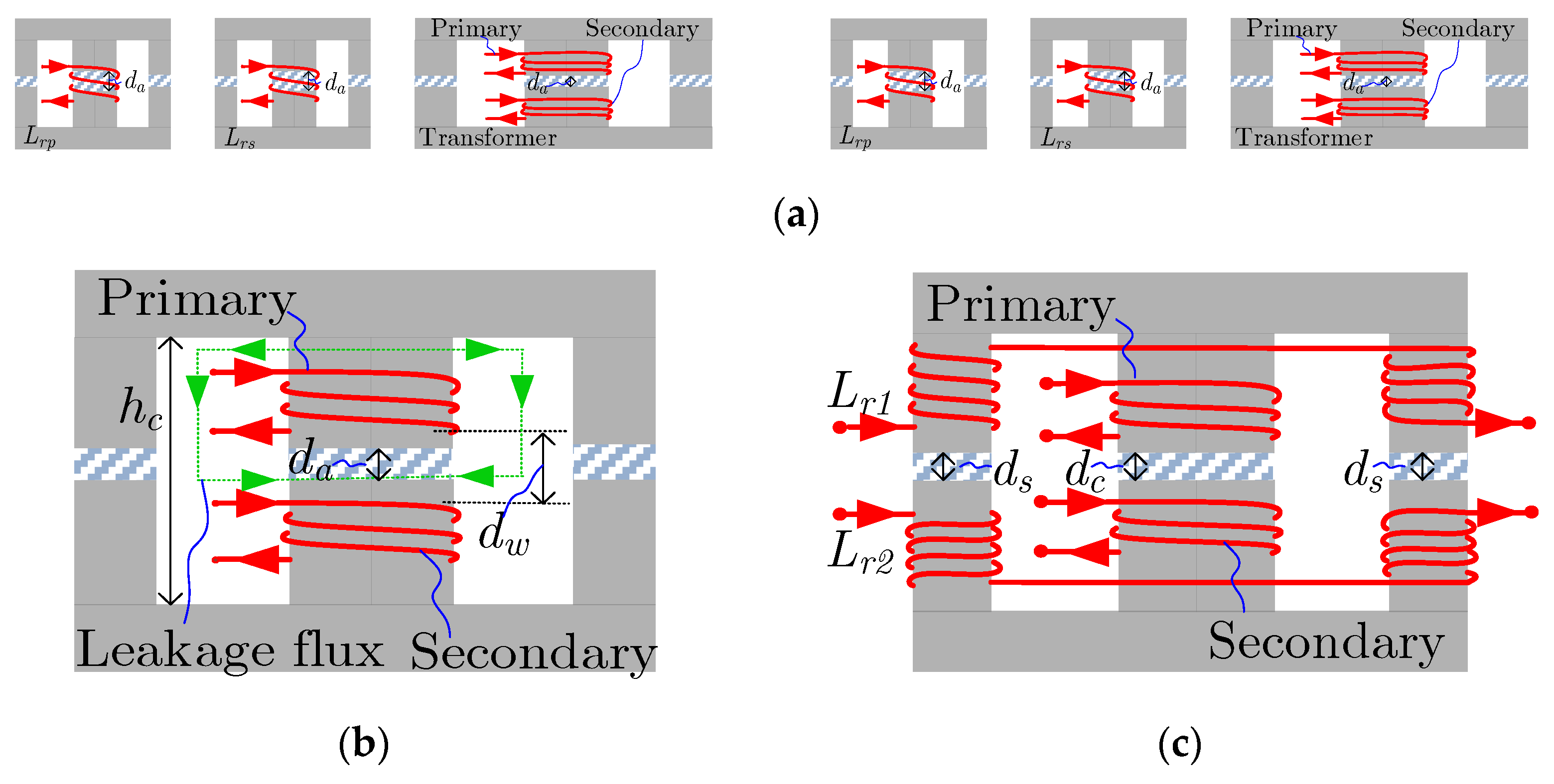
2. Review of the Conventional Method of Magnetic Integration in the CLLC Resonant Converter: Using the Leakage Inductances as the Resonant Inductances

The conventional integrated magnetic structure in a CLLC resonant converter is to use the leakage inductances as the resonant inductances, as shown in Figure 2b [12,13,14]. In this section, this conventional method is reviewed. The general equation of the leakage inductance of this method is derived and the shortcomings of this method are analyzed.

As shown in Figure 3, in order to increase the power density by reducing the number of the magnetic components, the leakage inductances of the planar transformer are utilized as the resonant inductances. The desired leakage inductances (L_rp and L_rs) are achieved by changing the distance between the primary winding and the secondary winding (d_w).

The winding configuration of a planar transformer and its corresponding magneto-motive force (MMF) are shown in Figure 3. The primary winding has n_p turns, which are distributed in m_p layers while the secondary winding has n_s turns, which are distributed in m_s layers. The distance between the primary winding and the secondary winding is d_w, which is adjusted to achieve the optimal leakage inductances. The air gap (d_a) is added to achieve the desired magnetizing inductance (L_m).

Assuming the current excitation to the primary winding is i_p, based on the distribution of MMF in Figure 3, the magnetic energy stored in the window can be calculated by [15,16,17]:

$$E_m=\frac{{\mu }_0{\mu }_r{n}_p^2{i}_p^2{W}_d}{6W_w}\left[2m_p{d}_p+2m_s{d}_s+\frac{\left(m_p-1\right)\left(2m_p-1\right)d_i}{m_p}+\frac{\left(m_s-1\right)\left(2m_s-1\right)d_i}{m_s}+6d_w\right]$$

(1)

where W_d is the depth of the window, W_w is the width of the window, d_p and d_s are the thickness of the primary winding and secondary winding, respectively, and d_i is the thickness of the insulation.

According to the relation between leakage inductance and magnetic energy, leakage inductances can be calculated by:

$$L_{rp}=L_{rs}=\frac{{\mu }_0{\mu }_r{n}_p^2{W}_d}{6W_w}\left[2m_p{d}_p+2m_s{d}_s+\frac{\left(m_p-1\right)\left(2m_p-1\right)d_i}{m_p}+\frac{\left(m_s-1\right)\left(2m_s-1\right)d_i}{m_s}+6d_w\right]$$

(2)

It can be concluded from Equation (2) that the leakage inductances can be changed by d_w, which can be calculated by:

$$d_w=\frac{W_w{L}_{rp}}{{\mu }_0{\mu }_r{n}_p^2{W}_d}-\frac{m_p{d}_p}{3}-\frac{m_s{d}_s}{3}-\frac{\left(m_p-1\right)\left(2m_p-1\right)d_i}{6m_p}-\frac{\left(m_s-1\right)\left(2m_s-1\right)d_i}{6m_s}$$

(3)

However, it is important to note the shortcomings of this method, which are summarized as follows:

Firstly, with increased d_w, the volume of the magnetic core will increase as well, which will not only reduce the power density of the converter, but also cause extra core loss.

Secondly, in order to achieve the desired leakage inductances, plenty of leakage fluxes should be stored between the primary winding and the secondary winding. However, the stored leakage flux will aggravate the proximity effect, which will cause more copper loss.

Finally, it should be noted that d_w is limited by the height of the window. As a result, the range of the leakage inductances is also limited by the window.

3. Proposed Integrated Magnetic Structure for the CLLC Resonant Converters

In this section, an integrated magnetic structure is proposed for a CLLC resonant converter, where two resonant inductances and a transformer are integrated in a magnetic core. At first, the working principles and the equations are elaborated. After that, the proposed integrated magnetic structure is compared with the conventional integrated magnetic structure to further show the advantages of the proposed integrated magnetic structure.

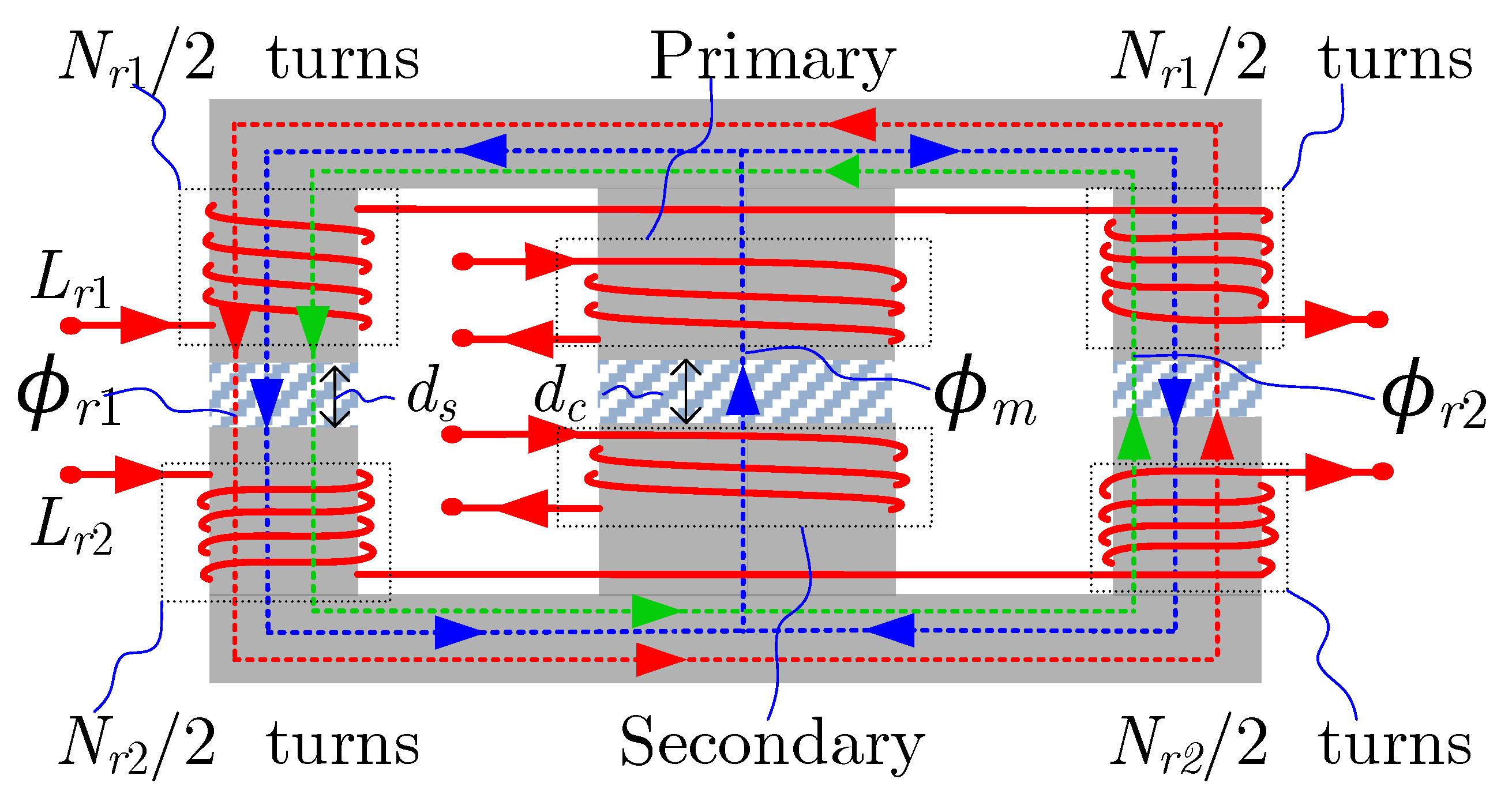
3.1. Proposed Integrated Magnetic Structure for the CLLC Resonant Converters

The proposed integrated magnetic structure and the corresponding magnetic flux are shown in Figure 4, where the primary winding and the secondary winding are wounded on the center leg while two extra inductances (L_r1 and L_r2) are wounded on the side legs. It is worthy to point out that the sums of the self-inductance (L_r1, L_r2) and the mutual inductance (M₁₂) are used as the resonant inductances (L_rp, L_rs).

The primary and secondary winding, which are wounded on the central leg, have N_p and N_s turns, respectively. The magnetic flux generated by L_m, ϕ_m, is shown by the blue dash line.

The inductance, L_r1, has N_r1 turns, with half of the turns are on the left leg while the other half are on the right leg. The way how the two halves are connected is shown in Figure 4. The flux generated by L_r1, ϕ_r1, is shown by the red dash line.

The inductance, L_r2, has N_r2 turns, with half of the turns are on the left leg while the other half are on the right leg. The way how the two halves are connected is shown in Figure 4. The flux generated by L_r2, ϕ_r2, is shown by the green dash line. The equivalent magnetic circuit with the excitation is shown in Figure 5.

Derivation of L_r1, L_r2, L_m, M_1m and M_2m

Neglecting the leakage flux, L_m, L_r1, L_r2, the mutual inductance between L_r1 and L_r2, M₁₂, the mutual inductance between L_r1 and L_m, M_1m and the mutual inductance between L_r2 and L_m, M_2m, will be derived as follows.

Assuming the current excitation of L_r1 is i_r1, the equivalent magnetic circuit is shown in Figure 5a.

Based on magnetic circuit analysis, the following equations can be derived:

$$\begin{gathered} R_c({\varphi }_{s1}+{\varphi }_{s2})+R_s{\varphi }_{s1}=-\frac{N_{r1}{i}_{r1}}{2} \\ {R}_c({\varphi }_{s1}+{\varphi }_{s2})+R_s{\varphi }_{s2}=\frac{N_{r1}{i}_{r1}}{2} \end{gathered}$$

(4)

where ϕ_s1, ϕ_s2 are the magnetic flux in the left-side leg and right-side leg, respectively. R_c and R_s are the magnetic reluctances of the central leg, side legs and yokes (including the air gaps).

According to Equation (4), ϕ_s1 and ϕ_s2 are:

$${\varphi }_{s1}=-\frac{i_{r1}{N}_{r1}}{2R_s}, {\varphi }_{s2}=\frac{i_{r1}{N}_{r1}}{2R_s}$$

(5)

According to the definitions of self-inductance and mutual inductance, with (5), L_r1, M_1m and M₁₂ can be calculated by:

$$L_{r1}=\frac{N_{r1}^2}{2R_s}, M_{1m}=0, M_{12}=\frac{N_{r1}{N}_{r2}}{2R_s}$$

(6)

As a result, L_m and L_r1 are decoupled.

Similarly, the current excitation of L_r2 is i_r2 and the equivalent magnetic circuit is shown in Figure 5b. Based on the magnetic circuit analysis, the following equations can be derived:

$$\begin{gathered} R_c({\varphi }_{s1}+{\varphi }_{s2})+R_s{\varphi }_{s1}=-\frac{N_{r2}{i}_{r2}}{2} \\ {R}_c({\varphi }_{s1}+{\varphi }_{s2})+R_s{\varphi }_{s2}=\frac{N_{r2}{i}_{r2}}{2} \end{gathered}$$

(7)

According to the definitions of self-inductance and mutual inductance, with (7), L_r2, M_2m and M₂₁ can be calculated by:

$$L_{r1}=\frac{N_{r2}^2}{2R_s}, M_{1m}=0, M_{21}=\frac{N_{r1}{N}_{r2}}{2R_s}$$

(8)

As a result, L_m and L_r2 are decoupled.

The current excitation of L_m is i_m and the equivalent magnetic circuit is shown in Figure 5c. L_m can be calculated by:

$$L_m=\frac{N_p^2}{2R_c+R_s}$$

(9)

Due to the coupling between L_r1 and L_r2, the actual resonant inductances, L_rp and L_rs are:

$$\begin{gathered} L_{rp}=\frac{N_{r1}(N_{r1}+N_{r2})}{2R_s} \\ {L}_{rs}=\frac{N_{r2}(N_{r1}+N_{r2})}{2R_s} \end{gathered}$$

(10)

3.2. Comparison with the Conventional Integrated Magnetic Structure for a CLLC Resonant Converter (Using the Leakage Inductances as the Resonant Inductances)

In this part, the proposed integrated magnetic structure is compared with the conventional integrated magnetic structure, where the leakage inductances are used as the resonant inductances. The parameters of the CLLC resonant converter are listed in

Table 1. Parameters of the CLLC resonant converter and the magnetic core.

Symbol	Values	Symbol	Values
Lrp	30 µH	Aes	519 mm2
Lrs	30 µH	Aec	1038 mm2
Lm	550 µH	Kc	1.8714
Np	16	α	0.8258
Ns	16	β	2.322

. The magnetic core selected for the CLLC resonant converter is ELP 64/10/50 with N87 from TDK. Two magnetic cores are used in parallel to increase the cross-sectional area. The parameters of the magnetic core are shown in Table 1 as well.

In order to make a fair comparison, the two integrated magnetic structures share the same winding configuration, where primary winding is distributed into 4 layers, with each layer consisting of 4 turns. In order to achieve the desired L_m, the thickness of the air gap, d_a, is set as 0.14 mm.

In the conventional method, in order to achieve the desired leakage inductances, the distance between the primary winding and the secondary winding, d_w, is calculated by Equation (3), which is:

$$d_w = 9.14 \mathrm{mm}$$

(11)

As a result, in order to provide sufficient space for the distance between the primary winding and the secondary winding, a combination of ELP 64/10/50 with ELP 64/10/50 must be adopted, which is shown in Figure 6a.

As for the proposed integrated magnetic structure, considering the coupling between L_r1 and L_r2, the number of turns of L_r1 and L_r2 are:

$$N_{r1}=N_{r2}=4$$

(12)

Due to the lower height of this magnetic structure, a combination of ELP 64/10/50 with I 64/5/50 can be adopted, which is shown in Figure 6b.

It can be seen from Figure 6 that compared with Figure 6a, the volume of the magnetic core in Figure 6b is reduced from 41.500 mm³ to 36.200 mm³ and the height is reduced from 20.2 to 15.3 mm. In addition, it can be seen from Figure 6a that the height of the window has been totally utilized to achieve the desired resonant inductances, which means with the conventional method, the range of the resonant inductances is limited by the height of the window. However, with the proposed integrated magnetic structure, higher resonant inductances can still be easily achieved.

However, it is worth to point out that the flux density in the proposed integrated magnetic structure (Figure 6b) is higher than that in the conventional integrated magnetic structure (Figure 6a). This problem can be solved by optimal design, which will be elaborated in the following section.

4. Pareto Frontier Based Tradeoff Design of the Proposed Integrated Magnetic Structure

As mentioned above, the core volume and the core loss always contradict each other. In this part, based on the Pareto Frontier, the tradeoff design of the proposed integrated magnetic structure between the core volume and the core loss is investigated. Since the dimensions of the window are determined by the winding structure, during the tradeoff design process, the width (W_w) and the height (W_h) of the window are viewed as constant. As shown in Figure 7, the tradeoff design focuses three parameters: the width of the side legs, w_s, the width of the center leg, w_c, and the depth of the window, w_d. In the first part, the total magnetic core loss of the proposed integrated magnetic structure is derived, which will be used for the following tradeoff design. In the second part, the effects of w_s, w_c, and w_d on the total core loss are investigated and the corresponding simulations are carried out to validate the analysis. In the third part, the total core loss is optimized by Pareto Frontier with fully considering w_s, w_c, and w_d.

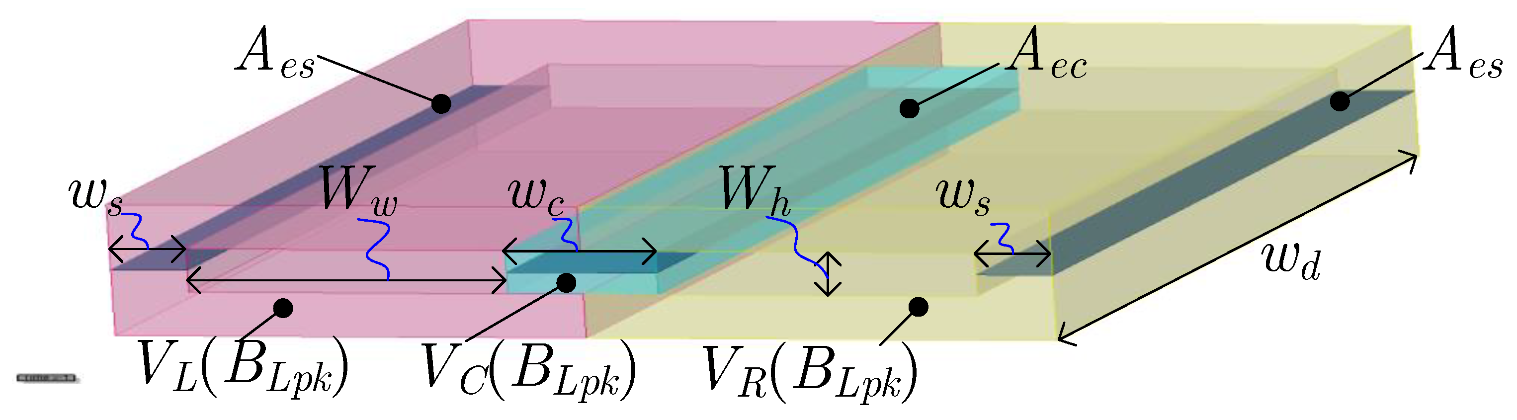
4.1. Derivation of the Core Loss (P_c)

With i_r1, i_r2 and i_m applied to L_r1, L_r2 and L_m, the flux density of V_L, V_R and V_C, B_Lpk, B_Rpk and B_Cpk, can be calculated by:

$$\begin{gathered} B_{Lpk}=\frac{L_{r1}}{N_{r1}{A}_{es}}{I}_{r1pk}+\frac{L_{r2}}{N_{r2}{A}_{es}}{I}_{r2pk}+\frac{L_m}{2N_p{A}_{ec}}{I}_{mpk} \\ {B}_{Rpk}=\frac{L_{r1}}{N_{r1}{A}_{es}}{I}_{r1pk}+\frac{L_{r2}}{N_{r2}{A}_{es}}{I}_{r2pk}-\frac{L_m}{2N_p{A}_{ec}}{I}_{mpk} \\ {B}_{Cpk}=\frac{L_m}{N_p{A}_{ec}}{I}_{mpk} \end{gathered}$$

(13)

where I_r1pk, I_r2pk and I_mpk are the peak values of i_r1, i_r2 and i_m, respectively. V_L, V_C and V_R are illustrated by Figure 7. A_es and A_ec are the cross-sectional area of the side leg and central leg, which are also shown in Figure 7.

Based on the Steinmetz’s formula, combining Equation (13), the total core loss of the magnetic core can be calculated by:

$$P_c=k_c{f}_s^a{B}_{Lpk}^b{V}_L+k_c{f}_s^a{B}_{Rpk}^b{V}_R+k_c{f}_s^a{B}_{Cpk}^b{V}_C$$

(14)

where k_c, α and β are the parameters of the magnetic core, which can be found from the datasheet.

The equation of total core loss P_c will be used for the further optimal design.

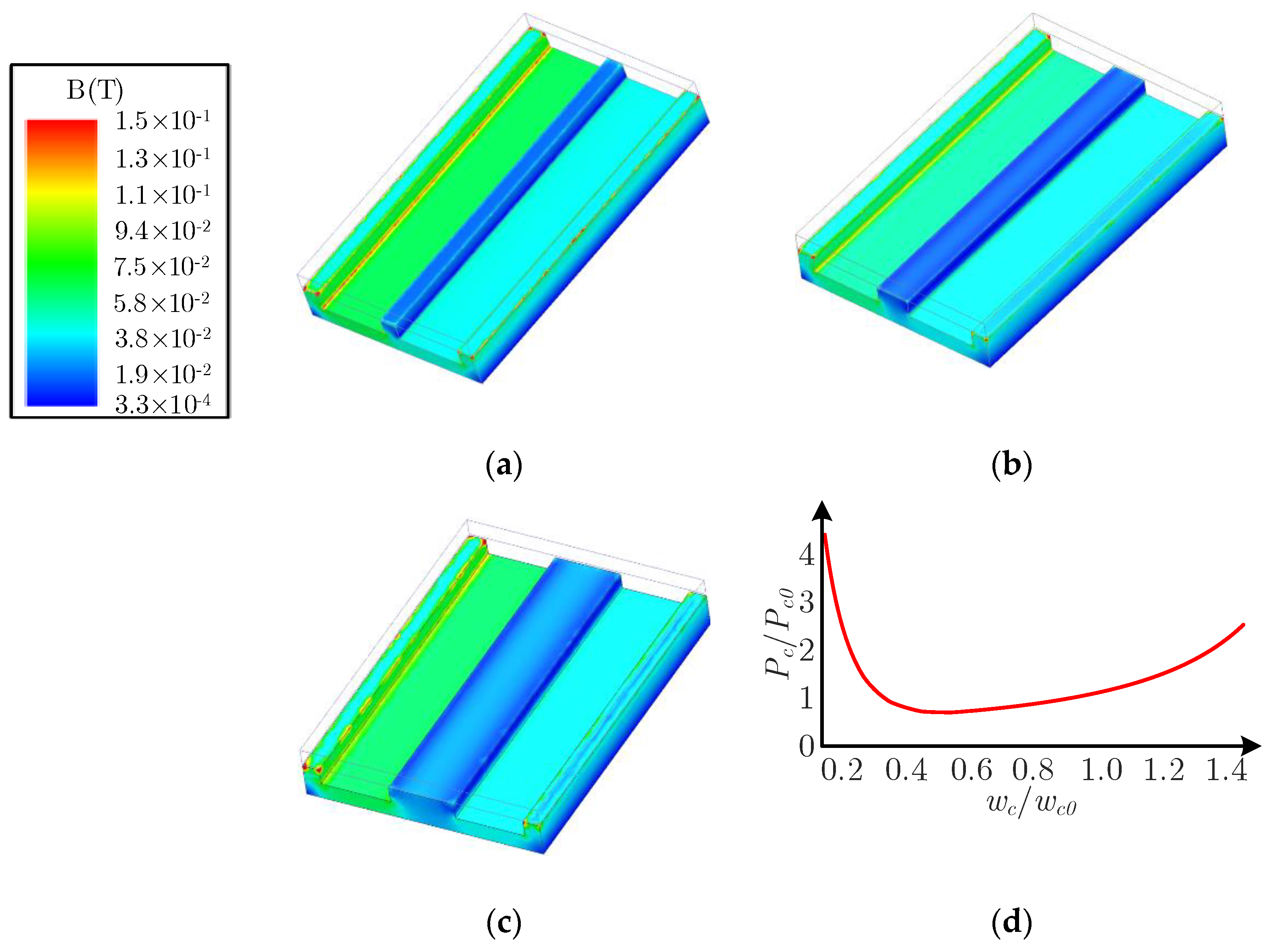
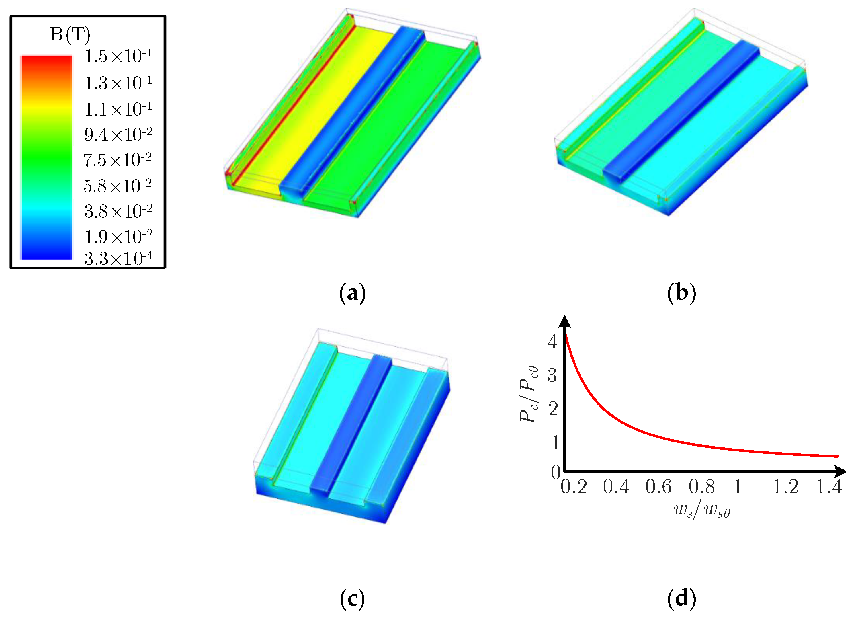
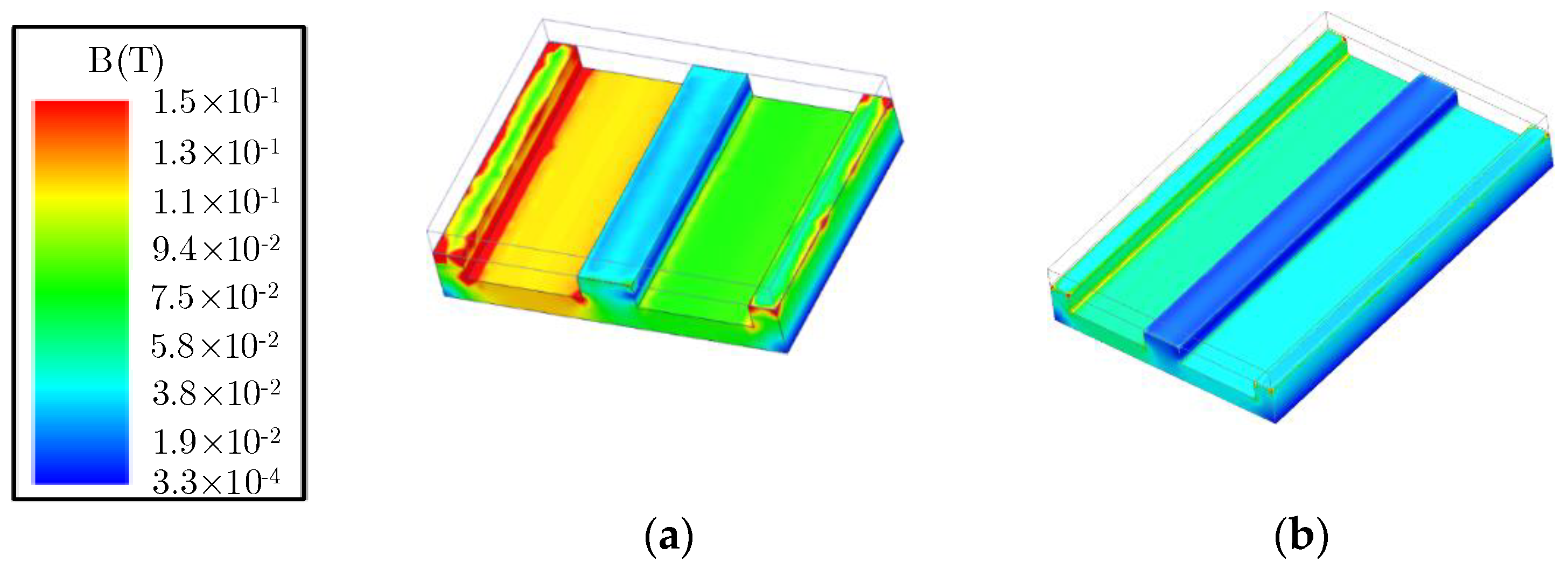
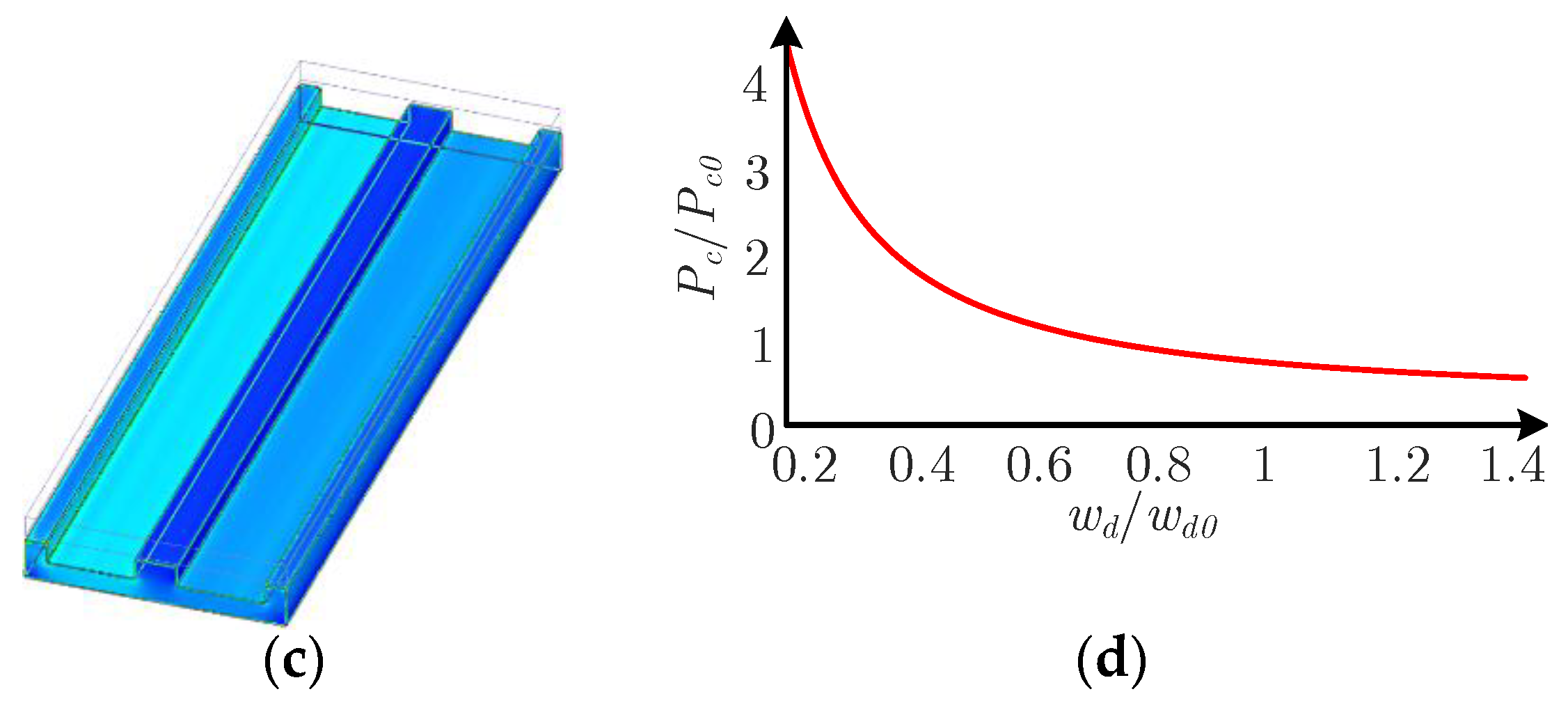
4.2. Effects of w_s, w_c, and w_d on the Total Core Loss P_c

The effects of w_s, w_c, and w_d on P_c are studied in this part. The selected magnetic core is ELP 64/10/50 with N87, from TDK. In order to increase the power rating, two magnetic cores are used in parallel to increase the cross-sectional area. The sizes of the magnetic core are shown in

Table 2. The Sizes of the magnetic core.

Symbol	Values	Symbol	Values
wc	10.4 mm	ww	21.7 mm
ws	5.2 mm	wb	10.4 mm
wd	101.6 mm	Aes	519 mm2
Aec	1038 mm2	-	-

, which will be used as the base values in the following comparison.

In order to make a fair comparison, all the cases in the following share the same winding configuration, which is the same with that in Figure 6b.

The current excitations are from the circuit simulation of a CLLC resonant converter. The parameters of the CLLC resonant converter as well as the current excitations are shown in

Table 3. The Parameters of the CLLC resonant converter and the current excitations.

Symbol	Values	Symbol	Values
Vin	200 V	Vo	200 V
fs	100 kHz	Po	500 W
Lrp	30 µH	Lrps	30 µH
Lm	550 µH	Ir1pk	4.05 A
Ir2pk	4.0 A	Impk	0.54 A

.

(a) Effect of w_c on Core Loss

In the first case, the width of the center leg, w_c, is changed from 20 to 140% of the base value (10.4 mm), while other parameters are kept the same with the base values. Simulations are carried out in Ansys Maxwell and the distributions of the magnetic flux density are shown in Figure 8.

It can be seen from Figure 8 that although w_c is reduced as shown in Figure 8a or increased as shown in Figure 8c the magnetic flux density is still low, which may be further optimized. This is because in the proposed integrated magnetic structure, the flux mainly concentrates on the side legs. The variation of P_c with different w_c is calculated, which is shown in Figure 8d. All the parameters in Figure 8d are in per-unit-value. The original w_c, w_c0 (10.4 mm) and the corresponding core loss, P_c0 (5.8 W) are used as the based value.

It can be seen from Figure 8d considering the volume and the core loss, the central leg of the magnetic core can be further optimized.

(b) Effect of w_s on Core Loss

In the second case, the width of the side legs, w_s, is changed from 20 to 140% of the base value (5.2 mm), while other parameters are kept the same with the base values. Simulations are carried out in Ansys Maxwell and the distributions of the magnetic flux density are shown in Figure 9.

It can be seen from Figure 9 that compared with Figure 9b as w_s is reduced in Figure 9a the magnetic flux density in the side leg will increase. In contrast, compared with Figure 9b, in Figure 9c, as w_s is increased, the magnetic flux density in the side leg will decrease. The variation of P_c with different w_s is calculated, which is shown in Figure 9d. All the parameters in Figure 9 are in per-unit-value. The original w_s, w_s0 (5.2 mm) and the corresponding core loss, P_c0 (5.8 W) are used as the base values.

It can be seen from Figure 9d that with larger w_s, the magnetic flux density in the side leg will decrease and the core loss will decrease. It is because that the flux in the side legs is enhanced due to coupling between L_r1 and L_r2. As a result, in order to achieve better performance for a specific application, the side legs need further optimization.

(c) Effect of w_d on Core Loss

In the third case, the depth of the magnetic core, w_d, is changed from 20 to 140% of the base value (101.6 mm), while other parameters are kept the same with the base values. Simulations are carried out in Ansys Maxwell and the distributions of the magnetic flux density are shown in Figure 10.

It can be seen from Figure 10 that compared with Figure 10b, as w_d is reduced in Figure 10a, the magnetic flux density in the side leg will increase. In contrast, compared with Figure 10b, as w_d is increased in Figure 10c, the magnetic flux density in the center leg will decrease. The variation of P_c with different w_d is calculated, which is shown in Figure 10.

It can be seen from Figure 10 that with the increase of w_d, the core loss will decrease. It is because that the flux in the side legs is enhanced due to coupling between L_r1 and L_r2. As a result, in order to achieve better performance for a specific application, the depth of the core need further optimization, which is similar to the effect of w_s.

Based on the above analysis, it can be concluded that the core loss of the magnetic core is affected by w_s, w_c, and w_d. In order to achieve low core loss, w_s, w_c, and w_d need further optimization. However, it is important to point out that the core loss and the volume of the magnetic core always contradict each other: lower core loss means larger volume of the magnetic core while lower volume of the magnetic core means higher core loss. Considering both core loss and the volume of the core, in the following part, the tradeoff design of the proposed integrated magnetic structure based on Pareto Frontier will be investigated.

4.3. Tradeoff Design of the Proposed Integrated Magnetic Structure Based on Pareto Optimization Procedure

The Pareto optimization [18,19] is utilized to identify the best performing proposed integrated magnetic structure for a CLLC resonant converter. The specifications of the converter and the magnetic material are required for the calculations of the volume and power loss of the magnetic core. Each parameter within the limits of the design space is swept individually, resulting in dataset where each point represents an integrated magnetic design and its corresponding performance, including the volume and power loss of the core. By analyzing the volume and core loss, the Pareto frontier can be revealed, which represents the lowest achievable magnetic core loss for a given volume.

(a)

Flowchart of Pareto optimization procedure for the proposed integrated magnetic structure

The flowchart of the proposed integrated magnetic structure Pareto optimization procedure is shown in Figure 11.

The details of each step are as follows:

Step 1: Initialization of Pareto optimization procedure

The operation conditions of the CLLC resonant converter, O = {I_r1pk, I_r2pk, I_mpk}, which are derived from the circuit simulations, are set. The design space, W_d = {40.64 mm ≤ w_d ≤ 160.4 mm}, W_c = {4.08 mm ≤ w_c ≤ 15.3 mm}, W_s = {2.08 mm ≤ w_s ≤ 7.80 mm}, which are used to limit the dimensions of the magnetic core, are defined.

The population, X_j = {x₁, x₂, …, x_i, …, x_N}, where x_i = {w_di, w_ci, w_si}, are initialized.

Step 2: Calculations of the dominated number of each individual (n_p) and crowding distance (C_d)

In this step, at first, the multi-objective values, the volume of the magnetic core, V_c, and the core loss, P_c, are calculated. n_p and C_d of each individual are calculated with V_c and P_c based on non-dominated sorting.

Step 3: Evolution of the population

The population, X_j = {x₁, x₂, …, x_i, …, x_N}, evolves, including selection, crossover and mutation. After evolvement, the new population, X_newj = {x_new1, x_new2, x_newi, …, x_newN}, is generated.

After generation of X_newj, X_j and X_newj are combined together to form a population X_2Nj, which includes 2N individuals.

Step 4: Recycling of Step 2 and Step 3

In this step, if the maximum iteration number is reached, the recycling process stops. Otherwise, N individuals will be chosen for X_j as the next generation and the new recycling process of Step 2 and Step 3 will begin.

Step 5: Generate the Pareto frontier

After the maximum iteration number is reached, the recycling process stops, and the Pareto frontier will be generated.

(b)

Application of Pareto optimization procedure for the proposed integrated magnetic structure

In this part, the Pareto optimization is used for the design of the proposed integrated magnetic structure in a CLLC resonant converter. The specifications of the CLLC resonant converter are shown in Table 3. The magnetic material is N87, from TDK. With the flowchart shown in Figure 11, the generated Pareto Frontier is shown in Figure 12. The conventional design, where the leakage inductances are used as the resonant inductances is also shown in Figure 12 (Point B) for comparison.

It can be seen from Figure 12 that with the increase of the magnetic core volume, the core loss will decrease. However, the volume of the magnetic core cannot be increased unboundedly. In a specific application, there is trade-off design between the volume and the power loss.

In addition, under the same volume condition, the core loss on the Pareto frontier is lower than the conventional design, which means that with optimal design, the proposed integrated magnetic structure can achieve not only high-power density but also low power loss. The optimal dimensions of the magnetic core are w_s = 3.82 mm, w_c = 6.64 mm, and w_d = 152.39 mm.

The conventional design and the optimal design based on Pareto Frontier will be validate by simulations in the following section.

5. Simulation and Experimental Validations of the Proposed Integrated Magnetic Structure and the Pareto Optimization Procedure

In this section, the proposed integrated magnetic structure and the Pareto optimization procedure are validated by the hybrid electromagnetic simulations and experiments. Three cases are considered in this section:

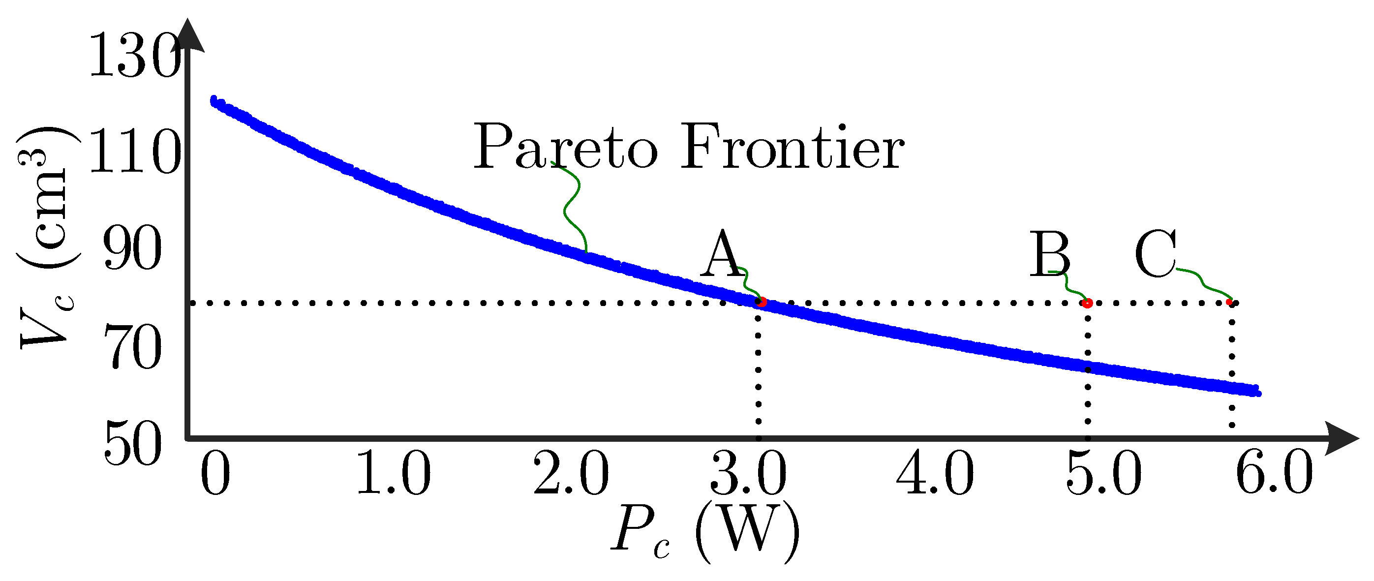
• Conventional design, Point B, as shown in Figure 12, where the leakage inductances are used as the resonant inductances.
• Unoptimized design of the proposed integrated magnetic structure, Point C, as shown in Figure 12.
• Optimal design of the proposed integrated magnetic structure based on Pareto frontier, Point A, as shown in Figure 12.

5.1. Simulation Validations

The parameters of the CLLC resonant converter are shown in Table 3. The simulated magnetic flux density of the conventional design, unoptimized design of the proposed integrated magnetic structure, and optimized design of the proposed integrated magnetic structure are shown in Figure 13a–c, respectively.

Based on the distributions of the magnetic flux density, the core loss of each design is calculated, which is shown in Figure 13d.

It can be seen from Figure 13d that the core loss of the unoptimized design of the proposed integrated magnetic structure is higher than the conventional design. This is because the current of L_rp and L_rs flowing through the side legs of the magnetic core causes extra core loss. However, with the Pareto optimization procedure, the core loss of the optimized design of the propose integrated magnetic structure is reduced, which is lower than the conventional design.

As a result, it can be concluded that with the Pareto optimization procedure, the proposed integrated magnetic structure can enjoy higher power density and lower core loss compared with the conventional design. In the following part, the conventional design, unoptimized proposed integrated magnetic structure and the Pareto frontier based optimized proposed integrated magnetic structure will be further validated by the experiments.

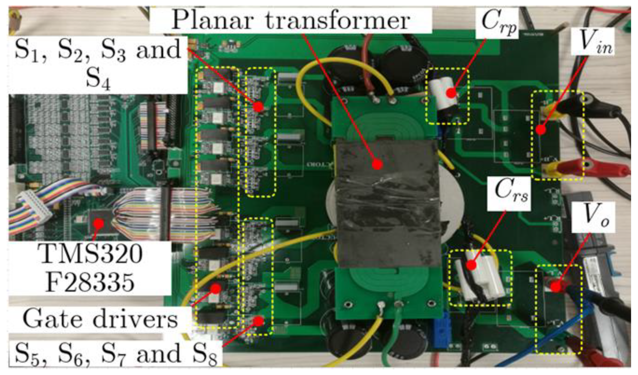
5.2. Experimental Validation of the Proposed Integrated Magnetic Structure and Its Corresponding Pareto Optimization Procedure

Three planar transformers are designed for validations: conventional planar transformer structure, as shown in Figure 14a; unoptimized proposed integrated magnetic structure, as shown in Figure 14b; optimized proposed integrated magnetic structure, as shown in Figure 14c.

L_r1, L_r2, L_rp, L_rs, and L_m are set by changing the air gaps in the central leg (d_c) and the side legs (d_s) and are measured by the impedance analyzer. The measured results of the inductances in each structure are shown in

Table 4. Measured results.

Parameters	Conventional	Unoptimized	Optimized
Lr1 (µH)	29.8	14.82	14.86
Lr2 (µH)	29.8	14.82	14.86
Lrp (µH)	29.8	29.6	29.7
Lrs (µH)	29.8	29.6	29.7
Lm (µH)	542	545	543

.

It can be seen from Table 4 that by adjusting d_c and d_s, all the three planar transformers share the same resonant inductances, L_rp and L_rs, and the same magnetizing inductance L_m. In the following part, all the three planar transformers will be tested in the CLLC resonant converter to further validate the proposed integrated magnetic structure and its corresponding Pareto optimization procedure.

The planar transformers shown in Figure 14 are tested in the CLLC resonant converter. The main switches and the rectifiers are C2M0080120D (Silicon Carbide), from CREE and the controller is TMS320F28335. The parameters of the CLLC resonant converter are the same with the parameters in Table 3. The CLLC resonant converter with the planar transformer is shown in Figure 15, where all the three transformers shown in Figure 14 will be tested.

(a)

Working principle validations of the proposed integrated magnetic structure

In order to validate the working principles of the proposed integrated magnetic structure, the transformers in Figure 14 are tested in the CLLC resonant converter. The experimental waveforms of the output of the full bridge in the primary side, v_AB(t), the output of the full bridge in the secondary side, v_CD(t), and the current in the primary side, i_p(t) in the three designs are shown in Figure 16, where Figure 16a shows the experimental waveforms with the conventional planar transformer; Figure 16b shows the experimental waveforms with the unoptimized proposed integrated magnetic structure; and Figure 16c shows the experimental waveforms with the optimized proposed integrated magnetic structure.

It can be seen from Figure 16a that the switching frequency of the CLLC resonant converter with the conventional planar transformer is 100 kHz, which is in accordance with the design. In addition, both the initial magnetic integration, as shown in Figure 16b, and the optimized magnetic integration, as shown in Figure 16c, share the same experimental waveforms as Figure 16a, which means the design of the resonant inductances, L_rp and L_rs, and the magnetizing inductance, L_m, has been achieved by the proposed magnetic integration.

However, it is important to point out that it is necessary to further investigate the power efficiency of the converter with the proposed integrated magnetic structure.

(b)

The power efficiency of the CLLC resonant converter with the proposed magnetic integration

It has been proven in the previous part that the proposed magnetic integration can be used for the CLLC resonant converter. In this part, the power efficiency of the CLLC resonant converter with the proposed magnetic integration will be further investigated.

The power efficiency of the CLLC resonant converter with three different transformers in Figure 14 under different output power is tested and the experimental results are shown in Figure 16d.

It can be seen from Figure 16d that compared with the conventional planar transformer, where the leakage inductances are used as the resonant inductances, the efficiency of the unoptimized proposed integrated magnetic structure is lower. This is because that the magnetic flux density increases due to the magnetic integration. As a result, both the copper loss and the core loss will increase.

In addition, it can be seen from Figure 16d that the efficiency of the CLLC resonant converter with the optimized integrated magnetic structure is higher than that with the conventional transformer. Thanks to the Pareto optimization procedure, the distributions of the magnetic flux density are optimized, and the power loss of the magnetic core is reduced.

It is worth pointing out that the selection of the design from the Pareto frontier, Point A, as shown in Figure 12, is based on the same magnetic core volume, which is used as an example. The selection of the design from the Pareto frontier is the trade-off between the volume and the power loss, which is dependent on the specific application. However, it has been proven that the proposed Pareto optimization procedure based integrated magnetic structure can achieve higher efficiency than the conventional planar transformer under the same volume.

6. Conclusions

An integrated magnetic structure for the CLLC resonant converter has been proposed in this paper. Two resonant inductances and a transformer are integrated into a magnetic core. Compared with the conventional planar transformer, where the leakage inductances are used as the resonant inductances, the advantages of the proposed integrated magnetic structure can be summarized as follows:

Firstly, the extra height of the magnetic core, which is used to generate the desired leakage inductances in the conventional planar transformer is not required anymore. As a result, the volume of the core will be reduced.

Secondly, as the leakage flux stored between primary winding and secondary winding is reduced, the copper loss caused by the proximity effect will be improved.

Thirdly, with the proposed integrated magnetic structure, the range of the leakage inductances is extended, which can be easily changed by the number of turns in the resonant inductances.

Finally, the multi-objective optimization method, Pareto optimization procedure, is utilized for the optimal design of the proposed integrated magnetic structure and high efficiency can be achieved.

The advantages of the proposed integrated magnetic structure have been validated by the simulations and experiments.

References

1. Zhang, Z.; Ouyang, Z.; Thomsen, O.C.; Andersen, M.A.E. Analysis and Design of a Bidirectional Isolated DC–DC Converter for Fuel Cells and Supercapacitors Hybrid System. IEEE Trans. Power Electron. 2012, 27, 848–859. [Google Scholar] [CrossRef] [Green Version]
2. Ouyang, Z.; Zhang, Z.; Thomsen, O.C.; Andersen, M.A.E. Planar-Integrated Magnetics (PIM) Module in Hybrid Bidirectional DC–DC Converter for Fuel Cell Application. IEEE Trans. Power Electron. 2011, 26, 3254–3264. [Google Scholar] [CrossRef] [Green Version]
3. Huang, L.; Zhang, Z.; Andersen, M.A.E. Analytical Switching Cycle Modeling of Bidirectional High-Voltage Flyback Converter for Capacitive Load Considering Core Loss Effect. IEEE Trans. Power Electron. 2016, 31, 470–487. [Google Scholar] [CrossRef] [Green Version]
4. Thummala, P.; Schneider, H.; Zhang, Z.; Andersen, M.A.E. Investigation of Transformer Winding Architectures for High-Voltage (2.5 kV) Capacitor Charging and Discharging Applications. IEEE Trans. Power Electron. 2016, 31, 5786–5796. [Google Scholar] [CrossRef]
5. Zhao, B.; Song, Q.; Liu, W.; Sun, Y. Overview of Dual-Active-Bridge Isolated Bidirectional DC–DC Converter for High-Frequency-Link Power-Conversion System. IEEE Trans. Power Electron. 2014, 29, 4091–4106. [Google Scholar] [CrossRef]
6. Jung, J.H.; Kim, H.S.; Ryu, M.H.; Baek, J.W. Design Methodology of Bidirectional CLLC Resonant Converter for High-Frequency Isolation of DC Distribution Systems. IEEE Trans. Power Electron. 2013, 28, 1741–1755. [Google Scholar] [CrossRef]
7. Huang, J.; Zhang, X.; Shuai, Z.; Zhang, X.; Wang, P.; Koh, L.H.; Xiao, J.; Tong, X. Robust Circuit Parameters Design for the CLLC-Type DC Transformer in the Hybrid AC/DC Microgrid. IEEE Trans. Ind. Electron. 2018, 66, 1906–1918. [Google Scholar] [CrossRef]
8. Ryu, M.H.; Kim, H.S.; Baek, J.W.; Kim, H.G.; Jung, J.H. Effective Test Bed of 380-V DC Distribution System Using Isolated Power Converters. IEEE Trans. Ind. Electron. 2015, 62, 4525–4536. [Google Scholar] [CrossRef]
9. Gao, Y.; Sun, K.; Lin, X.; Guo, Z. A Phase-Shift-Based Synchronous Rectification Scheme for Bi-Directional High-Step-Down CLLC Resonant Converters. In Proceedings of the 2018 IEEE Applied Power Electronics Conference and Exposition (APEC), San Antonio, TX, USA, 4–8 March 2018; pp. 1571–1576. [Google Scholar]
10. Liu, G.; Li, D.; Zhang, J.Q.; Hu, B.; Jia, M.L. Bidirectional CLLC Resonant DC-DC Converter with Integrated Magnetic for OBCM Application. In Proceedings of the 2015 IEEE International Conference on Industrial Technology (ICIT), Seville, Spain, 17–19 March 2015; pp. 946–951. [Google Scholar]
11. Li, B.; Li, Q.; Lee, F.C. A WBG based three phase 12.5 kW 500 kHz CLLC resonant converter with integrated PCB winding transformer. In Proceedings of the 2018 IEEE Applied Power Electronics Conference and Exposition (APEC), San Antonio, TX, USA, 4–8 March 2018; pp. 469–475. [Google Scholar]
12. Zou, S.; Lu, J.; Mallik, A.; Khaligh, A. Bi-Directional CLLC Converter with Synchronous Rectification for Plug-In Electric Vehicles. IEEE Trans. Ind. Appl. 2018, 54, 998–1005. [Google Scholar] [CrossRef]
13. Zahid, Z.U.; Dalala, Z.M.; Chen, R.; Chen, B.; Lai, J.S. Design of Bidirectional DC–DC Resonant Converter for Vehicle-to-Grid (V2G) Applications. IEEE Trans. Transp. Electrif. 2015, 1, 232–244. [Google Scholar] [CrossRef]
14. He, P.; Khaligh, A. Design of 1 kW Bidirectional Half-Bridge CLLC Converter for Electric Vehicle Charging Systems. In Proceedings of the 2016 IEEE International Conference on Power Electronics, Drives and Energy Systems (PEDES), Trivandrum, Kerala, India, 14–17 December 2016; pp. 1–6. [Google Scholar]
15. Ouyang, Z.; Zhang, J.; Hurley, W.G. Calculation of Leakage Inductance for High-Frequency Transformers. IEEE Trans. Power Electron. 2015, 30, 5769–5775. [Google Scholar] [CrossRef]
16. Zhang, J.; Ouyang, Z.; Duffy, M.C.; Andersen, M.A.E.; Hurley, W.G. Leakage Inductance Calculation for Planar Transformers with a Magnetic Shunt. IEEE Trans. Ind. Appl. 2014, 50, 4107–4112. [Google Scholar] [CrossRef] [Green Version]
17. Zhao, B.; Ouyang, Z.; Duffy, M.; Andersen, M.A.E.; Hurley, W.G. An Improved Partially Interleaved Transformer Structure for High-voltage High-frequency Multiple-output Applications. IEEE Trans. Ind. Electron. 2018, 66, 2691–2702. [Google Scholar] [CrossRef] [Green Version]
18. Deb, K.; Pratap, A.; Agarwal, S.; Meyarivan, T. A fast and elitist multiobjective genetic algorithm: NSGA-II. IEEE Trans. Evol. Comput. 2002, 6, 182–197. [Google Scholar] [CrossRef] [Green Version]
19. Andersen, T.M.; Krismer, F.; Kolar, J.W.; Toifl, T.; Menolfi, C.; Kull, L.; Morf, T.; Kossel, M.; Brändli, M.; Francese, P.A. Modeling and Pareto Optimization of On-Chip Switched Capacitor Converters. IEEE Trans. Power Electron. 2017, 32, 363–377. [Google Scholar] [CrossRef]
Figure 1. The CLLC resonant converter.
Energies 14 01756 g001
Figure 2. Magnetic design for a CLLC resonant converter: (a) Detached magnetic cores; (b) conventional integrated magnetic structure; (c) proposed integrated magnetic structure.
Energies 14 01756 g002
Figure 3. General winding configuration and magneto-motive force (MMF) distribution.
Energies 14 01756 g003
Figure 4. Magnetic flux analysis of the proposed integrated magnetics.
Energies 14 01756 g004
Figure 5. Equivalent magnetic circuit with the excitation of: (a) ir1; (b) ir2; (c) im.
Energies 14 01756 g005
Figure 6. 2D structure of the magnetics and their simulation results with: (a) Conventional structure; (b) Proposed integrated magnetic structure.
Energies 14 01756 g006
Figure 7. 3D model of a magnetic core.
Energies 14 01756 g007
Figure 8. Distribution of magnetic flux density with different wc: (a) wc = 5.2 mm; (b) wc = 10.4 mm; (c) wc = 20.8 mm; (d) core loss with wc.
Energies 14 01756 g008
Figure 9. Distribution of magnetic flux density with different ws: (a) ws = 52.6 mm; (b) ws =5.2 mm; (c) ws = 10.4 mm; (d) core loss with ws.
Energies 14 01756 g009
Figure 10. Distribution of magnetic flux density with different wd: (a) wd = 50.8 mm; (b) wd = 101.6 mm; (c) wd = 203.2 mm; (d) core loss with wd.
Energies 14 01756 g010aEnergies 14 01756 g010b
Figure 11. Flowchart of the Pareto optimization procedure of the proposed integrated magnetic structure.
Energies 14 01756 g011
Figure 12. Pareto frontier of the proposed integrated magnetic structure: A: selected optimal design of the proposed integrated magnetic structure; B: conventional design; C: unoptimized design of the proposed integrated magnetic structure.
Energies 14 01756 g012
Figure 13. Simulation results: (a) conventional design; (b) unoptimized design of the proposed integrated magnetic structure; (c) optimized design of the proposed integrated magnetic structure; (d) power loss comparison.
Energies 14 01756 g013
Figure 14. The planar transformers of CLLC resonant converter for validations: (a) conventional planar transformer; (b) unoptimized proposed integrated magnetic structure; (c) optimized proposed integrated magnetic structure.
Energies 14 01756 g014
Figure 15. The CLLC resonant converter for the validation.
Energies 14 01756 g015
Figure 16. Experimental waveforms: (a) conventional planar transformer; (b) unoptimized proposed integrated magnetic structure; (c) optimized proposed integrated magnetic structure; (d) efficiency comparison.
Energies 14 01756 g016