Analysis of Harmful Exhaust Gas Concentrations in Cloud behind a Vehicle with a Spark Ignition Engine

Abstract

The article presents issues related to the assessment of concentrations of harmful substances in the exhaust gas cloud behind the vehicle. In the theoretical part, considerations about the harmfulness of exhaust gases and methods of detection of chemical compounds were made, and the issues of von Karman vortices and the Lambert-Beer law were referred to. The test object was a vehicle equipped with an SI engine meeting the Euro 3 standard. The drive unit had a capacity of 2.8 dm³, a rated power reaching 142 kW at 5500 rpm and a maximum torque of 280 Nm at 3500 rpm. The measurements of the dilution of the exhaust gas cloud behind the vehicle were made in stationary conditions (laboratory) and during actual operation in the Poznań agglomeration. In the research, technically advanced equipment from the PEMS group was used. In the analysis of the obtained results, detailed considerations were made regarding the influence of the location of the measuring probe in relation to the exhaust system. As can be seen from the obtained dependencies, the vehicle motion is favorable for the assessment of concentrations behind a moving object, because the ecological indicators at successive distances behind the exhaust system achieve better parameters in most points than in a stationary test.

1. Introduction

Air pollution is one of the leading causes of global health problems. Today, nine out of ten people breathe polluted air, which causes premature deaths of more than 4 million people each year. The International Agency for Research on Cancer in 2013 [1] concluded that toxic compounds in the exhaust gases in the air are carcinogenic, and that particulate matter causes a greater incidence of cancer. One of the causes of environmental degradation is the presence of increasing numbers of cars on the roads. In particular, old and worn-out cars constitute a significant portion of vehicles and machines equipped with internal combustion engines. Vehicle exhaust gases are much more harmful to humans than industrial exhaust gases because the exhaust gases spread in high concentrations at low altitudes in the immediate vicinity of people [1]. Environmental issues in the automotive industry are currently significant challenges. In the transport sector, the vast majority of propulsion systems are still internal combustion engines. Within their development, many advanced works related to the improvement of the combustion process are carried out, including improvement of the fuel injection process, including DI [2,3] and optimization of EGR parameters [4]. The aspect of fuels is also important, which has been broadly presented in the literature [5,6,7].

Papers such as [8,9,10,11] present considerations concerning the measurements of pollutants in the exhaust gas cloud behind the vehicle using remote sensing technologies. Remote sensing technology allows one to measure vehicle emissions without disrupting traffic. It is possible to measure a large number of vehicles in a short time, at low unit costs, where a one-second shutter of exhaust from the vehicle is recorded. This registration method is commonly used in at least 27 countries. China was the first in the world in 2017 to introduce legal regulations on exhaust emissions measurements using remote sensing at the national level. Remote sensing systems mainly measure NO, CO, HC, CO₂ and PM (indirectly from the exhaust cloud opacity). However, the emission limits defined only cover the emission of nitrogen oxides and particulate matter. The measurement of NO is only a check for high-emission vehicles. Paper [8] explains the current lack of accuracy in estimating the NO concentration in the exhaust system of vehicles equipped with a compression-ignition engine. Remote sensing measures the pollutant concentration ratio in the exhaust gas cloud as there is no way yet to accurately estimate the NO concentration in the exhaust gas of vehicles powered by a diesel engine. The paper also describes methods of alternative measurement of nitrogen oxides. The report [9] presents the existing limitations in the applications of remote sensing. The barriers were divided into categories: equipment and measurements, data availability and analysis and logistics and cost. In the articles [10,11] the results of tests carried out with the use of remote sensing have been presented. The Paris emission test [10] was carried out with an EDAR (Emissions Detection and Reporting) instrument, using a laser light source passing across the width of the road and through the exhaust cloud of the measured vehicle. The key conclusions obtained in the article refer to the emission of nitrogen oxides. The results showed that NO_x emissions from Euro 6 diesel cars in Paris are 4.8 times greater than from Euro 6 gasoline cars for the specified distances and 6 times greater than results obtained in laboratory conditions. In addition, it was shown that diesel cars (both Euro 5 and Euro 6) were responsible for 63% of total NO_x emissions from passenger cars in Paris during the road test. The authors of the paper [11] arrived at similar conclusions. The article also compares the obtained results with the measurements from the CONO_x project. This project aims to collect remote sensing exhaust emission results from different countries and to create a European remote sensing database. Such a comparison was also made in the article on the emissions test in Zurich [11]. The analyses of mean NO_x emission values that have been carried out for this publication confirm the conclusions of previous studies: actual emissions from gasoline vehicles are significantly lower than those from vehicles with a diesel engine. Exhaust emission from diesel engines remained practically unchanged between Euro 4 and Euro 5 and all vehicle groups with diesel engines from Euro 3 to Euro 6 exceed the limits of the exhaust emission norms.

This article presents the analysis results of the harmful substances concentration in the exhaust gas cloud behind a vehicle, both in stationary tests and in motion, for vehicles equipped with a spark ignition engine. For this purpose, a PEMS (Portable Emissions Measurement System) type apparatus was used because it enables the recording of exhaust emissions from a vehicle while traveling on a long route [12,13,14,15,16,17,18]. Moreover, it is characterized by the direct measurement of road emissions of vehicles in a wide spectrum of engine and drive systems operating points. The apparatus used was equipped, among others, with an NDIR (Non-Dispersive Infra-Red) analyzer, using a measurement method which uses absorption spectroscopy based on the Beer-Lambert law, which describes quantitatively the weakening (resulting from absorption) of the light beam passing through the substance layer [19]. The tests were carried out at four measuring points at different distances and at different heights from the exhaust gas system.

This equipment was chosen because of the ability to precisely measure harmful exhaust gas compounds. In the future, the performed tests will constitute the basis for verifying the functioning of the emission gate operating on the basis of remote sensing. The emission gate will be a tool for the remote measurement of all limited gaseous compounds (CO, NO, NO₂, HC), carbon dioxide, particulate matter in terms of concentration, number and dimensional distribution, as well as exhaust smoke for a wide range of vehicles of various categories in motion. The device will enable a quick assessment of emissions from passing vehicles and, consequently, their immediate elimination from traffic if the accepted standards are exceeded. The proposed solution will be able to use the open-path or extractive method depending on the priority guidelines for the conducted research. The exhaust gases will be collected by the device using a special design of probes made in such a way that air samples will be collected from the space directly adjacent to the exhaust gas exhaust system of the tested vehicles, while passing through the measuring gate.

2. Optical Measurement Method

The optical measurement method is based on the rules of optics and consists of comparing the intensity of the light beam passing through the tested medium with the intensity of the light beam that was sent through the reference gas (Figure 1). The exhaust emissions concentration is measured as the decrease in gas transparency caused by the effects of absorption and dispersion. The accuracy of the measurement depends on the optical properties, chemical composition and particle size. An example of such an optical measurement method is the NDIR method in which infrared light is used and the NDUV where ultraviolet light is used.

In research with the use of optical measurement methods, the laws related to absorbance (the ability to absorb radiation) are used. Beer’s law states that the amount of light absorbance of a solution is directly proportional to the concentration of the light absorbing substance (Figure 2). The Lambert-Beer (Beer-Lambert-Bouguer) law describes the absorption of electromagnetic radiation when passing through a partially absorbing and scattering medium [21].

The Lambert-Beer law states that the degree of attenuation (taking into account absorption and scattering) of light is proportional to the thickness of the layer and its optical properties. For solutions, the molar concentration of the absorbing substance should be taken into account. The law is true for both monochromatic and collimated light beams. It is also used in the situation of narrow band ranges, especially if the spectral dependence of attenuation is not strong in this band. The recorded intensity I₀ is also the intensity of monochromatic and collimated light. The final value of the radiation intensity I₁ is lower than I₀ by the value of the radiation absorption intensity. This law can be expressed mathematically in several different ways [21].

$$\frac{I_1}{I_0}=e^{-\alpha lc}$$

(1)

$$A= \mathsf{\epsilon }lc$$

(2)

$$A=lo{g}_{10}\frac{I_0}{I_1}$$

(3)

where:

• A—absorbance,
• I₀—the intensity of the light going in the sample,
• I₁—the intensity of light after passing through the sample,
• ε—molar extinction coefficient,
• l—the path light travels in the sample,
• c—the molar concentration of the absorbent in the solution,
• α—molar absorption coefficient correctly called molar absorbance.

A vehicle in motion is subject to forces associated with the drive train system, tire friction and aerodynamic drag. Movement causes air molecules to pile up as they approach the vehicle’s face. As a result, there is a local increase in pressure. At the same time, the pressure in the streams flowing around the car body is close to the atmospheric pressure. This causes the air to move towards the area of lower pressure, trying to achieve equilibrium. As a result of the continuous movement of the vehicle and the accumulation of particles, air flows are formed around the vehicle body, while a sphere with properties similar to a vacuum is created directly behind it. This is directly related to the speed with which the vehicle is moving. When driving at a high speed, air particles are not able to fill the space that is directly behind the vehicle quickly enough. Rapid pressure change and the inertia of air molecules affect the occurrence of the phenomenon of flow separation known from aviation. It occurs when the boundary layer moves so far away from the pressure gradient that its velocity is almost zero compared to that of the moving vehicle. This separation makes the flow turbulent and its path chaotic [22]. Figure 3 shows an example of simulation performed in ANSYS showing a method for forming a turbulent flow zone for the moving vehicle.

In the case of a flow around a vehicle body that has non-aerodynamic shapes, the flow separation occurs at its edge. This phenomenon does not depend on the Reynolds number, which allows one to estimate the ratio of inertia forces to viscous forces occurring during the movement of the tested medium. It determines the type of particle movement. Laminar (stratified) motion is characterized by a parallel location of the planes of motion (Re ≤ 2300), while in chaotic (turbulent) motion the directions of particle motions intersect and cause collisions (Re > 50,000). The Reynolds number is expressed as a relation [22,23].

$$Re·\frac{\rho ·u·l}{\mu } or Re·\frac{u·l}{\nu }$$

(4)

where:

• $\rho$—the tested medium density [kg/m³],
• u—characteristic velocity of the tested medium (average velocity relating to the total flow) [m/s],
• l—characteristic dimension of the problem (distance phenomenon having a direct impact on the stability of the medium particles movement) [m],
• μ—dynamic viscosity of the medium ([Pa·s] or [N·s/m²] or [kg/(m·s)]),
• ν—kinematic viscosity of the medium [m²/s].

The mechanism of vortex formations as well as their development are closely related to the geometric parameters of the body the medium flows around and the parameters of the tested medium. The von Kármán vortex path phenomenon happens through the generation of vortices on an obstacle placed perpendicular to the flowing medium. The vortex generation is regular and the frequency of vortex formation can be described by the following equation [22,23].

$$f=S_T\frac{\nu }{d}$$

(5)

where:

• d—characteristic dimension of the vortex generator,
• ν—air stream velocity,
• S_T—Strouhal’s constant (dimensionless criterion number of flow similarity).

The vortices are cyclical, local disturbances of medium’s velocity and pressure, which, at the point of their formation, tend to increase geometrically and energetically, then they are blurred, and in the final phase they completely disappear. A characteristic feature of the phenomenon is that the vortices are formed alternately one at a time on each side of an obstacle placed perpendicular to the flowing medium, while the frequency of their generation is directly proportional to the speed of the flow stream. Additionally, the frequency of vortices generated in an obstacle does not depend on the physical properties of the fluid, but only on its velocity. The speed measurement result depends on the temperature and the chemical composition of the tested medium [22].

3. Test Method

3.1. Test Vehicle

The research presented in the article was carried out with the use of a passenger car equipped with a 2.8 dm³ inline six-cylinder SI drive unit (Figure 4,

Table 1. Basic parameters of the test vehicle.

Test Vehicle Parameters
Manufactured	1997
Furl type	gasoline
Engine displacement [dm3]	2.8
Engine type	R6
Power [kW]	142
At engine speed [obr/min]	5500
Torque [Nm]	280
At engine speed [obr/min]	3500
Fuel supply system	MPI
Compression ratio	10.2:1
Exhaust emissions norm	EURO 3

). The multi-point injection (MPI) engine had a power rating of 142 kW at 5500 rpm and a maximum torque value of 280 Nm at 3500 rpm. The vehicle had an automatic gearbox RWD (Rear Wheel Drive), was equipped with a TWC (Three Way Catalyst) catalytic converter and was homologated in accordance with the Euro 3 standard. The tests were carried out without load; only the impact of changing the vehicle rotational speed was checked. The research object was in a state of normal exploration. The temperature of the cooling liquid was stable and oscillated between 78 °C and 82 °C. Before starting the measurements, the vehicle was warm, so it must be assumed that the catalytic converter has a light-off temperature. This means that catalytic reactions took place in the exhaust gas treatment system and that it correctly converted the toxic compounds. The exhaust gas temperature was not recorded in this measurement cycle. The tests were carried out on a specially built test stand, using PEMS measuring equipment. Both for a stationary vehicle and a moving vehicle, the measurements were made with the use of a measuring probe placed at different distances from the exhaust system (

Table 2. Measurement points.

Measurement Point	Distance from the Exhaust Pipe l [mm]	Height from the Exhaust Gas System h [mm]
1	0	0
2	50	100
3	100	100
4	200	100

).

3.2. Measurement Stand and Test Route

The research covering the exhaust emissions concentration measurement in the exhaust gas cloud behind a stationary vehicle was carried out at the measuring stand located at the Poznań University of Technology. Measurements were made for four rotational speeds of the engine: 850 rpm, 1500 rpm, 3000 rpm and 4000 rpm. The measurement cycle, in which the concentrations of harmful exhaust gas compounds were measured behind a moving vehicle, was carried out in real operating conditions during a test drive. The selected route (Figure 5), was 8.9 km long, and ran through the ring I of the transport frame of the Poznań agglomeration, covering the very center of the city of Poznań.

3.3. Measurement Equpimnt

The Micro PEMS Axion R/S+ mobile analyzer system manufactured by Global MRV was used for all exhaust emission measurements on the static test bench. It enables measurement of the concentration of gaseous toxic exhaust compounds with the use of a non-dispersive infrared—NDIR (CO₂, CO, HC) analyzer and an electrochemical (NO) analyzer. The equipment also allows the measurement of PM concentration using the Laser Scatter-based method, in which the speed of particle movement is measured (taking into account the values assigned to PM₁₀). This apparatus was also used for real drive road tests in order to enable a measurement of exhaust sampled directly from the exhaust pipe. The Semtech DS measuring apparatus from Sensors Inc. was also used to measure the concentrations in real driving conditions, enabling the measurement of the concentration of gaseous exhaust components. The FID (Flame Ionization Detector) analyzer was used to measure the HC concentration. Measurement of NO_x (NO and NO₂) was performed with a non-dispersive analyzer with ultraviolet NDUV radiation. The concentration of CO and CO₂ was determined by the non-dispersive method using NDIR (Non-Dispersive Infra-Red) radiation. The tests were supplemented with the measurement of particulate matter. For this purpose, the AVL Micro Soot Sensor (MSS) device was used to determine the PM concentration with the photoacoustic method. The measuring apparatus, shown in Figure 6 in and described in

Table 3. Measurement points.

Measuring Device	Substance	Measurement Range	Relative Measurement Accuracy	Distribution	Measurement Method
Axion R/S+	HC	0–4000 ppm	±3%	1 ppm	NDIR
	CO	0–10%	±3%	0.01 vol.%	NDIR
	CO2	0–16%	±4%	0.01 vol.%	NDIR
	NO	0–4000 ppm	±3%	1 ppm	E-chem
	PM	0–300 mg/m3	±2%	0.01 mg/m3	Laser Scatter
Semtech DS	HC	0–10,000 ppm	±2.5%	1 ppm	FID
	CO	0–10%	±3%	0.01 vol.%	NDIR
	CO2	0–20%	±3%	0.01 vol.%	NDIR
	NOx (NO and NO2)	0–3000 ppm	±3%	1 ppm	NDUV
AVL MSS	PM	0.001–50 mg/m3	–	0.01 mg/m3	Fotoacustive

gearbox RWD (Rear Wheel Drive), was equipped with a TWC (Three Way Catalyst) catalytic converter and was homologated in accordance with the Euro 3 standard numbered lists and can be added as follows.

4. Analysis of Exhaust Gas Concentrations in the Cloud behind the Vehicle

The results of exhaust emissions concentration measurements in the exhaust gas cloud (

Table 4. Measurement points.

Substance	Measuring Point	800 rpm	1500 rpm	3000 rpm	4000 rpm	Real Drive
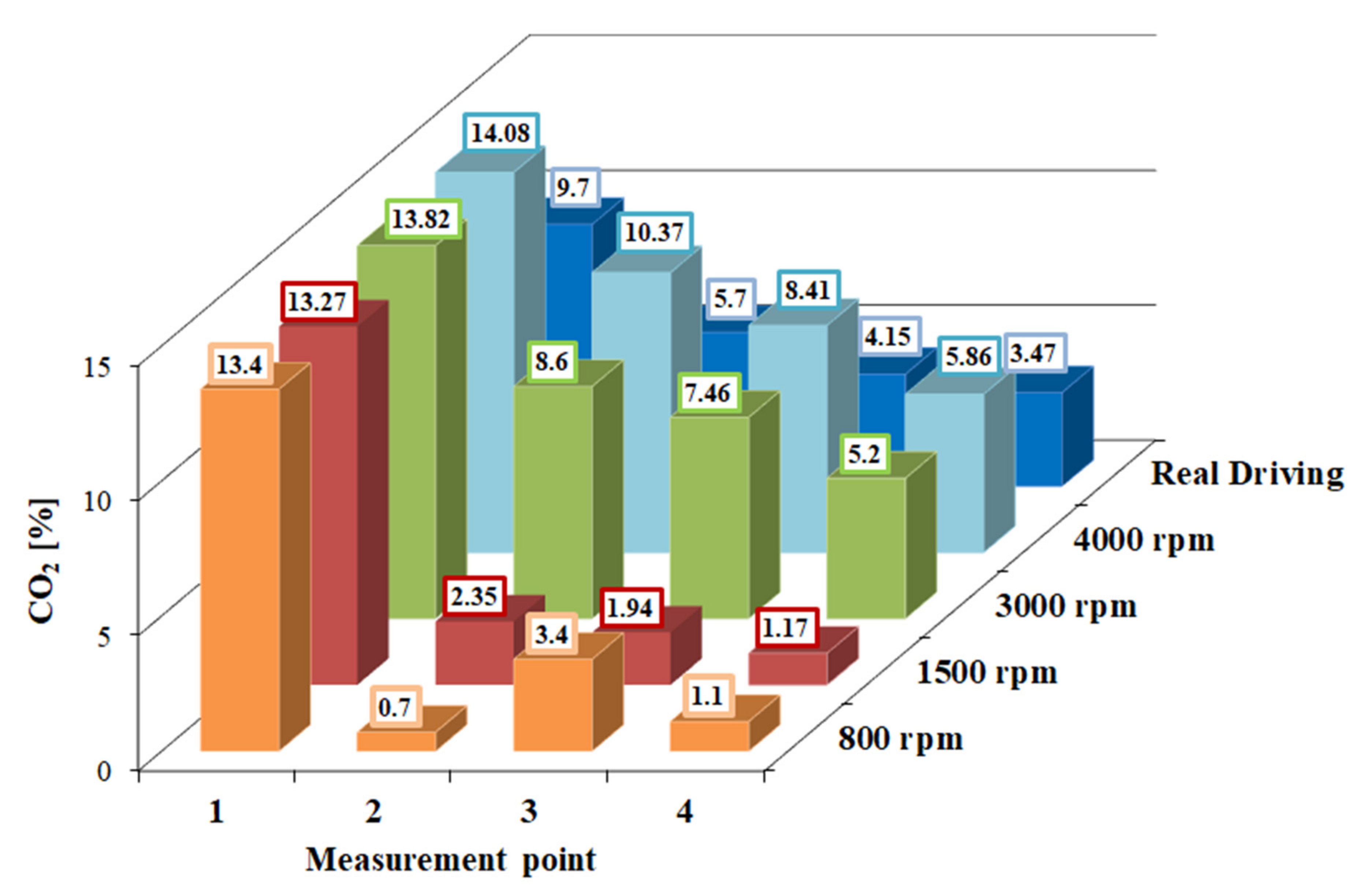
CO2 [%]	1	13.4 ± 0.6	13.27 ± 0.01	13.82 ± 0.02	14.08 ± 0.01	9.7 ± 0.12
	2	0.7 ± 0.2	2.35 ± 0.08	8.6 ± 0.1	10.37 ± 0.09	5.7 ± 0.08
	3	3.4 ± 0.2	1.94 ± 0.05	7.46 ± 0.06	8.41 ± 0.06	4.15 ± 0.06
	4	1.1 ± 0.2	1.17 ± 0.02	5.2 ± 0.1	5.86 ± 0.08	3.47 ± 0.06
CO [%]	1	0.47 ± 0.02	0.549 ± 0.002	0.463 ± 0.002	0.454 ± 0.003	0.418 ± 0.006
	2	0.057 ± 0.005	0.107 ± 0.001	0.291 ± 0.002	0.341 ± 0.003	0.214 ± 0.004
	3	0.111 ± 0.002	0.093 ± 0.001	0.261 ± 0.001	0.335 ± 0.002	0.17± 0.003
	4	0.04 ± 0.003	0.058 ± 0.001	0.19 ± 0.003	0.199 ± 0.002	0.145 ± 0.002
HC [ppm]	1	253 ± 15	157 ± 1	109 ± 1	89 ± 1	529 ± 5
	2	44 ± 2	46.5 ± 0.2	66.5 ± 0.9	63.3 ± 0.3	203 ± 2
	3	60 ± 2	37.0 ± 0.5	53.2 ± 0.3	57 ± 1	145 ± 2
	4	47 ± 3	35.5 ± 0.4	48.4 ± 0.5	49.7 ± 0.8	129 ± 2
NOx [ppm]	1	459 ± 114	255 ± 1	508 ± 18	884 ± 8	890 ± 16
	2	5 ± 2	49 ± 2	351 ± 6	657 ± 6	725 ± 24
	3	38 ± 2	28 ± 1	248 ± 8	751 ± 18	538 ± 17
	4	13 ± 1	19.5 ± 0.6	195 ± 4	381 ± 7	437 ± 13
PM [mg/m3]	1	0.6 ± 0.09	5.6 ± 0.8	3.1 ± 0.3	7.3 ± 0.1	1.45 ± 0.06
	2	0 ± 0	0.003 ± 0.002	0.4 ± 0.02	0.8 ± 0.2	0.028 ± 0.004
	3	0 ± 0	0.014 ± 0.002	0.071 ± 0.004	0.9 ± 0.3	0.035 ± 0.006
	4	0.07 ± 0.02	0.009 ± 0.003	0.22 ± 0.02	0.5 ± 0.1	0.048 ± 0.008

) were checked for significant errors, and results deemed to be incorrect as a result of errors in the measurement procedure were rejected. The statistical study allowed us to determine the measurement uncertainty, which is the basic parameter for assessing the conditions of the performed measurements. The selected vehicle was tested at four measurement points relative to its body differing in height and distance between the measuring probe and the exhaust pipe. In tests on a stationary vehicle, the concentration of harmful exhaust gas components was measured for stable engine rotational speeds maintained at 800 rpm, 1500 rpm, 3000 rpm and 4000 rpm. Then, similar measurements were carried out during the actual drive on the route covering the very center of the city.

The concentration of carbon dioxide was closely related to the position of the measuring probe, and the measured concentration of CO₂ decreased as the distance increased during the measurement (Figure 7). In the measurements behind the stationary vehicle in point 1, located directly in the exhaust pipe, the concentration of this compound for all engine rotational speeds was similar and reached 13.4–14.08%. For comparison, when measuring at point 4, the differences in carbon dioxide concentration ranged from 1.1% for 800 rpm to 5.86% for 4000 rpm.

This means that the measured compound was more dispersed at lower rotational speeds. For rotational speeds equal to 800 rpm and 1500 rpm, almost 92% of CO₂ was dispersed between the first and fourth measuring points, while for higher engine speeds (3000 rpm and 4000 rpm) this value was about 60%. In the case of carbon dioxide measurements in real operating conditions, the lowest values measured directly from the engine exhaust system were obtained (9.7%). This is due to the fact that the vehicle in motion was operated in various conditions, which was influenced, among others, by engine braking, idling and a varied acceleration profile. In the case of the farthest distance of the measuring probe from the exhaust pipe, the value (3.47%) obtained for dynamic measurements was greater than values obtained for lower engine rotational speeds and smaller than the values obtained for higher rotational speeds. According to the measurement results, 64% of the carbon dioxide emitted has been dispersed. It is also worth noting that for the measurements carried out for the rotational speed of 800 rpm, the obtained measurement uncertainty was an order of magnitude greater than in other cases. Compared to stationary measurements, the measured concentration of carbon dioxide was lower by an average of 29%.The concentration of carbon monoxide also closely depended on the position of the measuring probe, as the distance increased during the consecutive measuring points, the concentration of CO decreased (Figure 8). In stationary vehicle measurements, as in the case of carbon dioxide in point 1, the obtained values for 800 rpm, 3000 rpm and 4000 rpm were similar (0.454−0.47%), with the exception of the rotational speed of 1500 rpm (0.549%), however, this may be due to the operating conditions of the drive system; there was a global shortage of air in the combustion chamber and thus incomplete combustion of the air-fuel mixture. In probe location point 4, the lowest concentration of 0.04% was obtained for 800 rpm, while the highest value of 0.199% was achieved for 4000 rpm. This means that the compound was more dispersed at lower rotational speeds. For lower rotational speeds, about 90% of CO was dispersed between the first and fourth measuring points, while for the rotational speed of 4000 rpm and 3000 rpm, this value was 56% and 59%, respectively. In the case of the real drive measurements, the lowest value measured directly from the engine exhaust pipe was found (0.414%). While for the measuring probe being placed at the farthest distance away the value obtained for dynamic measurements (0.145%) was three times higher than the values obtained for low rotational speeds and, on average, 25% lower compared to measurements at higher engine speeds. For the measurements in real operating conditions, 65% of carbon monoxide was dispersed. In relation to stationary measurements, the concentration of carbon dioxide was lower on average by about 14%.

For the hydrocarbon concentration measurements, the highest values were obtained while the measurement sample was being drawn directly from the exhaust pipe outlet (Figure 9). In contrast to CO₂ and CO, the HC concentration value increased inversely proportional to the engine rotational speed. This is because under the conditions in which the vehicle was tested, incomplete combustion occurred to a greater extent in the combustion chamber. In addition, the research facility was produced in 1997, which means that the catalytic reactor installed in it was no longer fully operational, which had an impact on the oxidation of hydrocarbons. For measurements behind a stationary vehicle in probe point 1, for the rotational speed of 800 rpm, the value of this compound was 253 ppm, while for the rotational speed of 4000 rpm it was measured at only 89 ppm. For the remaining measurement points, the values were relatively even and reached values between 35.5 ppm and 66.5 ppm. The greatest dispersion of emitted hydrocarbons was obtained for 800 rpm (81%). For the remaining rotational speeds, the following values of dispersion were obtained—77% (1500 rpm), 56% (3000 rpm) and 44% (4000 rpm). This means that the dissipation of HC was closely related to the engine operating parameters, and the emitted gas was more dispersed at lower rotational speeds. Much higher hydrocarbon concentration values were measured when traveling in real driving conditions, however. With regard to stationary measurements for the first and second measurement probe points, this difference was on average 72%, and for the more distant probe sampling points (third and fourth), 65%. HC increased by 75% during the real drive.

The concentration of nitrogen oxides is strictly tied to the rotational speed of the vehicle engine. As the engine speed increased, the concentration of NO_x increased as well (Figure 10). In the case of tests with measurements done directly behind a stationary vehicle, the highest values were obtained for 4000 rpm regardless of the probe measuring point, while the lowest values were obtained for the lowest value of engine speed, excluding point one. It is worth noting, however, that in point one for 800 rpm, the uncertainty value measurement was 114 ppm, (for the remaining cases the measurement uncertainty was calculated to be lower than 24 ppm), hence the conclusion that the presented value for the lowest speed was highly uncertain due to the measuring equipment. The dispersion between probe position points 1 and 4 was 98% at 800 rpm, 92% at 1500 rpm, 62% at 3000 rpm and 57% at 4000 rpm, respectively. This means that the compound was more dispersed at lower rotational speeds. As for measurements in real operating conditions, the lowest values of dispersion of the analyzed exhaust compound were obtained (51%). Also, the values of the concentration of nitrogen oxides alone were the highest at almost all measurement points tested. In comparison to the stationary measurements, the NO_x concentration was on average 44% higher when measured in real conditions.

The concentration of particulate matter when measured behind a stationary vehicle strictly depended on both the position of the measuring probe as well as the rotational speed of the vehicle engine (Figure 11). As the distance increased for the consecutive measurements, the obtained PM concentration value decreased and increased with increasing vehicle rotational speed.

The conducted empirical research concerning the analysis of the harmful substances concentrations in the exhaust gas cloud behind the test vehicle equipped with a spark ignition engine was an approach to the problem of assessing exhaust emissions from moving vehicles [12,25,26,27,28,29,30,31]. The summary of the relative exhaust gas dispersion behind the vehicle for both stationary and dynamic tests was presented in

Table 5. Dispersion of the exhaust cloud behind the vehicle.

Substance	Measurement	Dispersion between Probe Points 1–2 [%]	Dispersion between Probe Points 1–3 [%]	Dispersion between Probe Points 1–4 [%]
CO2	Stationary—800 rpm	94.8	74.6	91.8
	Stationary—1500 rpm	82.3	85.4	91.2
	Stationary—3000 rpm	37.8	46.0	62.4
	Stationary—4000 rpm	26.3	40.3	58.4
	Dynamic	41.2	57.2	64.2
CO	Stationary—800 rpm	87.9	76.4	91.5
	Stationary—1500 rpm	80.5	83.1	89.4
	Stationary—3000 rpm	37.1	43.6	59.0
	Stationary—4000 rpm	24.9	26.2	56.2
	Dynamic	48.8	59.3	65.3
HC	Stationary—800 rpm	82.6	76.3	81.4
	Stationary—1500 rpm	70.4	76.4	77.4
	Stationary—3000 rpm	39.0	51.2	55.6
	Stationary—4000 rpm	28.9	36.0	44.2
	Dynamic	61.6	72.6	75.6
NOx	Stationary—800 rpm	98.9	91.7	97.2
	Stationary—1500 rpm	80.8	89.0	92.4
	Stationary—3000 rpm	30.9	51.2	61.6
	Stationary—4000 rpm	25.7	15.0	56.9
	Dynamic	18.5	39.6	50.9
PM	Stationary—800 rpm	100	100	88.3
	Stationary—1500 rpm	99.9	99.8	99.8
	Stationary—3000 rpm	87.1	97.7	92.9
	Stationary—4000 rpm	89.0	87.7	93.2
	Dynamic	98.1	97.6	96.7

. As the presented comparison indicates, the vehicle motion is beneficial in the assessment of the exhaust gases concentrations behind the moving vehicle, because the measured emission values at successive distances behind the exhaust system in most points achieve better parameters than in stationary tests (for crankshaft speeds up to 1500 rpm). The actual composition of the exhaust gases contains various chemical compounds. Their behavior in the air is similar when dispersed behind a moving vehicle, but their concentrations have different values, and the greatest observable differences occurred between NO_x and PM.

5. Conclusions

From the studies of the relative exhaust gas dispersion behind the vehicle, it is apparent that vehicle movement is beneficial in the assessment of exhaust gas concentrations behind a moving vehicle, because the measured emission values at successive distances behind the exhaust system in most points achieve better parameters than in stationary tests. The dispersion of harmful compounds in the air behind the vehicle is similar, despite the fact that their concentrations reached different values. The largest observable differences occurred in the case of nitrogen oxides and particulate matter. In stationary measurements, the impact of external wind and air movement on the measurement results has been limited. In real operation, however, this was not possible to do. Nevertheless, the meteorological conditions, which are implemented in the numerical calculations, were measured. The obtained test results were used in the simulation of exhaust gas dispersion behind vehicles with various body types in the ANSYS FLUENT software. The obtained research results presented in the article were used, among others, in the analysis of exhaust gas temperature distribution, speed, density, etc. A proper assessment of the presented test results makes it possible to extend the models for new vehicle bodies/types of vehicles as well as to simulate different operating conditions. The most important conclusion from the performed research is the confirmation that carrying out exhaust emission measurements behind a moving vehicle is indeed possible, while maintaining the appropriate distance and taking into account the phenomenon of dispersion of exhaust components (different for individual combustion products).

References

- World Health Organization. Available online: https://www.who.int/ (accessed on 21 January 2021).
- Mueller, C.J.; Nilsen, C.W.; Ruth, D.J.; Gehmlich, R.K.; Pickett, L.M.; Skeen, S.A. Ducted fuel injection: A new approach for lowering soot emissions from direct-injection engines. Appl. Energy 2017, 204, 206–220. [Google Scholar] [CrossRef]
- Gehmlich, R.K.; Mueller, C.J.; Ruth, D.J.; Nilsen, C.W.; Skeen, S.A.; Manin, J. Using ducted fuel injection to attenuate or prevent soot formation in mixing-controlled combustion strategies for engine applications. Appl. Energy 2018, 226, 1169–1186. [Google Scholar] [CrossRef]
- Dimitrakopoulos, N.; Belgiorno, G.; Tunér, M.; Tunestål, P.; Di Blasio, G. Effect of EGR routing on efficiency and emissions of a PPC engine. Appl. Therm. Eng. 2019, 152, 742–750. [Google Scholar] [CrossRef]
- Guido, C.; Beatrice, C.; Di Iorio, S.; Fraioli, V.; Di Blasio, G.; Vassallo, A.; Ciaravino, C. Alternative diesel fuels effects on combustion and emissions of an euro5 automotive diesel engine. SAE Int. J. Fuels Lubr. 2010, 3, 107–132. [Google Scholar] [CrossRef]
- Napolitano, P.; Guido, C.; Beatrice, C.; Di Blasio, G. Study of the effect of the engine parameters calibration to optimize the use of bio-ethanol/RME/diesel blend in a Euro5 light duty diesel engine. SAE Int. J. Fuels Lubr. 2013, 6, 263–275. [Google Scholar] [CrossRef]
- Buchholz, B.A.; Mueller, C.J.; Martin, G.C.; Cheng, A.S.; Dibble, R.W.; Frantz, B.R. Tracing fuel component carbon in the emissions from diesel engines. Nucl. Instrum. Methods Phys. Res. Sect. B Beam Interact. Mater. At. 2004, 223, 837–841. [Google Scholar] [CrossRef] [Green Version]
- Yang, Y.; Bernard, Y.; Dallmann, T. Technical Considerations for Choosing a Metric for Vehicle Remote-Sensing Regulations. ICCT 2019. pp. 2–14. Available online: https://theicct.org/sites/default/files/publications/China_remotesensing.FINAL_.pdf (accessed on 22 March 2021).
- Bernard, Y.; German, J.; Muncrief, R. Worldwide Use of Remote Sensing to Measure Motor Vehicle Emissions. ICCT 2019. pp. 1–23. Available online: https://theicct.org/publications/worldwide-use-remote-sensing-measure-motor-vehicle-emissions (accessed on 22 March 2021).
- Dalmann, T.; Bernard, Y.; Tietge, U.; Muncrief, R. Remote Sensing of Motor Vehicle Emissions in Paris. 2019. Available online: https://theicct.org/publications/on-road-emissions-paris-201909 (accessed on 22 March 2021).
- Tietge, U.; Bernard, Y.; German, J.; Muncrief, R. A Comparison of Light-Duty Vehicle NOx Emissions Measured by Remote Sensing in Zurich and Europe. ICCT 2019. pp. 1–29. Available online: https://theicct.org/publications/LDV-comparison-NOx-emissions-Zurich (accessed on 22 March 2021).
- Tkaczyk, M.; Sroka, Z.J.; Krakowian, K.; Wlostowski, R. Experimental Study of the Effect of Fuel Catalytic Additive on Specific Fuel Consumption and Exhaust Emissions in Diesel Engine. Energies 2021, 14, 54. [Google Scholar] [CrossRef]
- Warguła, Ł.; Kukla, M.; Lijewski, P.; Dobrzyński, M.; Markiewicz, F. Impact of Compressed Natural Gas (CNG) Fuel Systems in Small Engine Wood Chippers on Exhaust Emissions and Fuel Consumption. Energies 2020, 13, 6709. [Google Scholar] [CrossRef]
- Szymlet, N.; Lijewski, P.; Kurc, B. Road Tests of a Two-Wheeled Vehicle with the Use of Various Urban Road Infrastructure Solutions. J. Ecol. Eng. 2020, 21, 152–159. [Google Scholar] [CrossRef]
- Rymaniak, Ł.; Lijewski, P.; Kamińska, M.; Fuć, P.; Kurc, B.; Siedlecki, M.; Kalociński, T.; Jagielski, A. The role of real power output from farm tractor engines in determining their environmental performance in actual operating conditions. Comput. Electron. Agric. 2020, 173, 105405. [Google Scholar] [CrossRef]
- Merkisz, J.; Gallas, D.; Siedlecki, M.; Szymlet, N.; Sokolnicka, B. Exhaust emissions of an LPG powered vehicle in real operating conditions. In E3S Web of Conferences; EDP Sciences: Ulis, France, 2019; Volume 100. [Google Scholar] [CrossRef] [Green Version]
- Lijewski, P.; Fuc, P.; Dobrzynski, M.; Markiewicz, F. Exhaust emissions from small engines in handheld devices. In MATEC Web of Conferences; EDP Sciences: Ulis, France, 2017; Volume 118. [Google Scholar] [CrossRef] [Green Version]
- Merkisz, J.; Lijewski, P.; Fuc, P.; Siedlecki, M.; Weymann, S. The use of the PEMS equipment for the assessment of farm fieldwork energy consumption. Appl. Eng. Agric. 2015, 31, 875–879. [Google Scholar]
- Komada, P.; Wójcik, W.; Ciesięczyk, S. Absorption methods of gas consideration measurement in combustion process. In Polska Inżynieria Środowiska pięć lat po Wstąpieniu do Unii Europejskiej; Dudzińska, M., Pawłowski, L., Eds.; Polska Akademia Nauk Komitet Inżynierii Środowiska: Lublin, Poland, 2009; Volume 60, pp. 119–123. [Google Scholar]
- Serdecki, W. Badania Silników Spalinowych, 1st ed.; PolitechnikaPoznańska: Poznań, Poland, 2009. [Google Scholar]
- Katedra Inżynierii Biomedycznej DYDAKTYKA. Available online: http://www.dydaktyka.ib.pwr.wroc.pl/ (accessed on 9 December 2020).
- Paszko, M. Analiza struktur wirowych za poruszającym się autobusem miejskim i ich wpływu na opór aerodynamiczny. Autobusy Tech. Eksploat. Syst. Transp. 2016, 17, 1262–1265. [Google Scholar]
- Kulińczak, A.; Pankanin, G. Modelowanie ścieżki wirowej von Karmana przy użyciu pakietu ANSYS FLUENT. Przegląd Elektrotechniczny 2014, 90, 195–198. [Google Scholar]
- GPS Visualizer: Do-It-Yourself Mapping. Available online: https://www.gpsvisualizer.com/ (accessed on 16 February 2021).
- Fuc, P.; Lijewski, P.; Ziolkowski, A.; Dobrzynski, M. Development of a method of calculation of energy balance in exhaust systems in terms of energy recovery. In ASME International Mechanical Engineering Congress and Exposition; American Society of Mechanical Engineers: New York, NY, USA, 2017; Volume 58431, p. V008T10A047. [Google Scholar]
- Lijewski, P.; Merkisz, J.; Fuc, P. The analysis of the operating conditions of farm machinery engines in regard to exhaust emissions legislation. Appl. Eng. Agric. 2013, 29, 445–452. [Google Scholar]
- Merkisz, J.; Fuć, P.; Lijewski, P. Reduction of NOx Emission from Diesel Engines by the Application of Ceramic Oxygen Conductors. Urban Transport and the Environment in the 21st Century; WIT Press: Boston, MA, USA, 2008; pp. 355–367. [Google Scholar]
- Skrętowicz, M.; Janicka, A.; Wróbel, R.; Zawiślak, M. Evaluation of driver exposure risk on toxins emitted from exhausts engine in traffic congestion simulated conditions. In E3S Web of Conferences; EDP Sciences: Ulis, France, 2018; Volume 44, p. 00163. [Google Scholar] [CrossRef] [Green Version]
- Janicka, A.; Kot, E.; Skretowicz, M.; Wlostowski, R.; Zawislak, M. The effect of composition of syngas supplying the spark-ignition engine on the exhaust gas toxicity. Przem. Chem. 2016, 95, 1683–1686. [Google Scholar] [CrossRef]
- Sitnik, L.J.; Sroka, Z.J.; Andrych-Zalewska, M. The Impact on Emissions When an Engine Is Run on Fuel with a High Heavy Alcohol Content. Energies 2021, 14, 41. [Google Scholar] [CrossRef]
- Gis, W.; Pielecha, J.; Waśkiewicz, J.; Gis, M.; Menes, M. Use of certain alternative fuels in road transport in Poland. In IOP Conference Series: Materials Science and Engineering; IOP Publishing: Bristol, UK, 2016; Volume 148. [Google Scholar] [CrossRef] [Green Version]