1. Introduction
It is imperative to reduce carbon emissions to limit global warming from reaching dangerous levels [
1]. In the UK, the transport sector produced
million tonnes of carbon emissions in 2018, approximately 33 % of total UK carbon emissions [
2]. Within the transport sector, approximately 16 % of carbon emissions were attributed to heavy goods vehicles (HGVs), i.e., approximately 5 % of the total emissions in the UK [
3].
Conventional models of energy consumption of vehicles require the integration of the equations of longitudinal motion over drive cycles with varying speed and elevation profiles. This is a computationally expensive activity; particularly if it has to be done ‘inside’ an optimisation loop, such as for route planning, vehicle control system design and eco-driving strategies. Therefore, decarbonisation activities in the transport sector can benefit from a computationally efficient framework for vehicle energy consumption modelling.
For example, many fleet operators in the UK and abroad are trialling low carbon vehicles to reduce emissions and it is vital that industrially acceptable vehicles are both technically and financially feasible. For example, the effects of lightweighting and aerodynamic modifications of a semi-trailer on HGV fuel consumption were studied in in [
4]. Many commercially available low carbon vehicles, e.g., gas or electric [
5,
6], have significantly different specifications compared to their baseline vehicles, which are normally diesel. It is therefore important for fleet operators to understand which of their operations a certain vehicle can perform, given its fuel or battery pack capacity. This understanding is crucial to the widespread adoption and implementation of low carbon vehicles into fleet operations.
Another potential use of the proposed modelling framework is the eco-driving system, which runs a real-time optimisation and informs an HGV driver or autonomous system how to control the vehicle to minimise fuel consumption.
An advanced model predictive cruise control system that limits the fuel consumption rate and travel time between certain limits, exploiting vehicle-to-vehicle and infrastructure-to-vehicle communication, while maintaining a safe inter-vehicular distance [
7], is another potential use of the proposed computationally efficient modelling framework.
Heavy vehicles such as trucks and buses have a wide range of differing energy requirements depending on the vehicle type, payload, and drive cycle. Several methods are available to evaluate the energy consumption of a vehicle for the aforementioned applications. The simplest method is to use a simple average fuel consumption (single point calculation) usually expressed in the form of l/100 km or kWh/100 km (but can also be MJ/km, kWh/km or l/km). These values can be obtained from OEM-published data (e.g., [
8,
9]), or from real-world or dynamometer testing programmes. Others have developed this concept further by using an energy consumption value for different conditions such as average speed ranges and payload [
10,
11]. These types of models are used in a variety of applications, e.g., forecasting future uptake scenarios [
12] and in various micro- and macroscopic models [
13].
The advantages of these single point models are their ease of use, computational efficiency, and they do not require technical knowledge of vehicle technologies. However, there are significant drawbacks that preclude their use in the applications mentioned in the previous page. The primary disadvantage of using a single point model is these values are often derived from a standard or single drive cycle, requiring the vehicle to be tested in the laboratory or on-road using expensive equipment. These models do not consider varying payloads, drive cycles, and the instantaneous nature of these operations.
The next category is instantaneous fuel consumption models, providing the user the option to build vehicle models and test their performance over standard or real-world drive cycles. Several commercial software packages are available to model and analyse vehicles in terms of performance and energy consumption, such as LMS AMEsim [
14] and AVL CRUISE [
15]. A popular open source systems analysis tool is the advanced vehicle simulator (ADVISOR) [
16], developed by Argonne National Labs, created in the MATLAB and Simulink environment and used to simulate the performance of combustion engine and hybrid and electric vehicles. These tools all provide the user with a graphical interface to aid in the development of vehicle models, however, they require many parameter values and detailed knowledge of how the vehicle and subsystems operate, in order to generate realistic models.
Other instantaneous fuel consumption models exist, each with their own limitations; for example, the EcoGest tool requires 20 input parameters (e.g., vehicle and engine characteristics, transmission type, ambient temperature, road topography, etc.), and the comprehensive modal emission model requires over 50 input parameters and is based on experimental correlations from dynamometer testing [
17]. Again, the costs for testing and technical knowledge required are prohibitive. Other models exist and are similar to those described; for further details of available tools, a comprehensive review is provided in [
18]. Custom models can also be developed using MATLAB/Simulink or other proprietary software [
5,
19], however, the barrier to use is even higher due to the knowledge required to develop, calibrate and implement these models. In addition, the high computation time of such models will be a disadvantage for its use in applications such as eco-driving systems and model predictive cruise control systems, which require real-time implementation.
This article proposes a novel modelling framework to address the aforementioned modelling issues for both internal combustion engine (ICE) vehicles and electric vehicles (EVs).
The proposed computationally efficient (CE) modelling framework characterises a drive cycle into a vector, containing different indices. The drive cycle vector, along with another vector containing relevant vehicle parameters, is used to estimate the vehicle’s energy consumption for the drive cycle. This modelling framework enables the effect of different payloads to be evaluated. In its potential use by fleet operators for decision making, they can easily create typical drive cycle vectors corresponding to different routes and use them to evaluate different vehicles and technologies across various routes. Its computation efficiency will enable its potential use to design systems for eco-driving, model predictive cruise control, etc.
To evaluate the CE modelling framework, two use cases were used; an electric bus (EB) use case and a diesel HGV use case. The CE models were developed as MATLAB scripts. Baseline models of an EB from [
20] and a diesel HGV from [
5] were used. The baseline models were developed as MATLAB/Simulink models. The EB’s energy consumption was measured in-service, when it was trialled in London. The diesel HGV’s fuel consumption was measured in-service, while performing transport operations for a UK supermarket.
2. Computationally Efficient Modelling Framework
The modelling framework was developed using the following standard longitudinal equations of motion of a vehicle [
5,
21]:
Here, is the power applied to the wheels, m is the vehicle mass, a is the longitudinal acceleration, v is the vehicle speed, is the power dissipated by aerodynamic drag, is the power dissipated by rolling resistance, is the power required to ascend the road gradient, kg/m is the density of air, is the coefficient of aerodynamic drag, A is the vehicle’s frontal area, is the rolling resistance coefficient, m/s is the gravity and is the road slope.
Integrating
with respect to time gives the energy requirement for a drive cycle:
Here,
is the energy requirement and
is the drive cycle duration. In these variables, the subscript ‘DC’ stands for drive cycle. The modelling framework has two components: (1) when the simplification criterion in
Section 2.1 is met; and (2) when the simplification criterion is not met.
2.1. Simplified Calculations
The calculations in this section are for all intervals
, where the following criterion is met:
When the criterion in (7) is met, the applied wheel power, , in (1) is definitely positive. The criterion in (8) is a simplified version, where is a conservative value for the coefficient of rolling resistance.
In all such intervals, where the criterion in (8) is met, the time integral of
in (6) is rewritten as follows:
where
Here,
is the number of discretisation samples in the interval
,
is one of the four drive cycle indices, and
is defined as
Here, is the vehicle speed in sample i.
Similarly, the integrals of
and
in (6) are approximated as follows:
where
and
where
and
Here, is time in sample i, and and are two of the four drive cycle indices.
In (4),
can be rewritten as
, where
h is the road elevation. The integral of
in (6) can now be approximated as follows:
where
and
Here, is one of the four drive cycle indices; is the road elevation in sample i.
Then, a drive cycle vector,
, was created using the four drive cycle indices:
Using the drive cycle vector, the energy requirement for an ICE vehicle, when the criterion in (7) is met, can be written as follows:
where
Here, is a vehicle parameter vector.
2.2. Standard Calculations
The calculations in this section are for all intervals
, where the criterion in (8) is not met. In all such intervals, (6) is discretised as follows:
Here, is the number of samples in the interval .
2.3. Total Energy
The total energy required for an ICE vehicle is:
Dividing the energy required,
, by the energy density of fuel,
, and the average energy efficiency of the ICE vehicle,
, gives the amount of fuel required:
The average energy efficiency is optimised using data from a few drive cycles, the coefficients of aerodynamic drag and rolling resistance can be obtained from literature or from coast-down tests, the vehicle’s frontal area is taken from the vehicle’s specification, and the gross vehicle weight is entered manually as it differs depending on the transport operation.
The drive cycle vector in (21) for typical drive cycles can be stored in a memory, which can reduce the number of computations to calculate the energy or fuel requirements for different vehicles or gross vehicle weights.
2.4. EV Case
For the EV case, the CE modelling framework is similar to the ICE case. The main difference is the inclusion of regenerative braking on the energy consumption. The energy requirement for an EV when the criterion in (8) is met, i.e.,
, is calculated in the same way as described in
Section 2.1. Instead of (24), the energy requirement when the criterion in (8) is not met, i.e.,
, is calculated as follows:
where
Here, is the average energy efficiency of the EV vehicle. In (29), accounts for the energy loss when the vehicle’s kinetic energy is converted back to the battery pack’s electric energy, given the in the denominator of (31).
The total energy required for an EV is now rewritten as follows:
Here,
is calculated using (22) and
is calculated using (27). Dividing the energy required,
, by the average energy efficiency of the EV vehicle,
, gives the amount of electric energy required:
The algorithm to compute the drive cycle vector for a route is shown in
Figure 1.
The algorithm to compute the total fuel or electricity requirement for a route is shown in
Figure 2.
The reminder of this article presents accurate models of two test vehicles: a diesel lorry and an electric bus. These models were calibrated and validated using extensive field testing (described next). These models were then compared with the proposed computationally efficient models.
3. Data Collection from the Vehicles
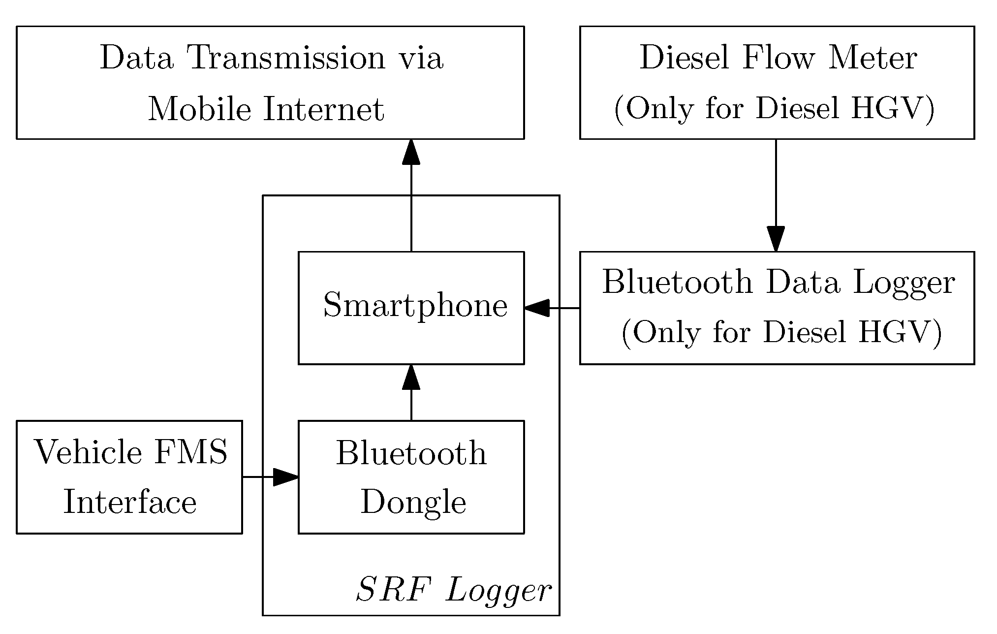
Data collection for the two use cases, i.e., the EB and diesel HGV cases, are discussed next. A block diagram of the data collection set-up is shown in
Figure 3.
A smartphone-based data logger called the SRF Logger was used for both vehicles. It also uses a Bluetooth dongle, which collects data from a vehicle’s fleet management system (FMS) port and sends them to the smartphone. This data set contains a vehicle’s throttle and brake pedal positions, vehicle speed and internal combustion engine or electric motor data. The vehicle’s GPS coordinates are collected by the smartphone.
The instrumentation on the two vehicles was the same apart from the details of the measurement of diesel or electric energy consumption (right hand side of the
Figure 3). In the EB case, the electric energy consumption data were collected directly from the EB’s FMS interface. The diesel HGV’s fuel consumption was measured using an external diesel flow meter, and sent to the smartphone using a Bluetooth data logger.
The EB was a ‘Metrocity’ manufactured by Optare Group Ltd., UK, and was trialled by a UK bus operator, Stagecoach. The diesel HGV (P320) was manufactured by Scania AB and is part of an HGV fleet operated by Waitrose Limited, UK. The data collection was done during the vehicles’ on-road commercial operations.
4. Baseline Models
The baseline energy consumption models, described in this section, were developed in Simulink.
4.1. Diesel HGV
The diesel HGV model is described in detail in [
5]. To follow a reference speed profile, the model has a Driver block. To calculate the amount of engine power, there is an Engine Power Profile block. To determine the diesel flow rate, there is an Engine Fuel Flow Rate block. To calculate the vehicle’s longitudinal equations of motion, there is a Vehicle Motion block. The Driver block controls the throttle and brake pedal inputs to follow the reference speed profile. The Engine Power Profile block calculates the engine power as a function of the engine speed and throttle input. The Engine Fuel Flow Rate block determines the diesel flow rate as a function of the engine speed and torque. For more details about the baseline diesel HGV model, see [
5].
4.2. Electric Bus
A similar baseline model was developed for an EB, which was described in detail in [
20]. This includes a
battery pack,
inverter,
electric machine,
transmission,
brake allocation,
driver and a
vehicle dynamics block. It combines the modelling works in [
21,
22]. The
battery pack discharges to operate the electric machine as a motor when the EB accelerates and charges. The electric machine operates as a generator during regenerative braking scenarios. The
inverter has a two dimensional efficiency map as a function of the electric machine’s speed and torque. The
electric machine (EM) also has a two dimensional efficiency map as a function of its speed and torque. In addition, the EM has a one dimensional peak power map as a function of its speed. The efficiency maps of the
inverter and
electric machine were obtained by scaling up the corresponding maps from the modelling work in [
22]. The energy consumption model was optimised and validated using in-service data from an EB service in London. For more details about the EB model, see [
20].
5. Evaluation Results
The EB and diesel HGV operational data were used to evaluate the accuracy and computational time of the CE modelling framework and baseline models. In both cases, the diesel or electric energy consumption predicted by the CE model and baseline models were compared against the measurements across different drive cycles. For the baseline and proposed models, their error statistics are discussed. These include the standard deviation and mean of the models’ errors with respect to the measurements.
5.1. Electric Bus Use Case
The EB’s coefficient of aerodynamic drag times frontal area was assumed to be m and the coefficient of rolling resistance was assumed to be . A gross vehicle weight of 9825 kg was considered, which includes 9000 kg of kerb weight and 11 passengers of 75 kg each. The EB’s overall efficiency was estimated to be , considering all power train components such as the electric machine and fixed gear ratio transmission.
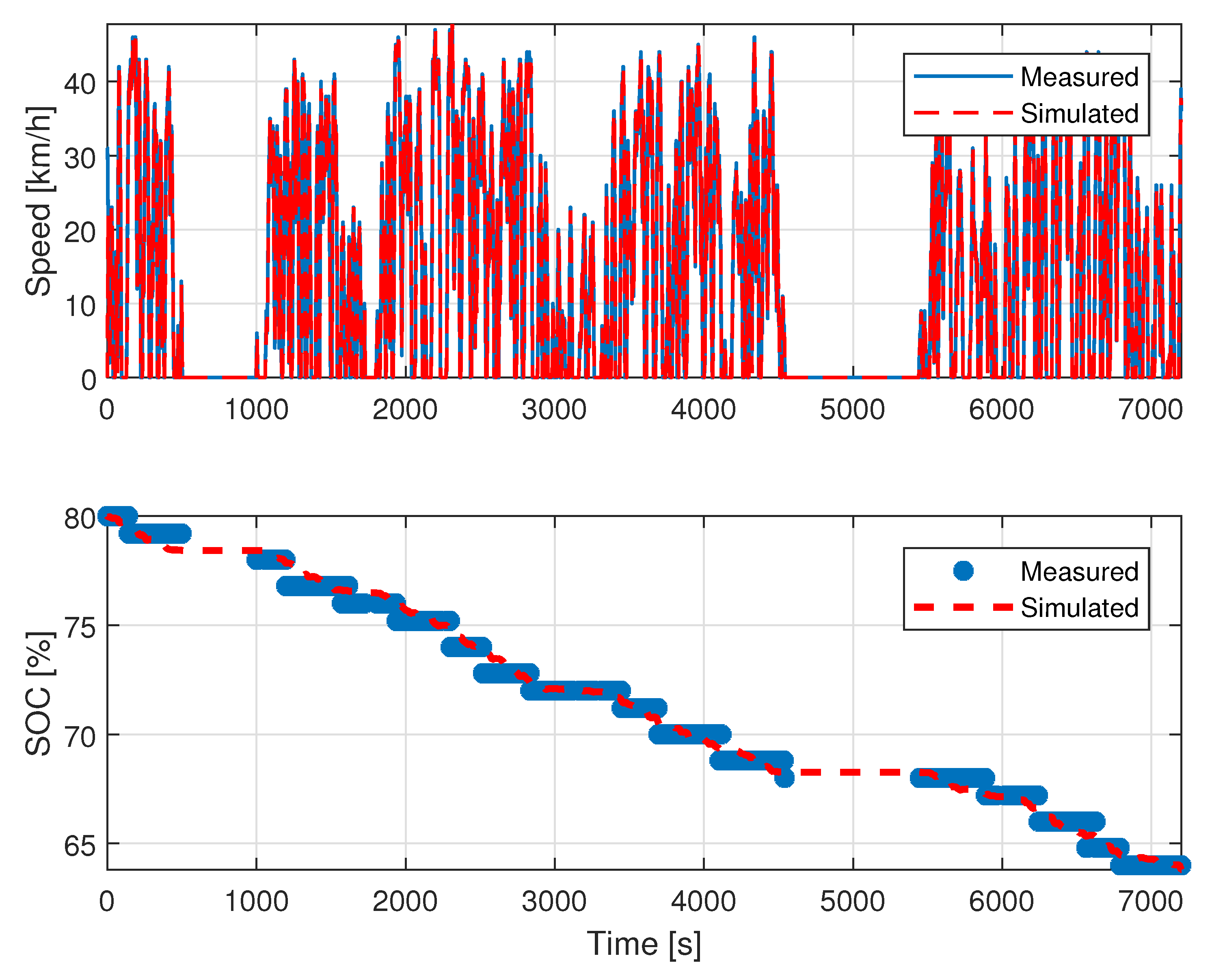
Figure 4 compares the state of charge (SOC) of the baseline EB model in [
20] against the measurements for an in-service drive cycle in London. The state of charge (SOC) indicates how much electric energy is left in the battery pack compared to its capacity and it ranges from 0% to 100%. Most commercial vehicles warn the drivers when the SOC goes below a threshold, e.g., 15%, to prevent stranding on the road. The baseline EB model input—measured speed profile—was tracked well by the model’s simulated values. In addition, for the 2 h long urban drive cycle, the baseline EB model’s SOC profile correlated well with the experimental measurements with an error less than 3%.
Figure 5 shows the energy consumption of the proposed CE model and the baseline EB model versus the measured values.
Table 1 shows the CE and baseline models’ electric energy consumption error and computation time.
e is the modelling error compared to the experimental data,
is the computation time required,
is the mean and
is the standard deviation.
The standard deviation of the EB’s CE model is %, whereas the baseline model’s standard deviation is %. The magnitudes of mean errors of both models are less than 1%. The average computation time of the baseline model is s, whereas that of the CE model is s. The results show that, without sacrificing much modelling accuracy, the CE model’s computation time is two orders of magnitude lower than the baseline model.
5.2. Diesel HGV Use Case
The diesel HGV’s coefficient of aerodynamic drag times frontal area was assumed to be
m
and the coefficient of rolling resistance was assumed to be
[
5]. The gross vehicle weight varies between 18,000 kg and 44,000 kg, depending on the payload. The HGV’s overall efficiency,
, was estimated to be
, considering all power train components such as the ICE and transmission.
Figure 6 compares the fuel consumption of the baseline diesel HGV model against the measurements for an in-service drive cycle. The baseline model input, measured speed profile, was tracked well by the model’s simulated values. The speeding event around
s may have been caused by an overtaking event when the vehicle in front slowed down due to the traffic or roundabout ahead.
Figure 6 also shows the road elevation profile. The road elevation profile in
Figure 6 was obtained using the UK Environment Agency’s Composite Digital Surface Model (DSM), available at
data.gov.uk (accessed on 24 March 2021). The road elevation profile was estimated by finding the elevation, corresponding to the vehicle’s GPS coordinates, using the DSM, which contains a LIDAR-based elevation model of more than 60% of England at 1 m spatial resolution [
23]. For the 30 min-long drive cycle, the baseline model’s fuel consumption profile correlated well with the experimental measurements with an error less than 2%.
Figure 7 shows the fuel consumption of the proposed CE model and the baseline diesel HGV model versus the measured values.
Table 2 shows the CE and baseline models’ fuel consumption errors and computation times.
The standard deviation of the CE diesel HGV model is %, whereas the baseline model’s standard deviation is %. The magnitudes of mean errors of both models are less than %. The average computation time of the baseline model is s, whereas that of the CE model is s. Similar to the EB case, these results show that without sacrificing significant modelling accuracy, the CE HGV model’s computation time is two orders of magnitude lower than the baseline model.
6. Application Case Study: HGV Routing
To demonstrate the utility of the CE modelling framework, a brief case study is presented for a hypothetical HGV fleet operator. As shown in
Figure 8, the company operates on three routes from a central depot: two of them are long haul with two stops, where the first stop intersects with the third route; the third route is regional with five stops, where the second and fourth stops intersect with the two long haul routes. In
Figure 8, LH1S1 and LH1S2 are the first and second stops on the first long haul route; LH2S1 and LH2S2 are the two stops on the second long haul route; and R1S1, R1S2, R1S3, R1S4 and R1S5 are the five stops on the regional route. Among these stops, LH1S1 and R1S2 are two names of the same stop, which lie at the intersection of the regional route and the first long haul route. Similarly, LH2S1 and R1S4 are two names of the same stop, which lie in the intersection of the regional route and the second long haul route.
Each day, based on the payload weight for each stop, the fleet operator needs to determine which of these vehicles will deliver goods at the two stops, which lie at the intersection of the regional route and long haul routes. The operator can determine the option that minimises the total fuel consumption by running an optimisation problem using the CE modelling framework. To evaluate fuel consumption for the long haul routes, the long haul drive cycle from the low-carbon vehicle partnership (LowCVP), UK, is used between each stop. The long haul drive cycle is km long. Similarly, for the regional route, the LowCVP regional delivery drive cycle is used. The regional drive cycle is km long and three regional drive cycles are combined (i.e., km long) for use between two stops of the regional delivery route.
The optimisation problem is as follows:
Here, and are the vehicles delivering goods at the two stops, which lie at the intersection of the regional route and long haul routes, 1:3 identifies the vehicle, 1: identifies the stop, is the number of stops for each vehicle, is the fuel consumption of vehicle j, is the payload weight for stop s, and d is the drive cycle type, i.e., either long haul or regional.
The use case considered three days of fleet operation and the payload weight for all the stops are shown in
Table 3. The optimisation problem was run for each day to determine at which stops each HGV should deliver goods. The optimisation results are shown in
Table 4. For the first HGV (HGV1): on day 1 and 3, the optimal stops are LH1S1/R1S2 and LH1S2, whereas on day 2, the only stop is LH1S2. Similarly, the optimisation results of the second and third HGVs (HGV2 and HGV3) can be read from
Table 4.
The optimisation problem was run using the CE modelling framework as well as the baseline vehicle model. Both methods gave the same optimised vehicle choices.
Table 5 shows the computation time for both methods. The processor used was an an Intel i7-7600 processor with dual cores of
GHz and
GHz, and with 8 GB random access memory (RAM).
Using the baseline model, on average, the optimisation problem took approximately s, whereas using the CE model, it took approximately s. In this use case, the time taken for the CE modelling framework also considered the time needed to calculate the drive cycle coefficients in (21). Even then, the optimisation problem using the CE modelling framework ran approximately 45 times faster than using the baseline model. This significant speed-up makes it possible to perform relatively accurate fuel consumption calculations within optimisation problems for route planning, control system designs, eco-driving strategies, etc.
7. Conclusions
This paper presents a computationally efficient (CE) modelling framework that can be used to model the energy consumption of both ICE and electric vehicles. The CE framework considers the specific drive cycle, vehicle and payload characteristics that are crucial in logistics and bus operations. The modelling framework is suitable to solve optimisation problems for route planning, control systems, eco-driving strategies, etc. The calculations are straightforward and do not require elaborate simulation tools.
The CE modelling framework was evaluated using the drive cycle and energy consumption data from real-world diesel HGV and EB operations in the UK, and was compared to baseline models developed in Matlab and Simulink. The models were evaluated with respect to accuracy and computational time. For the EB case, the standard deviation of the CE model’s error was 4% and mean of the CE model’s error is %. The proposed model’s mean computation time is 19 ms, which is two orders of magnitude lower than that of the baseline model. For the diesel HGV case, the standard deviation of the CE model’s error was % and the mean of the CE model’s error is %. The proposed model’s mean computation time is 17 ms, which is also two orders of magnitude lower than that of the baseline model.
Finally, a hypothetical case study was presented to illustrate the usefulness of the CE modelling framework for an HGV fleet operator to optimise their vehicle routing. In the case study, while using the CE model, the optimisation problem for vehicle routing ran approximately 45 times faster than the optimisation problem using the baseline model.


