An Integrated Approach to Adaptive Control and Supervisory Optimisation of HVAC Control Systems for Demand Response Applications

Abstract

Heating, ventilating, and air-conditioning (HVAC) systems account for a large percentage of energy consumption in buildings. Implementation of efficient optimisation and control mechanisms has been identified as one crucial way to help reduce and shift HVAC systems’ energy consumption to both save economic costs and foster improved integration with renewables. This has led to the development of various control techniques, some of which have produced promising results. However, very few of these control mechanisms have fully considered important factors such as electricity time of use (TOU) price information, occupant thermal comfort, computational complexity, and nonlinear HVAC dynamics to design a demand response schema. In this paper, a novel two-stage integrated approach for such is proposed and evaluated. A model predictive control (MPC)-based optimiser for supervisory setpoint control is integrated with a digital parameter-adaptive controller for use in a demand response/demand management environment. The optimiser is designed to shift the heating load (and hence electrical load) to off-peak periods by minimising a trade-off between thermal comfort and electricity costs, generating a setpoint trajectory for the inner loop HVAC tracking controller. The tracking controller provides HVAC model information to the outer loop for calibration purposes. By way of calibrated simulations, it was found that significant energy saving and cost reduction could be achieved in comparison to a traditional on/off or variable HVAC control system with a fixed setpoint temperature.

1. Introduction

1.1. Motivation

Increases in the cost and availability of energy as well as concerns about the environment have driven up interests in demand-based heating, ventilating, and air-conditioning (HVAC) control. Buildings are estimated to account for approximately 40% of global energy consumption ahead of other sectors, such as transportation and industry [1,2]. On average, up to 40% of the energy consumed in buildings is spent on space heating or cooling [3], and in colder climates such as Canada, this can rise to as high as 60% [4]. This significant share has sparked grid operators’ interests in numerous techniques for improving efficiency in the sector, including the concepts of carbon-neutral buildings and associated ICT tools [5], the use of advanced data-driven modelling to produce effective building digital twins [6], and also the use of advanced control and informatics concepts to improve efficiency [7]. In respect to the latter, demand response (DR) strategies offer an appealing way of reducing peak demand pressure on the grid [1]. DR techniques aim at adjusting consumers’ energy demand by incentivising energy users to reduce or eliminate non-essential usage at peak times.

A crucial factor for the successful implementation of DR strategies in buildings is the availability of flexible loads. Heating and cooling loads can be seen as flexible due to the large thermal capacity in buildings with good insulation. For example, a heat pump in combination with the thermal mass of a building can offer certain load-shifting potential without a significant compromise to occupants’ thermal comfort. However, to harness the benefits of such flexibility, existing HVAC control strategies need to be advanced. The focus of this work is upon the application of a two-step integrated control and optimisation framework for the implementation of DR in HVAC systems.

1.2. Previous Work

Certain characteristics render HVAC control different and uniquely challenging in comparison to other processes. These include nonlinear and time-varying dynamics, time-varying disturbances, and interacting and sometimes conflicting loops. In addition, many processes in HVAC systems are slow-moving with time delays. There are also constraints on the actuator rates and range limits [8], all contributing to the complexity of the HVAC control problem.

Several methods have been developed or proposed for HVAC control; however, traditional techniques such as thermostatic on/off and PID controllers are still the most widely used [9]. Other more sophisticated approaches have been found in literature, including nonlinear controller [10], robust controller [11], and soft control techniques such as those based on fuzzy logic [12] as well as on artificial neural network (ANN) [13]. A dynamic programming approach has also been suggested for the dispatch of on/off HVAC commands to achieve DR in building stock, using a hierarchical approach for multiple unit aggregation [14].

It is not uncommon to see such an HVAC control setup in hierarchical or supervisory mode. This control strategy assumes the presence of a local controller (mostly on/off type) within the heat pump which regulates the operations of its different components. The supervisory controller receives information such as room temperature and external temperature from different sensors in the building as well as energy price data and weather forecasts. This information is then processed to generate a control strategy that directs the operations of the local level controller.

Two distinct categories of supervisory control were reviewed in [15]: rule-based control (RBC) and model predictive control (MPC). RBCs usually rely on the condition of a particular trigger parameter on which a threshold is fixed. When this threshold was met, the operation of the heat pump was adjusted in a pre-planned way [15]. For example, a dynamic response controller that used a threshold price (P_th)—a piece of information specified by the consumer to adjust or maintain a setpoint was presented in [16]. If the retail price of electricity was higher than the P_th, a 1 °C step increase in setpoint temperature was applied to the thermostat at each control interval. On the other hand, when the retail price was lower than the P_th, the nominal setpoint temperature was maintained. Other HVAC applications of RBC can be found in [17,18].

The advantage of RBC lies in its simplicity since it does not require any complex models or computationally demanding algorithms. However, due to having a fixed trigger value, it is difficult for the rule-based control to adapt to changing external conditions [15]. Further, RBC lacks the ability to anticipate and optimise HVAC operation over a certain horizon. For these reasons, a control strategy based on optimisation methods such as MPC is expected to produce further improvement.

MPC has gained popularity in recent years for HVAC applications. This is because it offers solutions to some of the aforementioned challenges of HVAC control. A comprehensive review of MPC and factors affecting its performance in HVAC control (presented in [8]) showed that it performs better compared to other control methods such as classical on/off or PID control, nonlinear control, and adaptive-fuzzy-neural control. MPC can be deployed for multivariable control as well as handle time delays and actuator constraints. It also uses cost function and optimisation techniques to achieve multiple objectives. Most importantly, for the purpose of this study, MPC can be used in both local and supervisory levels of HVAC control.

At the local control level, the authors of [19] proposed a model predictive HVAC load control strategy that was aimed at reducing energy consumption as well as minimising deviations of indoor temperature from preferred values. They developed a setpoint-price assignment algorithm that captures a consumer’s attitude towards thermal comfort to determine reference temperatures for a 24 h planning horizon. Although their tests and experiments showed favourable results, the optimality of their setpoint trajectory cannot be ascertained. A simple house heating model was used in combination with electricity spot prices to evaluate the magnitude of power-saving possible through an MPC-based optimisation strategy in [20]. The focus of [21] was on the analysis of energy savings that could be achieved in a building heating system by incorporating weather predictions with MPC.

At a supervisory control level, ref. [22] trialled an HVAC control and optimisation system in two office buildings over a period of two months. They interfaced their algorithm with the buildings’ management and control systems in order to discover the most optimal power consumption schedules with respect to predicted zone conditions, comfort levels, and the weather forecast. Their control module then adjusted the supply air setpoint in accordance with the optimised power consumption schedule. A similar approach was adopted in [4], where a centralised control scheme comprising of a supervisory MPC controller and six local levels on/off controllers was deployed to reduce HVAC operating costs in a multi-zone house.

In summary, there have been multiple works concerned with HVAC control and energy management in recent years, ranging from relatively simple but sub-optimal rule-based approaches to the highly complex, nonlinear optimisation-based approaches. Very few of these control mechanisms seem to have tried to fully consider and integrate all important factors such as real-time electricity price information, occupant thermal comfort, computational complexity, and nonlinear HVAC dynamics in the context of a demand response schema in a fashion that is simultaneously scalable and industrially viable.

1.3. Current Contributions

In this work, our aim was to explore the integrated application of a digital adaptive controller and a supervisory MPC algorithm for HVAC load control. Unlike classical controllers, adaptive controllers eliminate the need to retune parameters because of changes to operating conditions and can provide predictable closed-loop behaviour for HVAC control. In the methodology that was proposed, the benefits of adaptive control were combined with those of an MPC-based optimiser. The optimiser was designed to shift the heating load (and hence electrical load) to off-peak periods by minimising a trade-off between thermal comfort and electricity costs generating a setpoint trajectory for an inner loop HVAC controller. The inner loop adaptive control provided real-time model information to the outer loop MPC supervisor to finely tune the optimisation and provided a novel integrated two-step system (with separable computational loads).

The adaptive nature of the proposed controller gave much flexibility, in that it was not restricted to any particular building type or HVAC system type. In addition, although in this work the principal focus was upon thermal control (specifically heating/cooling applications), the local control method proposed may also be applied for other related HVAC variables (e.g., humidity, airflow rate, etc.). With appropriate extensions, which will be briefly discussed, the supervisory optimisation method may also be used to regulate multiple interacting loops for demand response applications.

In order to validate and investigate the proposed approach, a number of calibrated simulations applied to a model HVAC process were presented. It was found that significant energy saving/shifting and cost reductions could be achieved in comparison to other control strategies such as rule-based thermostatic control and fixed setpoint control. It was concluded that with appropriate future development and commercialisation efforts, the method may prove to be a good candidate for a scalable, adaptable, and industrially viable integrated demand response platform for a wide variety of HVAC systems.

1.4. Structure

The rest of the paper is structured as follows. Section 2 provides a brief description of the system and the mathematical models used. It also provides necessary details of the adaptive controls, the optimisation, and the cost function and weightings employed. In Section 3, the implementation of the proposed control and optimisation scheme is presented, while Section 4 contains the results and analysis. In Section 5, the paper is concluded with recommendations for future work.

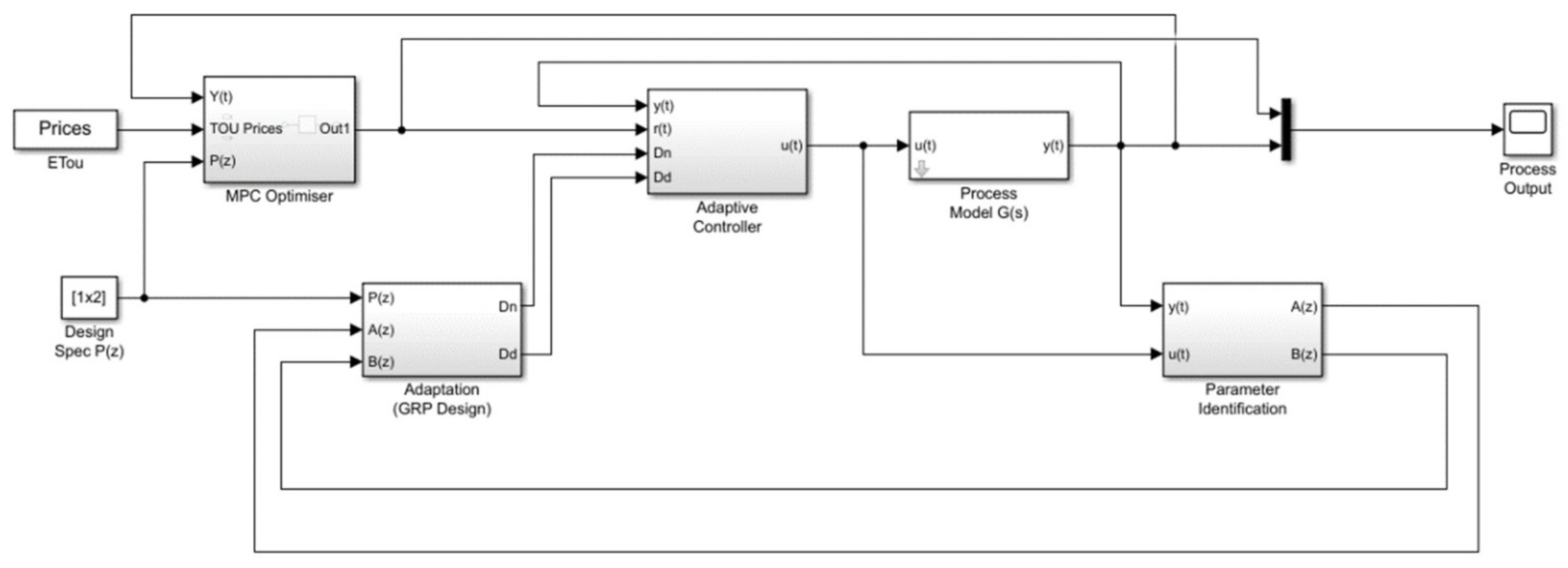
2. System Description

The supervisory control architecture used a hierarchical structure, with a supervisory optimiser at the upper level and a local digital adaptive controller. A diagram of the proposed architecture is shown in Figure 1.

The supervisory MPC was fed with (known or estimated) energy costs and measured temperature as inputs (incorporation of weather forecast information is possible and forms future work). These formed part of the objective function that was used to minimise overall energy and thermal costs over a finite future time horizon. The MPC optimiser continued iterating until a setpoint trajectory that minimises the cost functional was found. These generated setpoints were then sent to the localised adaptive controller, which in turn sent control signals to the HVAC model. Such a two-stage scheme lent itself readily to distributed environments, for example, with edge-based adaptive control in the vicinity of the HVAC zone and cloud-based implementation of the optimisation, using Internet Protocol (IP) networking and supervisory control for integration purposes [7].

2.1. HVAC Process Models

An HVAC ventilation system often comprises of different elements, including a fan, heat recovery unit, heating coil, circulating fan, valves, pipes, and ducts [6,9]. However, for the purpose of this study, our focus was principally upon heating/cooling applications, specifically the heating coil and thermal dynamics of the specific HVAC zone(s). Extensions to control of other (related) HVAC process variables were straightforward due to the ability of the controller, which was proposed to linearise a nonlinear model around specific operating points and the nature of the HVAC components themselves [6].

By applying the law of conservation of energy, up to four mathematical models of temperature changes through a heating coil could be derived (see [6,9,22]). The transfer function below represents the air-to-air temperature of a heating coil:

$$\mathrm{G}(\mathrm{s})=\frac{{\mathrm{T}}_{\mathrm{hcll}}\cdot \mathrm{s}+{\mathrm{K}}_{\mathrm{s}}}{{\mathrm{T}}_{\mathrm{hc}}\cdot \mathrm{s}+1}$$

(1)

If T_hcll = 0 in (1), and measured temperature, T, is the output of the closed loop system, then the HVAC process can be described around a local operating point by the simple first-order transfer function below [6,9]:

$${\mathrm{G}}_{\mathrm{cl}}=\frac{\mathrm{T}(\mathrm{s})}{\mathrm{R}(\mathrm{s})}=\frac{\mathrm{K}\mathrm{s}}{{\mathrm{T}}_{\mathrm{hc}}\cdot \mathrm{s}+1}$$

(2)

If the sampling time is set to ${\mathrm{T}}_{\mathrm{s}}$, the z-transform of the above transfer function can be expressed as:

$${\mathrm{G}}_{\mathrm{cl}}(\mathrm{z})=\frac{\mathrm{T}(\mathrm{z})}{\mathrm{R}(\mathrm{z})}=\mathrm{z}\left(\frac{1-{\mathrm{e}}^{\mathrm{T}\mathrm{s}}}{\mathrm{s}}\cdot \frac{{\mathrm{K}}_{\mathrm{s}}}{{\mathrm{T}}_{\mathrm{hc}}\cdot \mathrm{s}+1}\right)=\frac{\mathrm{b}{\mathrm{z}}^{-1}}{1-\mathrm{a}{\mathrm{z}}^{-1}}$$

(3)

where $\mathrm{a}={\mathrm{e}}^{{}^{-{\mathrm{T}}_{\mathrm{s}}/{\mathrm{T}}_{\mathrm{hc}}}}$ and $\mathrm{b}=\mathrm{K}\mathrm{s}\left(1-{\mathrm{e}}^{-{\mathrm{T}}_{\mathrm{s}}/{\mathrm{T}}_{\mathrm{hc}}}\right)={\mathrm{K}}_{\mathrm{s}}\cdot (1-\mathrm{a})$. Any delays present in the system (e.g., due to air transport through ducting) can be incorporated as a leading negative power of z in (3), with an additional term to capture fractional delay, if needed [6,9].

2.2. Digital Adaptive Controller

Suppose the identified HVAC system model may be presented as the general discrete transfer function, G(z) = B(z)/A(z), and the z-transform shift operator is given as $\mathrm{z}={\mathrm{e}}^{(\mathrm{\alpha }+\mathrm{j}\mathrm{\omega })\mathrm{T}\mathrm{s}}$ with sample time, T_s [23]. The digital adaptive controller was previously proposed in [24] based upon earlier work in [18]. It enables the direct propagation of a predictive controller D(z) using the preferred closed-loop pole specification, which is encoded in the polynomial P(z), if the open-loop numerator of the process (i.e., B(z) including zeros and time delay) is scaled and embedded in the closed-loop transfer function. The below controller design accomplishes the specification [23]:

$$\mathrm{D}(\mathrm{z})=\frac{{\mathrm{K}}_{\mathrm{p}}\mathrm{A}(\mathrm{z})}{\mathrm{P}(\mathrm{z})-{\mathrm{K}}_{\mathrm{p}}\mathrm{B}(\mathrm{z})},\mathrm{with}:{\mathrm{K}}_{\mathrm{p}}=\frac{\mathrm{P}(1)}{\mathrm{B}(1)}$$

(4)

To obtain the above relation, the individual equations of a process under unity negative feedback were rearranged, with the choice of scaling gain K_p made in a manner that ensures the closed-loop transfer function has unit gain and the controller contains an integrator (see [18]). Implanting the open-loop zeros of the process in the closed-loop response as presented here has many advantages, including the ability to flexibly track changes in the time delay without having to implement an elaborate delay-estimation to the polynomial B(z) and robustness against inverse response (unstable zeros) in the HVAC process [23].

The exponentially weighted recursive least squares (EW-RLS) algorithm can be used to dynamically estimate the parameters of a process model in real-time and is appropriate for use in embedded adaptive control applications without excessive model dimension [23]. The derivation of the entire EW-RLS algorithm can be found in many previous works (see e.g., [25,26]), and the main formulae for its implementation are:

$$\widehat{\mathsf{\beta }}(\mathrm{t})=\widehat{\mathsf{\beta }}(\mathrm{t}-1)+[\mathrm{K}(\mathrm{t})\times \mathrm{e}(\mathrm{t})]$$

(5)

$$\mathrm{e}(\mathrm{t})=\mathrm{y}(\mathrm{t})-[{\mathrm{x}}^{\mathrm{T}}(\mathrm{t})\times \widehat{\mathsf{\beta }}(\mathrm{t}-1)]$$

(6)

$$\mathrm{K}(\mathrm{t})=\frac{\mathrm{P}(\mathrm{t}-1)\times (\mathrm{x}(\mathrm{t}))}{{\lambda }_{\mathrm{f}}+[{\mathrm{x}}^{\mathrm{T}}(\mathrm{t})\times \mathrm{P}(\mathrm{t}-1)\times (\mathrm{x}(\mathrm{t}))]}$$

(7)

$$\mathrm{P}(\mathrm{t})=\frac{1}{{\lambda }_{\mathrm{f}}}\left[\mathrm{P}(\mathrm{t}-1)-(\mathrm{K}(\mathrm{t})\times ({\mathrm{x}}^{\mathrm{T}}(\mathrm{t}))\times \mathrm{P}(\mathrm{t}-1))\right]$$

(8)

where $\widehat{\mathsf{\beta }}(\mathrm{t})$ represents the vector of the parameter estimates of the process, y(t) refers to the current measured output of the process, x(t) is the vector of the shifted previous input and output measurements of the process being considered, K(t) is the gain vector of the estimator, P(t) represents the covariance matrix, while e(t) is the prior residual error, and ${\mathrm{\lambda }}_{\mathrm{f}}$ is the forgetting factor.

In this paper, a constant forgetting factor was implemented. At each cycle, the identification step was first executed to refresh the estimates of process parameters. Then, using Equation (3), the controller gains were determined, and the control signal was calculated and applied. This produced an effective and easily implementable method for applying the adaptive controller [23]. Preliminary test and validation results for the successful application of this adaptive controller to an HVAC thermal test facility could be found in [24].

For the purpose of setpoint optimisation, the relationship between an applied reference setpoint (e.g., coming from the MPC optimiser) r(k) and the applied control action u(k) that is output from the adaptive controller to the HVAC is of interest, as the energy consumed can be estimated as a linear product of the controller output, u(k), heater power rating ${\mathrm{W}}_{\mathrm{h}\mathrm{e}\mathrm{a}\mathrm{t}\mathrm{e}\mathrm{r}}$. Hence, the economic cost can be determined from the representative hourly electricity time of use cost ${\mathrm{E}}_{\mathrm{T}\mathrm{O}\mathrm{U}}$. Figure 2 essentially simplifies the overall control scheme shown in Figure 1. The controller output, u(k), can be determined from block-diagram algebra to be:

$$\frac{\mathrm{U}(\mathrm{z})}{\mathrm{R}(\mathrm{z})}=\frac{\mathrm{D}(\mathrm{z})}{1+\mathrm{D}(\mathrm{z})\mathrm{G}(\mathrm{z})}$$

(9)

Now, as G(z) = B(z)/A(z) and the digital controller D(z) is as described in (4), then (9) can be rewritten for the case of the adaptive control scheme as a function of the design polynomial and process parameters, as below:

$$\frac{\mathrm{U}(\mathrm{z})}{\mathrm{R}(\mathrm{z})}=\frac{{\mathrm{K}}_{\mathrm{p}}\mathrm{A}(\mathrm{z})}{\mathrm{P}(\mathrm{z})}$$

(10)

For the purpose of setpoint optimisation, the relationship between an applied reference setpoint (e.g., coming from the MPC optimiser) r(k) and the HVAC zone temperature t(k) is also of interest, as the thermal comfort is largely a function of the temperature, among several other factors such as humidity [6]. The temperature t(k) can be determined from the design principle of the controller to be a function of the design polynomial and process parameters:

$$\frac{\mathrm{T}(\mathrm{z})}{\mathrm{R}(\mathrm{z})}=\frac{\mathrm{K}\mathrm{p}\mathrm{B}(\mathrm{z})}{\mathrm{P}(\mathrm{z})}$$

(11)

Relationships (10) and (11) are of crucial importance to the configuration of the setpoint optimiser and can be provided with virtually zero overhead in real-time as a by-product of the calculations required for the controller itself, as shown in Figure 1.

2.3. MPC Objective Function

The objective function can be derived as follows. Cost of energy consumed between the current time step k over a future horizon of m steps:

$$\mathrm{E}\mathrm{c}={\displaystyle \sum _{\mathrm{k}}^{\mathrm{k}-\mathrm{m}}\max \{(\mathrm{u}(\mathrm{k})\cdot {\mathrm{W}}_{\mathrm{heater}}\cdot {\mathrm{E}}_{\mathrm{TOU}}}(\mathrm{k})),0\}$$

(12)

where the max function is used to prevent negative costs (i.e., it is assumed that heat cannot be extracted from the HVAC system and converted to electricity to be sold back to the grid). From a thermal comfort point of view, the operative temperature SP is nominally set at 22 °C. This is the ASHRAE standard recommendation [24], while the thermal cost is defined across an m-step horizon as the absolute deviation of temperature from nominal value:

$${\mathrm{T}}_{\mathrm{c}}={\displaystyle \sum _{\mathrm{k}}^{\mathrm{k}-\mathrm{m}}\left|\mathrm{t}(\mathrm{k})-22\right|}$$

(13)

The higher the absolute temperature deviation value, the higher the level of thermal discomfort felt by the occupant. Therefore, in an ideal scenario, a customer might like the overall T_c to be as low as possible. If the local controller is configured for other HVAC variable control, such as humidity, then a suitable deviation from setpoint criteria for such a variable may be used instead.

Equations (10) and (11) are employed to predict the temperature and applied controls across the prediction horizon, with the decision variables being the sequence of applied setpoints r(k). The objective function to be minimised by the MPC optimiser can therefore be stated as (14), where λ ∈ (0;1) is a weighting factor added to determine relative importance between energy cost and thermal comfort.

$$\mathrm{J}={\displaystyle \sum ((1-\lambda )\cdot {\mathrm{E}}_{\mathrm{c}}}+\lambda {\mathrm{T}}_{\mathrm{c}})$$

(14)

Since the optimisation problem is linear in the decision variables r(k), r(k + 1),…, r(k + m), linear programming can be applied for efficiently solving the optimisation problem in real-time at each time step. Once the optimisation problem is solved for the current time step, only the first reference output corresponding to r(k) is applied. The process is then repeated at the next time step to generate the next reference setpoint, in the spirit of rolling-horizon predictive control. The overall sequence of steps in the two-stage adaptive control and setpoint optimiser can be summarised as follows: (i) update estimated of plant parameters A(z) and B(z) using recursive least squares (RLS); (ii) calculate controller D(z) from these estimates and the design specification P(z); use the estimates A(z) and B(z), plus design polynomial P(z) and energy cost sequence TOU(z) to solve the setpoint optimisation and determine setpoint r(k); finally, use r(k), t(k), and D(z) to determine the control signal u(k) and apply to the HVAC system.

Although the focus in the current work was upon temperature control and its influence upon thermal comfort, MPC—by its very nature—could easily be extended to multivariable situations [27]. In the case of a more complicated thermal model, with multiple variables under local control (e.g., temperature, humidity, airflow rate), then any general convex combination of such variables may be used with an appropriate on-line convex optimiser, such as a row-action method [27]. Similarly, one may consider the case when the objective function cannot be formulated as a linear combination of two components. In such cases, the trade-off between the various (often conflicting) objectives could be studied with the Pareto multi-objective optimisation or multiplex network approaches, as usually done in biomedical models [28]. Such extensions (although relatively straightforward in the linear case) were beyond the current scope of work but are reserved for future considerations.

2.4. Simplified Case

The adaptive control and setpoint optimiser described above are general and can be used with any HVAC model and design polynomial. However, in the simpler case of a first-order HVAC model and lag-type design specification, if control law (4) is applied to the process in (3), with $\mathrm{P}(\mathrm{z})=1-\mathrm{p}{\mathrm{z}}^{-1}$ to give a controllable closed-loop lag response, then the closed loop becomes:

$${\mathrm{G}}_{\mathrm{cl}}(\mathrm{z})=\frac{\mathrm{T}(\mathrm{z})}{\mathrm{R}(\mathrm{z})}=\frac{(1-\mathrm{p}){\mathrm{z}}^{-1}}{1-\mathrm{p}{\mathrm{z}}^{-1}}$$

(15)

Then a difference equation relating temperature to setpoint changes can be written as:

$$\mathrm{T}(\mathrm{k})=\mathrm{p}\mathrm{T}(\mathrm{k}-1)+(1-\mathrm{p})\cdot \mathrm{R}(\mathrm{k}-1)$$

(16)

If parameters of A(z) are extended and substitute $\mathrm{P}(\mathrm{z})=1-\mathrm{p}{\mathrm{z}}^{-1}$ as specified earlier, Equation (16) becomes:

$$\frac{\mathrm{U}(\mathrm{z})}{\mathrm{R}(\mathrm{z})}=\frac{{\mathrm{K}}_{\mathrm{p}}[1-\mathrm{a}{\mathrm{z}}^{-1}]}{1-\mathrm{p}{\mathrm{z}}^{-1}}$$

(17)

Then a difference equation relating control signal to setpoint changes can be written as:

$$\begin{gathered} \mathrm{U}(\mathrm{z})(1-\mathrm{p}{\mathrm{z}}^{-1})=\mathrm{R}(\mathrm{z}){\mathrm{K}}_{\mathrm{p}}[1-\mathrm{a}{\mathrm{z}}^{-1}] \\ \mathrm{U}(\mathrm{k})=\mathrm{p}\mathrm{U}(\mathrm{k}-1)+{\mathrm{K}}_{\mathrm{p}}[\mathrm{R}(\mathrm{k})-(1-\mathrm{a})\mathrm{R}(\mathrm{k}-1)] \end{gathered}$$

(18)

3. Implementation

A simulation-based validation and assessment of the proposed algorithm were carried out and described in this section. Figure 3 shows the implementation of the proposed algorithm in Simulink. Parameters B(z) and A(z)—the numerator and denominator polynomials of the process model G(z)—were estimated using the recursive least squares (RLS) method. This was carried out by the block labelled parameter identification and could be set up by importing the RLS Polynomial Model Estimator block from the Simulink library and specifying the following options. The ARX model structure was preferred, and the numbers of parameters A(z) and B(z) specified were 2 and 10, respectively. Outer loop sample time was set to 15 min for setpoint optimisation, and inner loop sample time was set to 1 min for HVAC control. The forgetting factor—a value used for exponentially reducing the significance of past data at each step time—is set to 1. Forgetting factor is usually set as a value between 0 and 1, and the choice of value can affect both the speed of adaptation and the stability of the estimator [29]. Values closer to 1 produce greater stability but slower convergence in contrast to values closer to 0, which yield faster tracking but reduced stability.

Due to the transportation of fluids, gasses, or energy, HVAC systems normally have a time delay. In order to provide a calibrated, realistic analysis, an HVAC process model developed from a physical test facility was employed [30]. For a constant fan and compressor speed, an electric heater was used to control the temperature in the HVAC zone, and the following transfer function G(s) is considered as an accurate model [30]:

$$G(s)=\frac{7.2}{1+60s}{e}^{-6s}$$

(19)

In Equation (19), the time units are reported in minutes, giving a time-constant of one hour and a time delay of six minutes. The heater was fast-responding, and hence there were no rate constraints associated with the control input signal; the control input signal u(t) was amplitude constrained in the range 0–100% within the process model G(s) block in Figure 3. Experimental analysis in previous work showed that the gain, the time constant and, the time delay can vary in the real system, within range (72–84), (60–80), and (5–7), respectively [30]. Earlier work by the authors has demonstrated that the proposed inner-loop tracking controller can follow such changes and regulate the closed-loop response [24]. Hence, the purpose of the current work and experimental design was to test the performance of the integrated setpoint optimiser with the adaptive controller.

Simulation Cases

In this paper, the proposed supervisory MPC controller was tested against two other control strategies—fixed-setpoint control and rule-based thermostatic control. The fixed-setpoint strategy was adopted as the baseline method. In this case, a constant value of 22 °C was applied to the HVAC system throughout the simulation time. The aim of this was to initially evaluate baseline costs of running the HVAC when the thermostat was turned on and setpoint was fixed to the ideally preferred temperature.

In the second case, a rule-based thermostatic control strategy was deployed. For this, the average price of electricity per kWh over a 24 h period was chosen as the threshold price (P_th)—this was approximately £0.035. If the P_th was higher than the current price of electricity (E_TOU), the setpoint value of the thermostat was set to 22 °C. Conversely, if E_TOU was greater than P_th, the setpoint was adjusted to 0 °C—meaning the thermostat was turned off. This is to reduce HVAC consumption during peak times.

The proposed supervisory MPC was implemented as the third case across five different thermal comfort weight settings (i.e., when λ = 0, 0.25, 0.5, 0.75, and 1). If λ = 0, the optimiser sought to maximise energy saving at the full expense of the occupant thermal comfort, and vice versa when λ = 1. In all cases, changes to the setpoint were limited to ±3 °C from the ASHRAE recommended value of 22 °C.

To account for electricity price variations across different seasons, the performance of the supervisory optimiser at λ = 0.25 was also simulated and the results were analysed in case 3. Summary of all the test cases considered in this study can be seen in

Table 1. Summary of simulation cases for HVAC control.

Simulation Case Type	Description	Setpoint
Base	Fixed setpoint control	22 °C
Case 1	Rule-based thermostatic control	22 °C or 0 °C, depending on ETOU
Case 2	Supervisory MPC (at λ = 0, 0.25, 0.5, 0.75 and 1)	Varied, depending on λ
Case 3	Supervisory MPC (at λ = 0.25) for different seasons	Varied, depending on λ

below.

Sample electricity prices were obtained from Nord Pool Spot Market—a leading online electricity-trading platform. As discussed, the prices were interpolated at a 15 min interval over a 24 h period to correspond with the outer loop sample time. Inner loop sample time was set to 1 min.

Analysis carried out for base, case 1, and case 2 were carried out using 20 February 2019 electricity price data. Case 3 was completed using price data from 20 February, 17 April, 17 July, and 16 October 2019.

4. Results and Analysis

Base: Fixed Setpoint Control

Over the 24 h period considered, the base case (i.e., fixed-setpoint control), consumed a total of 533 KWh of electrical energy at an economic cost of £21.87 and a thermal deviation of 75 which can be considered very comfortable according to

Table 2. Thermal deviation/comfort correlation.

Thermal Deviation Range	Thermal Comfort
0–1000	Very comfortable
1000–1999	Comfortable
2000–2499	Slightly comfortable
2500–2999	Uncomfortable
3000+	Very uncomfortable

.

Case 1: Rule-Based Control

In case 1, applying a rule-based thermostatic control yielded an economic cost of £13.40 and a thermal deviation of 12,467. Energy consumption over the 24 h simulated was approximately 326 KWh. Compared to the base case, the on-off control implemented in case 1 produced an energy cost saving of £8.47 (approximately 39% less than the base case). On the other hand, a very high thermal deviation was incurred—meaning the occupant is likely to feel very uncomfortable as a result of implementing this strategy.

Case 2: Model Predictive Control

For case 2, a supervisory MPC optimisation strategy was implemented with different weight settings.

4.1. Maximum Economic Cost Saving (λ = 0)

At λ = 0, the objective of the optimiser was to minimise energy cost by producing setpoint projections that incurred the least economic cost with little regard for occupant comfort. This can be seen in effect in Figure 4. The room temperature was kept at 19 °C for most of the 24 h period considered. Overall, this helped reduce the energy consumption by 7.5% compared to the base case whilst producing a thermal deviation value that is 5397% higher than the baseline. With a thermal deviation value of 4123, the occupant could expect to feel very uncomfortable using this λ setting. The average room temperature across the 24 h period was approximately 19.5 °C.

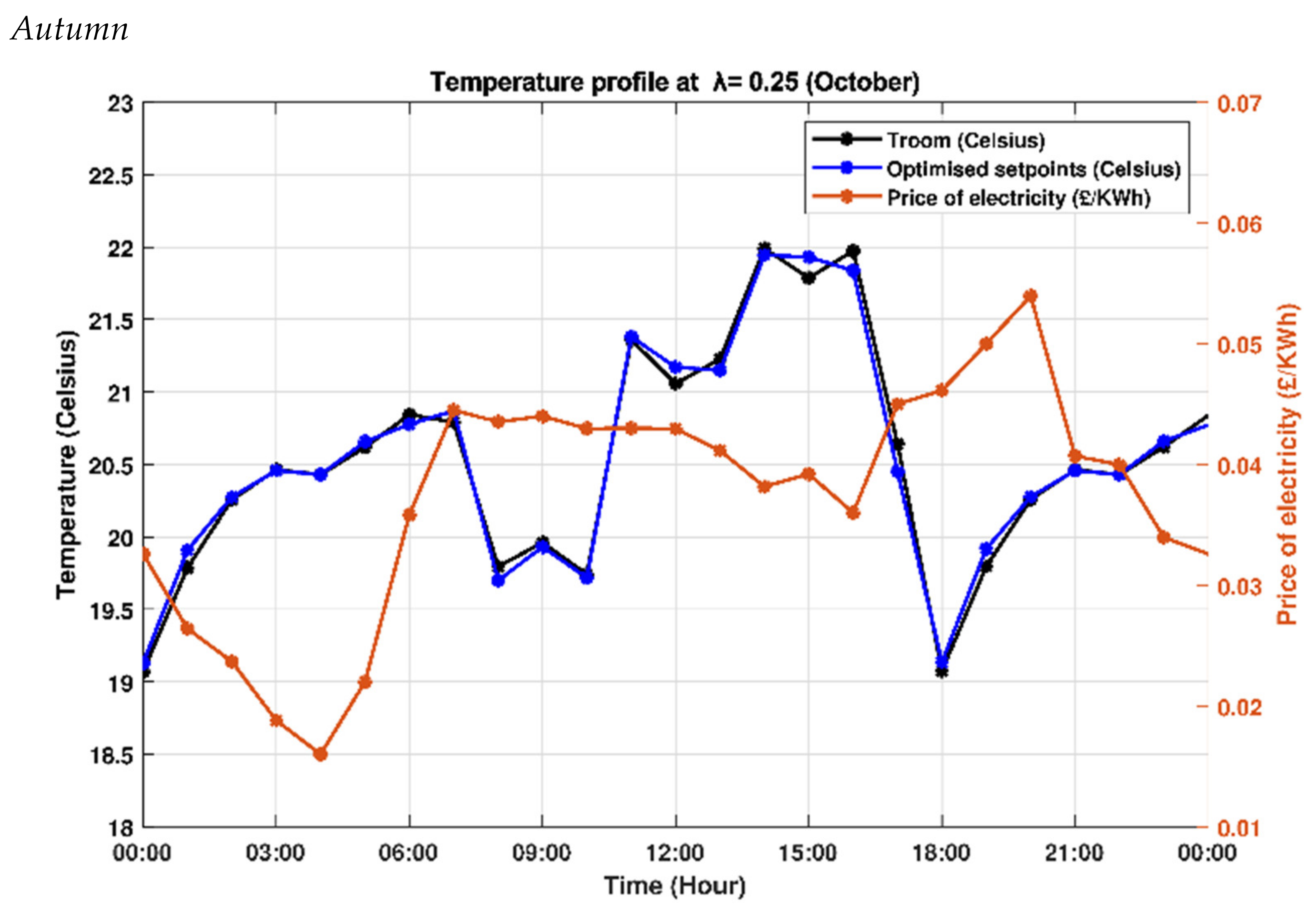
4.2. Higher Preference for Economic Cost Saving (λ = 0.25)

At λ = 0.25, the optimiser’s priority was to minimise energy cost as much as possible whilst maintaining some level of thermal comfort. As can be seen in Figure 5, the optimiser attempted to achieve this objective by keeping the setpoint close to 22 °C as much as possible during off-peak periods. Energy consumption using this λ weighting was 8% lower than in the base case, while thermal deviation increased by 3320% on the baseline value. This setting produced a thermal deviation value of 2565 and an average room temperature of 20.20 °C, which is uncomfortable (according to Table 2).

4.3. Equal Preference for Thermal Comfort and Energy Cost (λ = 0.50)

At λ = 0.50, the optimiser attempted to balance the user’s preference for good thermal comfort with careful consideration for economic cost. As can be seen in Figure 6, a fair amount of energy was consumed over the 24 h period, with the optimised setpoints kept hovering around the 22 °C mark for most of the simulation time. The economic cost incurred was £21.20—which is 3% lower than the base case. From a thermal comfort perspective, the average room temperature was 21.30 °C, at a thermal deviation of 1237.

4.4. Higher Preference for Thermal Comfort (λ = 0.75)

When λ is set to 0.75, the optimiser’s priority was to ensure good thermal comfort, by minimising thermal deviation as much as possible whilst maintaining some level of control on economic cost. From Figure 7, it can be observed that the optimised setpoint showed an insignificant deviation from the nominal value of 22 °C. This λ setting produced an average room temperature of 21.70 °C and a 1.12% reduction in energy consumption compared to the base case.

4.5. Maximum Thermal Deviation Saving (λ = 1)

In Figure 8, λ is set to 1. In this case, the occupant’s preference was to maximise thermal comfort at any cost possible. To achieve this, the optimiser ensured that the setpoint was maintained at 22 °C for the entire 24 h period considered. Since the base case (i.e., with a fixed setpoint) behaved in a similar way to the optimiser at this lambda setting, no cost-saving was produced.

A summary of the findings illustrating the trade-offs between the choice of λ, and the economic and thermal deviation is given in

Table 3. Summary of results for all three simulation cases and sub-strategies.

Simulation Case Type	Energy Consumption (KWh)	Economic Cost (£)	Thermal Deviation	Average Room Temp. (°C)	Comfortability
Base (Fixed setpoint control)	533	21.87	75	21.90	Very comfortable
Case 1 (RBC strategy)	326	13.40	12,467	13.50	Very uncomfortable
Case 2 (MPC strategy)
λ = 0.00	473	19.43	4123	19.50	Very uncomfortable
λ = 0.25	490	20.13	2565	20.20	Uncomfortable
λ = 0.50	516	21.20	1237	21.30	Comfortable
λ = 0.75	527	21.62	527	21.70	Very comfortable
λ = 1.00	533	21.87	75	21.90	Very comfortable

.

Case 3: Lambda Sensitivity vs. Seasonal Prices

For this analysis, four price data from winter to autumn were used to test the performance of the proposed optimisation algorithm. Spring, summer, and autumn results are summarised in

Table 4. Summary of results for all four seasons considered.

Season	Energy Consumption (KWh)	Economic Cost (£)	Thermal Deviation	Average Room Temp. (°C)	Comfortability
Winter	490	20.13	2565	20.20	Uncomfortable
Spring	492	18.30	2494	20.24	Slightly comfortable
Summer	492	20.86	2458	20.86	Slightly comfortable
Autumn	497	16.90	2172	20.48	Slightly comfortable

, while winter season results have already been described in Section 4.2 and Table 3 above.

Simulation results for Case 3 (summarised in Table 4) have been presented graphically in Figure 9, Figure 10 and Figure 11. From these figures, it can be seen once again that the optimiser attempted to minimise energy cost by only setting higher setpoints during off-peak periods.

5. Discussions and Conclusions

In this paper, an integrated two-step approach to demand response and demand management for HVAC systems was introduced. A supervisory model predictive controller for HVAC setpoint trajectory generation was presented. For this purpose, factors such as thermal comfort and energy cost were incorporated into a linear objective function. This setpoint optimiser was then integrated with an inner loop local adaptive controller. The performance of the supervisory MPC in conjunction with a digital adaptive controller was then tested under simulation, by varying energy and thermal deviation weightings. Trends observed suggested that, to maximise thermal comfort, λ should be kept as close as possible to 1. However, it was worth noting that this approach was not the best at saving energy costs. A sensitivity analysis illustrated that, through the choice of weighting parameter λ, trade-offs between economic cost savings and thermal comfort could be explored. Maximum saving was achieved when λ was set to 0. However, in order to save energy costs, some level of thermal comfort was being compromised. The choice of λ then lay with the end-user, bearing in mind that building occupancy can play a part in deciding what weightings to apply. For example, a λ setting of 0 may better suit a working professional who is likely to be out of the house from 8 am, while someone who works from home might prefer a setting between 0.25 and 0.5.

Again, the ability of the proposed supervisory MPC optimiser to anticipate periods of peak electricity prices and the shift heating load in order to minimise the total cost of energy used was demonstrated. This was especially evident in the setpoint trajectory produced when λ was set to 0.25. In Figure 8, higher setpoint values of 21.34 °C and 21.57 °C were prescribed for low price periods of 04:00 and 05:00, respectively, compared to the 19 °C setpoint recommended for 19:00. This load shifting capability of the optimiser is particularly useful in the demand response context; in that, it is possible to pre-arm the proposed algorithm to respond to future DR events by taking actions such as preheating, precooling, or storing heat energy for future use. A sensitivity analysis illustrated that through a choice of the weighting parameter λ, trade-offs between economic cost savings and thermal comfort could be explored.

From Table 3, it can be seen that although energy consumption in autumn was 7 KWh more than in winter, it actually costs £3.23 less to run the system in autumn than in winter. This was because of seasonal variations in energy prices. Electricity is usually costlier in winter than in another season due to the colder temperature forcing consumers to spend more time indoors. However, other factors such as extreme weather conditions, popular televised events, and so on can drive up energy demand and prices. A combination of these factors may have caused the average price of electricity sampled for summer in this study to be higher than winter’s. Nevertheless, Figure 9, Figure 10 and Figure 11 show, once again, that the optimiser anticipated periods of peak prices and adjusted setpoints to minimise energy consumption during these periods.

Although the focus of the current work was principally upon temperature control and its influence upon thermal comfort, as outlined in several places, the method could be generalised to other HVAC cases in a fairly straightforward fashion and to the multivariable case with appropriate modifications. Testing of such configurations is an area of planned work. As was also discussed previously, the proposed scheme lends itself well to a distributed computing environment, with local HVAC adaptive controls and a cloud-based optimisation scheme [7]. The exploitation of additional information related to the weather forecast, building occupancy, and visualisation of a thermal comfort/energy cost Pareto front (related to different choices of λ) is an additional area of future work. Such areas of development and future work will also extend validation and demonstration activities using more complex HVAC models in conjunction with field trials, for example, with the models and the control system developed and described in [22]. It is concluded that with appropriate future development, extensions, and commercialisation efforts, the method proposed in this work should prove to be an effective solution providing a scalable, adaptable, and industrially viable integrated demand response platform for a wide variety of HVAC systems.

References

1. Crosbie, T.; Short, M.; Dawood, M.; Charlesworth, R. Demand response in blocks of buildings: Opportunities and requirements. Entrep. Sustain. Issues 2017, 4, 271–281. [Google Scholar] [CrossRef] [Green Version]
2. Pérez-Lombard, L.; Ortiz, J.; Pout, C. A review on buildings energy consumption information. Energy Build. 2008, 40, 394–398. [Google Scholar] [CrossRef]
3. Costa, A.; Keane, M.M.; Torrens, J.I.; Corry, E. Building operation and energy performance: Monitoring, analysis and optimisation toolkit. Appl. Energy 2013, 101, 310–316. [Google Scholar] [CrossRef]
4. Afram, A.; Janabi-Sharifi, F. Supervisory model predictive controller (MPC) for residential HVAC systems: Implementation and experimentation on archetype sustainable house in Toronto. Energy Build. 2017, 154, 268–282. [Google Scholar] [CrossRef]
5. Kang, H.J. Development of an Nearly Zero Emission Building (nZEB) Life Cycle Cost Assessment Tool for Fast Decision Making in the Early Design Phase. Energies 2017, 10, 59. [Google Scholar] [CrossRef]
6. Afram, A.; Janadi-Sharaf, F. Review of modeling methods for HVAC systems. Appl. Therm. Eng. 2014, 67, 507–519. [Google Scholar] [CrossRef]
7. Short, M. Control and Informatics for Demand Response and Renewables Integration. In Handbook of Smart Materials, Technologies, and Devices: Applications of Industry 4.0; Springer Nature: Basingstoke, UK, 2021. (in press) [Google Scholar]
8. Afram, A.; Janabi-Sharifi, F. Theory and applications of HVAC control systems—A review of model predictive control (MPC). Build. Environ. 2014. [Google Scholar] [CrossRef]
9. Underwood, C. HVAC Control Systems: Modelling, Analysis and Design; Taylor & Francis/Spon: London, UK, 1999. [Google Scholar]
10. Moradi, H.; Saffar-Avval, M.; Bakhtiari-Nejad, F. Nonlinear multivariable control and performance analysis of an air-handling unit. Energy Build. 2011. [Google Scholar] [CrossRef]
11. Al-Assadi, S.A.K.; Patel, R.V.; Zaheer-uddin, M.; Verma, M.S.; Breitinger, J. Robust decentralized control of HVAC systems using -performance measures. J. Franklin Inst. 2004. [Google Scholar] [CrossRef]
12. Soyguder, S.; Karakose, M.; Alli, H. Design and simulation of self-tuning PID-type fuzzy adaptive control for an expert HVAC system. Expert Syst. Appl. 2009, 36, 4566–4573. [Google Scholar] [CrossRef]
13. Kalogirou, S.A. Artificial neural networks and genetic algorithms in energy applications in buildings. Adv. Build. Energy Res. 2009, 3, 83–120. [Google Scholar] [CrossRef]
14. Favre, B.; Peuportier, B. Application of dynamic programming to study load shifting in buildings. Energy Build. 2014, 82, 57–64. [Google Scholar] [CrossRef]
15. Péan, T.Q.; Salom, J.; Costa-Castelló, R. Review of control strategies for improving the energy flexibility provided by heat pump systems in buildings. J. Process Control 2019, 74, 35–49. [Google Scholar] [CrossRef]
16. Yoon, J.H.; Bladick, R.; Novoselac, A. Demand response for residential buildings based on dynamic price of electricity. Energy Build. 2014, 80, 531–541. [Google Scholar] [CrossRef]
17. Carvalho, A.D.; Moura, P.; Vaz, G.C.; de Almeida, A.T. Ground source heat pumps as high efficient solutions for building space conditioning and for integration in smart grids. Energy Convers. Manag. 2015, 103, 991–1007. [Google Scholar] [CrossRef]
18. Schibuola, L.; Scarpa, M.; Tambani, C. Demand response management by means of heat pumps controlled via real time pricing. Energy Build. 2015, 90, 15–28. [Google Scholar] [CrossRef]
19. Avci, M.; Erkoc, M.; Rahmani, A.; Asfour, S. Model predictive HVAC load control in buildings using real-time electricity pricing. Energy Build. 2013, 60, 199–209. [Google Scholar] [CrossRef]
20. Kajgaard, M.U.; Mogensen, J.; Wittendorff, A.; Veress, A.T.; Biegel, B. Model predictive control of domestic heat pump. In Proceedings of the 2013 American Control Conference, IEEE, Washington, DC, USA, 17–19 June 2013; pp. 2013–2018. [Google Scholar] [CrossRef]
21. Široký, J.; Oldewurtel, F.; Cigler, J.; Prívara, S. Experimental analysis of model predictive control for an energy efficient building heating system. Appl. Energy 2011, 88, 3079–3087. [Google Scholar] [CrossRef]
22. West, S.R.; Ward, J.K.; Wall, J. Trial results from a model predictive control and optimisation system for commercial building HVAC. Energy Build. 2014, 72, 271–279. [Google Scholar] [CrossRef]
23. Short, M.; Abugchem, F. On the Jitter Sensitivity of an Adaptive Digital Controller: A Computational Simulation Study. Int. J. Eng. Technol. Innov. 2019, 9, 241–256. [Google Scholar]
24. Adegbenro, A.; Short, M.; Williams, S. Development of a Digital PID-like Adaptive Controller and its Application in HVAC systems. In Proceedings of the International Conference on Innovative Applied Energy, Oxford, UK, 14–15 March 2019; Available online: https://www.researchgate.net/publication/331952706_Development_of_a_Digital_PID-like_Adaptive_Controller_and_its_Application_in_HVAC_systems (accessed on 6 April 2021).
25. De Wit, C.C.; Carrillo, J. A modified EW-RLS algorithm for systems with bounded disturbances. Automatica 1990, 26, 599–606. [Google Scholar] [CrossRef]
26. Cochrane, C.J.; Lenahan, P.M. Real time exponentially weighted recursive least squares adaptive signal averaging for enhancing the sensitivity of continuous wave magnetic resonance. J. Magn. Reson. 2008, 295, 17–22. [Google Scholar] [CrossRef]
27. Camacho, E.F.; Bordons, C. Model Predictive Control, 2nd ed.; Springer: London, UK, 2007. [Google Scholar]
28. Angione, C.; Conway, M.; Lió, P. Multiplex methods provide effective integration of multi-omic data in genome-scale models. BMC Bioinform. 2016, 17, 257–269. [Google Scholar]
29. Short, M.; Rodriguez, S.; Charlesworth, R.; Crosbie, T.; Dawood, N. Optimal Dispatch of Aggregated HVAC Units for Demand Response: An Industry 4.0 Approach. Energies 2019, 12, 4320. [Google Scholar] [CrossRef] [Green Version]
30. Bai, J.; Zhang, X. A new adaptive PI controller and its application in HVAC systems. Energy Convers. Manag. 2007, 48, 1043–1054. [Google Scholar] [CrossRef]
Figure 1. Supervisory model predictive control (MPC) plan showing a detailed breakdown of the inner loop adaptive controller. The MPC optimiser continued iterating until a setpoint trajectory that produced the least cost was found. These generated setpoints were then sent to the localised adaptive controller, which in turn sent control signals to the heating, ventilating, and air-conditioning (HVAC) model.
Energies 14 02078 g001
Figure 2. Basic closed loop representation of Figure 1, showing the inner loop digital adaptive controller D(z) and the controlled process G(z), where U(z) is the controller output.
Energies 14 02078 g002
Figure 3. Simulink implementation of the supervisory control and optimisation scheme.
Energies 14 02078 g003
Figure 4. Room temperature and MPC-generated setpoints over 24 h when λ is set to 0—indicating maximum preference for energy saving.
Energies 14 02078 g004
Figure 5. Room temperature and MPC-generated setpoints over 24 h when λ is set to 0.25—indicating higher preference for energy saving with some consideration for thermal comfort.
Energies 14 02078 g005
Figure 6. Room temperature and MPC-generated setpoints over 24 h when λ is set to 0.5—indicating balanced preference for energy saving and thermal comfort.
Energies 14 02078 g006
Figure 7. Room temperature and MPC-generated setpoints over 24 h when λ is set to 0.75—indicating a higher preference for thermal comfort with some consideration for energy cost.
Energies 14 02078 g007
Figure 8. Room temperature and MPC-generated setpoints over 24 h when λ is set to 1—indicating maximum preference for thermal comfort.
Energies 14 02078 g008
Figure 9. Room temperature and MPC-generated setpoints over 24 h using sample spring season price data.
Energies 14 02078 g009
Figure 10. Room temperature and MPC-generated setpoints over 24 h using sample summer season price data.
Energies 14 02078 g010
Figure 11. Room temperature and MPC-generated setpoints over 24 h using sample autumn season price data.
Energies 14 02078 g011