Article

Remaining Useful Life Prediction of MOSFETs via the Takagi–Sugeno Framework

Institute of Control and Computation Engineering, University of Zielona Góra, 65-246 Zielona Góra, Poland
*
Author to whom correspondence should be addressed.
Energies 2021, 14(8), 2135; https://doi.org/10.3390/en14082135
Submission received: 17 March 2021 / Revised: 8 April 2021 / Accepted: 9 April 2021 / Published: 11 April 2021
(This article belongs to the Special Issue Advanced Control Design and Fault Diagnosis)

Abstract

:
The paper presents a new method of predicting the remaining useful life of technical devices. The proposed soft computing approach bridges the gap between analytical and data-driven health prognostic approaches. Whilst the former ones are based on the classical exponential shape of degradation, the latter ones learn the degradation behavior from the observed historical data. As a result of the proposed fusion, a practical method for calculating components’ remaining useful life is proposed. Contrarily to the approaches presented in the literature, the proposed ensemble of analytical and data-driven approaches forms the uncertainty interval containing an expected remaining useful life. In particular, a Takagi–Sugeno multiple models-based framework is used as a data-driven approach while an exponential curve fitting on-line approach serves as an analytical one. Unlike conventional data-driven methods, the proposed approach is designed on the basis of the historical data that apart from learning is also applied to support the diagnostic decisions. Finally, the entire scheme is used to predict power Metal Oxide Field Effect Transistors’ (MOSFETs) health status. The status of the currently operating MOSFET is determined taking into consideration the knowledge obtained from the preceding MOSFETs, which went through the run-to-failure process. Finally, the proposed approach is validated with the application of real data obtained from the NASA Ames Prognostics Data Repository.

1. Introduction

Power Metal Oxide Field Effect Transistors (MOSFETs) are electronic components that are common in a wide range of applications, such as power conversion devices, low-voltage motor controllers, consumer electronics, automotive electronics, communications and radar systems [1,2,3]. The large number of applications of MOSFETs signifies that their durability implies the service life of many systems in which they are used. In the literature, many methods that enable the diagnosis of both individual MOSFETs and the entire systems they are composed of can be found [4,5,6]. These methods enable the fault detection of a diagnosed system and, consequently, its appropriate replacement.
Apart from the above facts, the research results presented in this paper are motivated by a wide application of MOSFETs in such systems as in, e.g., DC-DC converters [3], wind turbines [7,8], fuel injectors [9], buck converters for photovoltaic panels [10], etc. Thus, the knowledge about MOSFETs’ current health status is of paramount importance for the entire system reliability. Due to the fact that MOSFETs are a part of many devices that are critical for the safety of systems and/or their users, there is an increasing need for predicting their time to failure. Such knowledge allows an early replacement of a system component before its failure. To settle such a challenging issue, a mechanism of efficient prediction of components’ Remaining Useful Life (RUL) is required [11,12]. Thus, the methods of modeling system degradation processes largely determine the effectiveness of the RUL mechanism. There are many methods of modeling this process in the literature, among them knowledge-based models [13], life expectancy models [14], artificial neural networks [15], physical models [16] and an exponential degradation model [17,18] can be mentioned.
One of the most often used scheme for RUL prediction is based on the exponential degradation model [17,18]. All of the exponential degradation model-based methods, despite some advantages, have one common weakness, which is the lack of using historical data when diagnosing the current state of the system. Such historical data correspond to the run-to-failure of different components of the same type. Indeed, as can be seen in many publications [18], the exponential model was designed on the basis of data from one system without taking into account historical data from other systems with the same structure. To solve such a challenging problem a new methodology for RUL prediction of power MOSFETs is proposed. It is composed of two layers. The first one is based on fitting the exponential model to the on-line data and predicting RUL. In the second layer, the multiple-model Takagi-Sugeno (T-S) [19,20,21] approach for degradation modeling of power MOSFETs was developed. The proposed approach is used as a data-driven approach [8,22], which works on the basis of historical data collected from a run-to-failure dataset of MOSFETs with the same specification. Finally, the closest historical model is matched to the currently operating MOSFET. Thus, remaining useful life is predicted by the historical model. Thus, the main contributions of the paper can be summarized as follows:
  • Development of a Takagi–Sugeno framework for modeling MOSFET degradation modeling based on run-to-failure historical data. Thus, instead of a large amount of historical data, parameters of the historical models are stored.
  • Development of an on-line estimation and inference scheme selecting a historical model that is used for RUL prediction purposes.
  • Development of an on-line approach for estimating an analytical exponential model along with RUL prediction.
  • Merging together Takagi–Sugeno data-driven and analytical approaches to form an interval of RUL instead of a point prediction.
  • Experimental validation of the proposed approach based on the NASA Ames Prognostics Data Repository [23].
The paper is organized as follows. Section 2 provides background information on the construction of MOSFETs and the potential causes of their failures. Moreover, the main concept of RUL prediction and methods of MOSFETs’ degradation process modeling are described. Section 3 presents the proposed multiple model-based T-S framework for the MOSFETs’ degradation process modeling and RUL prediction. Section 4 exhibits the validation results concerning the proposed framework applied to real data obtained from the NASA Ames Prognostics Data Repository [23]. Finally, Section 5 is devoted to conclusions.

2. RUL Prediction of Power MOSFETs

2.1. MOSFETs

Power MOSFETs are one of the most commonly used semiconductor components in switching mode power supply systems. An advantage of such components is high frequency switching. Moreover, the structure of power MOSFETs ensures that they can handle a large amount of power. The design of such semiconductor devices allows using them, among others, in electrical motor drivers where high-speed switching and durability to a high current are very important. It is worth emphasizing that high voltage MOSFETs have a different structure than the typical ones. The power MOSFETs have a vertical structure, unlike typical MOSFETs (cf. Figure 1). This results in a vertical direction of channel current flow. Moreover, the N-layer is divided into two more layers, which are doped with high and low concentrations, to be able to withstand a high forward voltage. The power MOSFETs, like any other technical devices, are prone to failure. Typical failures of such systems are due to their natural limitations:
  • Maximum drain to source voltage: a nominal parameter of MOSFETs; exceeding the limit voltage results in an uncontrolled mode conduction.
  • Maximum drain current: in general, a drain current should not reach a border value. However, there are momentary increases in the current, which are called a pulse of drain current.
  • Maximum temperature: specifies the maximum temperature of the junction, which does not affects changes of functionality.
  • Gate oxide breakdown: a decrease in gate dielectric thickness causes an increased frequency of switching. A significant reduction of lifetime is noticeable when the nominal gate voltage is exceeded, which possibly results in a failure.
Taking into account the above discussion along with the practical importance of MOSFETs, it is evident that the development of new efficient RUL prediction methods is of paramount importance both from practical and theoretical perspectives. Thus, the objective of the next part of this paper is to settle such a challenging problem.

2.2. RUL Prediction Concept

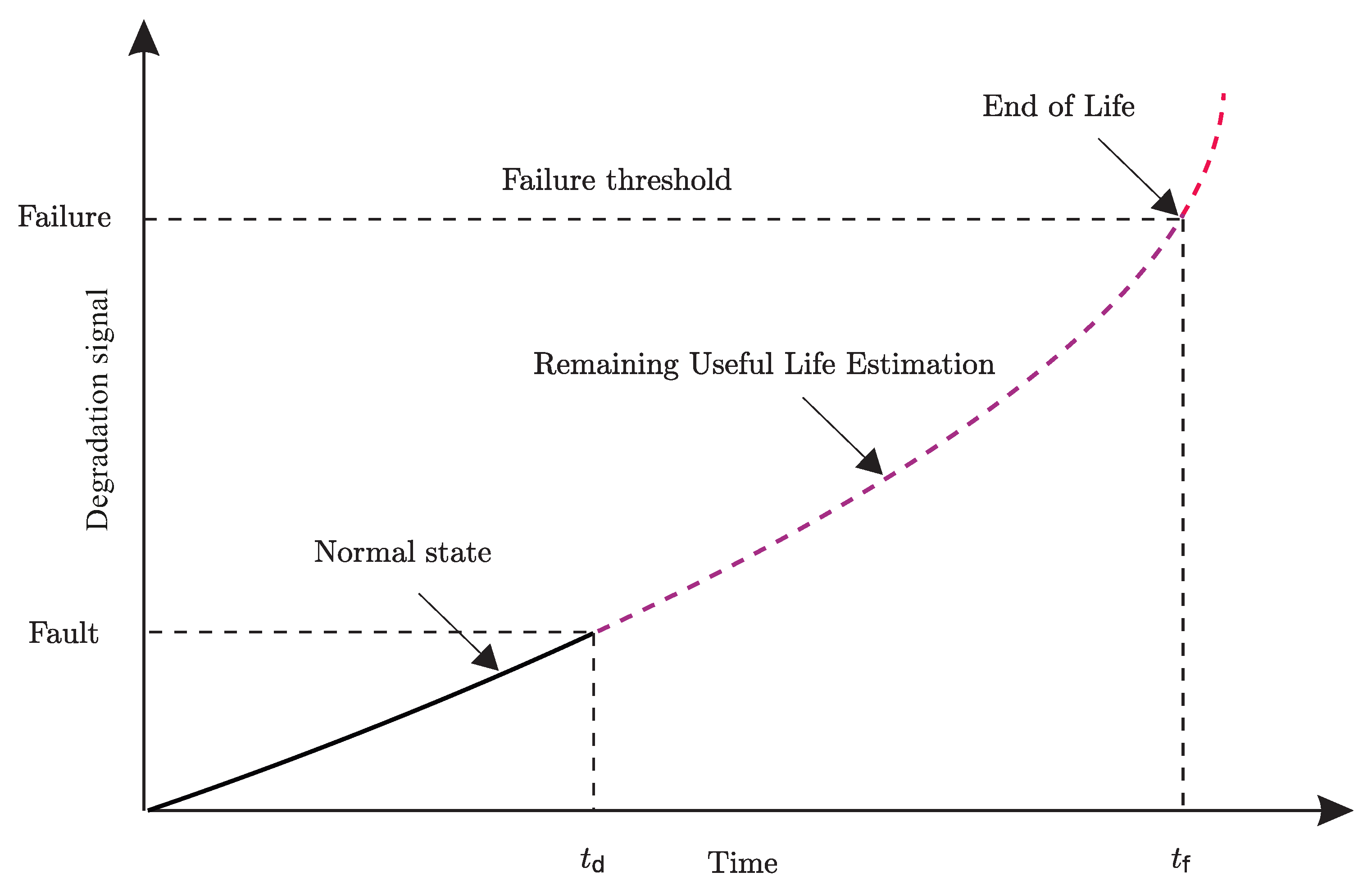
Numerous and important practical applications of power MOSFETs and their great importance for the safety of other systems make it necessary to develop new RUL prediction methods of such components. According to the diagram presented in Figure 2, power MOSFETs start operating in a faulty mode when the selected degradation signal crosses the fault threshold. This situation occurs at time t d .
This fault may be caused by a natural aging process or by the destructive influence of various external factors. The occurrence of a fault does not have to mean that the system is completely unable to work, but it may mean a decrease in its effectiveness. If the factors that caused the fault still affect the system, it may lead to its complete failure. This means that the system is unable to work. Such a state is usually called End of Life (EoL). Thus, the RUL can be perceived as the time from fault detection t d to EoL at time t f .
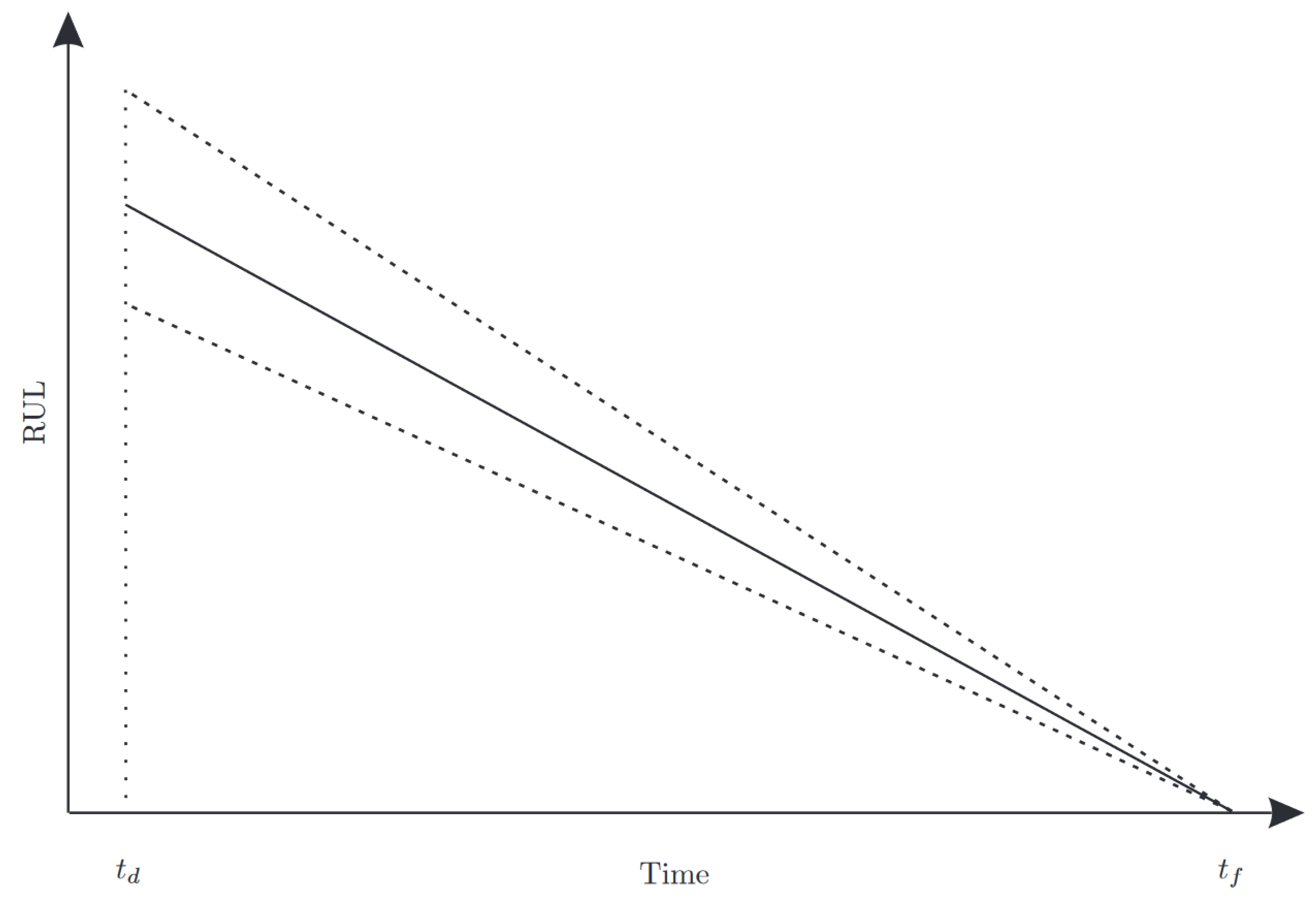
The aim of the paper is to propose a methodology enabling RUL prediction of the MOSFETs, and in particular, the determination of the so-called Time-To-Failure (TTF), which is an estimate of the time remaining until the system fails. Figure 3 presents the concept of the RUL prediction. The TTF is calculated from the time of fault detection t d to EoL at time t f . During the RUL prediction process, the accuracy of the RUL increases as the TTF decreases. This phenomenon is illustrated by decreasing the uncertainty interval of the RUL while approaching t f .
The idea of the proposed data-driven RUL prediction method is based on the application of a group of T-S models representing MOSFETs subjected to a degradation process. These models were obtained using the NASA Ames Prognostics Data Repository [23]. These data were generated using 42 power MOSFETs subject to thermal stress accelerated aging. Subsequently, the obtained T-S models can be used for health assessment of the currently monitored MOSFET. When a fault is detected in the MOSFET, the RUL prediction phase of the component being diagnosed is initiated. The proposed mechanism relies on the comparison of the currently tested MOSFET with information gathered during the training process, and the closest T-S degradation model is chosen. Then, the remaining useful life prediction is carried out and TTF is determined with the application of the developed approach. The scheme of the proposed approach is illustrated in Figure 4. The objective of the next part of this paper is to provide a comprehensive description of this scheme.

2.3. Methods of Modeling MOSFET Degradation Process

Each modeling process requires representative data that describe the behavior of a given system. These data should reflect the range of MOSFETs produced during the manufacturing process and the aging process. Accelerated aging is one of the best opportunities to collect necessary data. This method allows preparing reliable information about components without long-term reliability tests. This significantly reduces the time required to start prognostic steps. Based on collected data, it is possible to develop prognostic models. Figure 5 presents the scheme of an exemplary aging system, which consists of two power MOSFETs. The first semiconductor operates under nominal parameters while the second one is under thermal stress to accelerate aging. The use of two transistors enables continuous comparison of values and determination of the end of the aging.
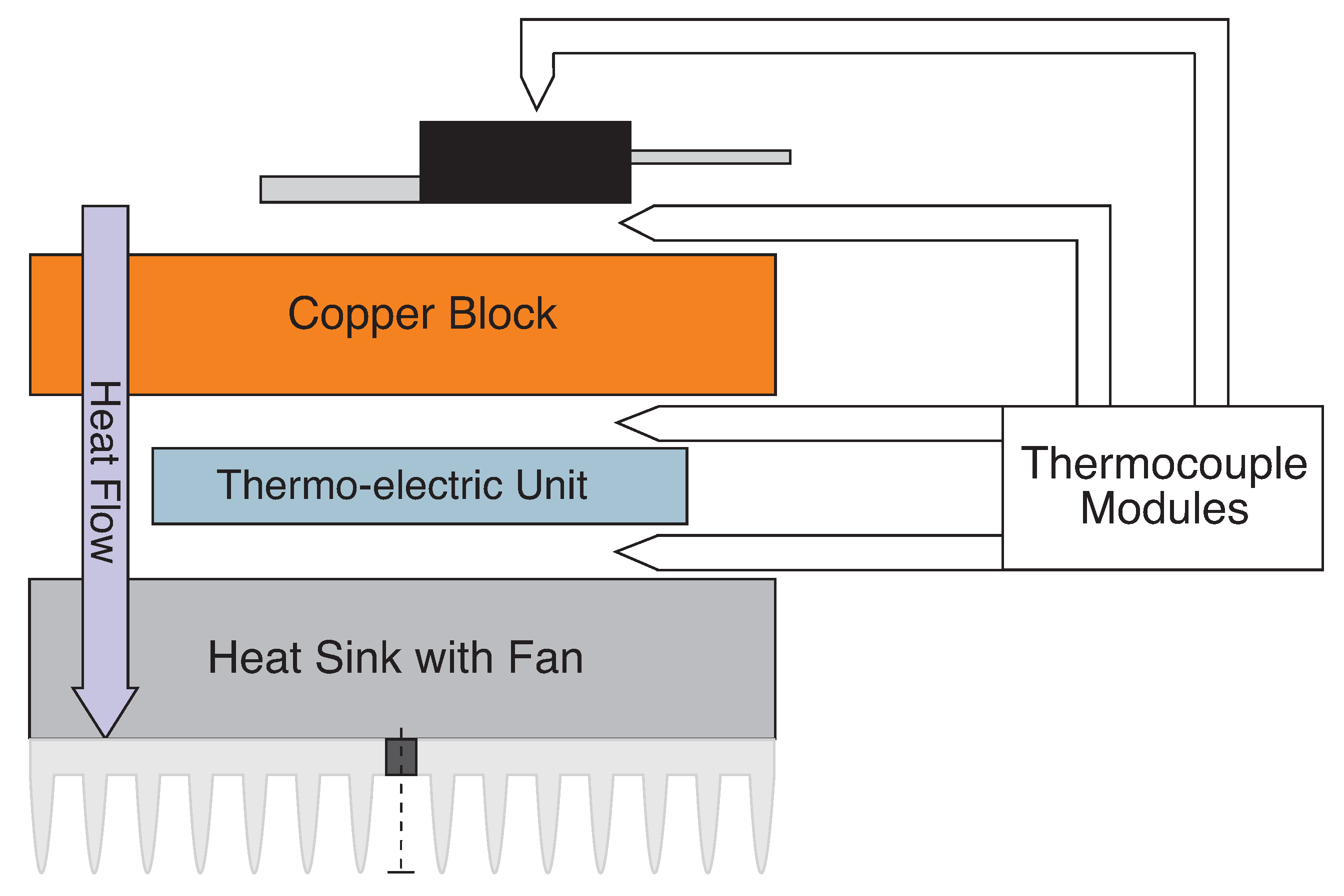
In the literature, there are two main groups of methods used for accelerated aging, i.e., temperature-based and radiation-based [24,25]. The temperature-based accelerated aging method requires a specific device to control and apply a given temperature. This type of aging is often used to accelerate aging of electronics components in Prognostics and Health Management (PHM) systems. However, the best solution is to use a thermal block (cf. Figure 6), which allows controlling the temperature of a tested device and the its flow with a given temperature. This aging process results in increased drain-source ON-state resistance ( R O N ), which may lead to de-lamination and bond-wire cracking at the source terminal.
The second method used to accelerated aging is based on a radiation effect on power MOSFET functionality [24]. In such a case, two dosage rates of radiation are used during tests. The first one has a value equal to 1.0 krad/day and it is called a low dosage rate. The second dosage rate is a higher one (3.3 rad/s), and it equals about 285 krad/day. The application of the radiation-based approach results in decreasing the voltage threshold and as a consequence a reduction of mobility as caused by oxide trapped charge and interface charges.
One of the key elements of the designed RUL prediction system is to have appropriate MOSFETs degradation models. There are several methods of system degradation modeling in the literature, including knowledge-based models [13], life expectancy models [14], artificial neural networks [15,26,27] and physical models [16].
Among the knowledge-based models the expert systems-based [28] and fuzzy rules [29] models can be distinguished. Expert systems are advisory systems, which correspond to the knowledge of human experts in a given field. They are based on collected and analyzed experiences that are applied to the system in the form of IF–THEN rules. The main weakness of this solution is in the completeness of the gathered knowledge base. Any lack of information may result in an incorrect system reaction under given operating conditions. For this reason the knowledge database in expert systems should be constantly updated and maintained. Unlike expert systems, which are based on true or false statements, fuzzy logic systems are based on intertwine rules. Contrarily to expert systems, the rules in fuzzy logic are imprecisely designed to enable a gradual membership to them. Fuzzy logic as well as expert systems are also based on knowledge databases. By using only a few appropriate fuzzy rules, it is possible to describe the modeled system better than when using the much larger number of rules used in expert systems. Moreover, using fuzzy logic systems, it is possible to obtain results even when data are incomplete and inaccurate. As in the case of expert systems, the weakness of a fuzzy rule-based approach is the need for having a complete knowledge database about the modeled system. Moreover, an appropriate reasoning mechanism is required.
The life expectancy model relies on the determination of the systems’ components’ RUL with respect to the expected risk of deterioration for assumed operating conditions. This class of methods can be divided into stochastic models [30] and statistical models [31,32]. Stochastic models, among which one can specify Bayesian networks [33], Markov models [34,35], Bayesian techniques [36,37] and Kalman filters [38,39], are based on probabilities of failure of the system at a given time. The main assumption is that the TTF for the same systems should be the same, and hence, it can be described by a probability density function. Unfortunately, the accuracy of TTF estimates depends on the population and rarity of failures. In other words, the considered failures must be statistically independent and identically distributed [40]. If there is a small amount of data related to a failure in the population, then the stochastic model will not function properly. Moreover, in case of such methods a large amount of data is necessary to create the model. Stochastic models, among which one can specify trend extrapolation methods [41,42] and Autoregressive-Moving Average (ARMA) models [43,44], are based on the trend analysis of system parameters or outputs, which are correlated with the system RUL. The disadvantage of these methods is their susceptibility to varying operating conditions that affect the measured values but are not related to system failure. Moreover, a large amount of data for model construction and validation is required.
Artificial Neural Networks (ANNs) [45,46,47] belong to another class of methods that can be used in system degradation modeling tasks. Artificial neural networks, such as neuro-fuzzy networks [48], belong to the class of so-called black-box modeling approaches. Models of this type are only intended to reflect the behavior of the modeled system degradation process. The techniques of this type are especially attractive for modeling complex and dynamic degradation processes. Unfortunately, the effectiveness of ANNs in system degradation modeling tasks depends on the representativeness of the data used during their training.
Physicals models-based approaches [49] are used when the analytical model describing the physical behavior of the degradation processes is known. Such behavior is usually described by a series of dynamic ordinary or partial differential equations. Physical models applied in RUL prognosis require the identification of at least one parameter, which can specify the system. The disadvantage of modeling the degradation process using physical models is the fact that detailed and complete knowledge about system behavior must be delivered.

3. Multiple Model-Based T-S Framework MOSFET Degradation Modeling

The weaknesses and limitations of the methods presented in Section 2.3 indicate the necessity for developing a new method for modeling MOSFETs’ degradation processes. Let us start with the exponential model description, which will be exploited in both analytical and fuzzy logic RUL layers. Exponential models belong to the group of the most often applied models [50,51]. As was already mentioned, the concept of the proposed approach relies on a combination of exponential models and a fuzzy logic framework.
At the beginning the following general form of exponential degradation model presented in [17,18] should be recalled:
x k = ϕ + θ k exp ( β k t k + σ k B ( t k ) σ k 2 2 t k ) ,
where x k denotes the modeled degradation systems parameters, such as the drain-source ON-state resistance R O N (cf. Section 2.3), ϕ is the minimum value of x k , whilst unknown parameters β , σ and θ describe the behavior of the system degradation model. Moreover, t k represents time in sample k, and σ B ( t k ) signifies a Brownian motion with the following properties N ( 0 , σ 2 t k ) . The model defined above can be transformed into a classical logarithmic notation:
z k = ln ( x k ϕ ) = ln ( θ k ) + ( β k σ k 2 2 ) t k + σ k B ( t k ) ,
and subsequently to the following compact regressor form:
z k = r k T p k ,
where r k = [ 1 , t k ] T R 2 and p k = [ ln ( θ ) , β σ 2 2 ] T R 2 are the regressor and a time-varying parameter vector, respectively.
There are many methods detailed in the literature to estimate the parameter p k . Among them, methods based on the Bayesian approach can be mentioned [17]. The main weakness of such an approach is that the initial conditions of the estimation process are not specified. Indeed, if x k is below a certain fault-free level then there is no need to update p k , as the model has close-linear properties. To overcome this limitation, Li et al. [18] introduced suitable improvements. However, the proposed approach is characterized by the disadvantages of the original method [17], which did not use historical data for different run-to-fail elements of the same type. In order to solve such a problem, the subsequent questions must be answered:
Q1: 
How to provide on-line updating rules for (3) with the possibly less restrictive assumptions on the uncertainty terms? They should be assumed bounded but it is unrealistic to assume that they obey any particular distribution.
Q2: 
How to introduce (3) within the RUL prediction scheme for a currently performing MOSFET?
Q3: 
How to use historical data to support fault diagnostics and assessment of the state of the currently operating MOSFET?
Let us start with the data-driven framework, as the analytical one will constitute its particular case.

3.1. T-S-Based Historical Data Approach

The aim of this part of the paper is to show how to take into consideration historical data, which will support diagnostics and health assessment decisions. At the beginning let us assume that the value ϕ = 0 in the relation (2). It should be emphasized that the above assumption does not affect the quality of the model (2) because the value ϕ can be subtracted from x k [17,18]. Indeed, as shown in Figure 2, the fault level corresponds to the threshold maximum threshold ϕ ¯ . Thus, crossing this threshold is equivalent to turning the MOSFET into a faulty condition. From that moment, an on-line updating of the degradation model should be started. Under the above assumption a signal expressing system degradation z k = x k can be defined, which is formally described using the drain-source ON-state resistance R O N . Moreover, such a signal can be bounded as follows:
z ̲ z k z ¯ ,
where z ̲ 0 denotes the minimum level from which the system is considered not to be fully functional while z k z ̲ ϕ ¯ denotes normal healthy state of the system.
The level z ¯ > 0 stands for the maximum allowable degradation level. Thus, if a MOSFET reaches this level then it is considered as a damaged one. The interval (4) representing the level of the system degradation (cf. Figure 2) can be used to calculate the TTF [52] indicator. In particular, it represents a time from the current state of the system degradation z k to the state when the system reaches a damage level z ¯ .
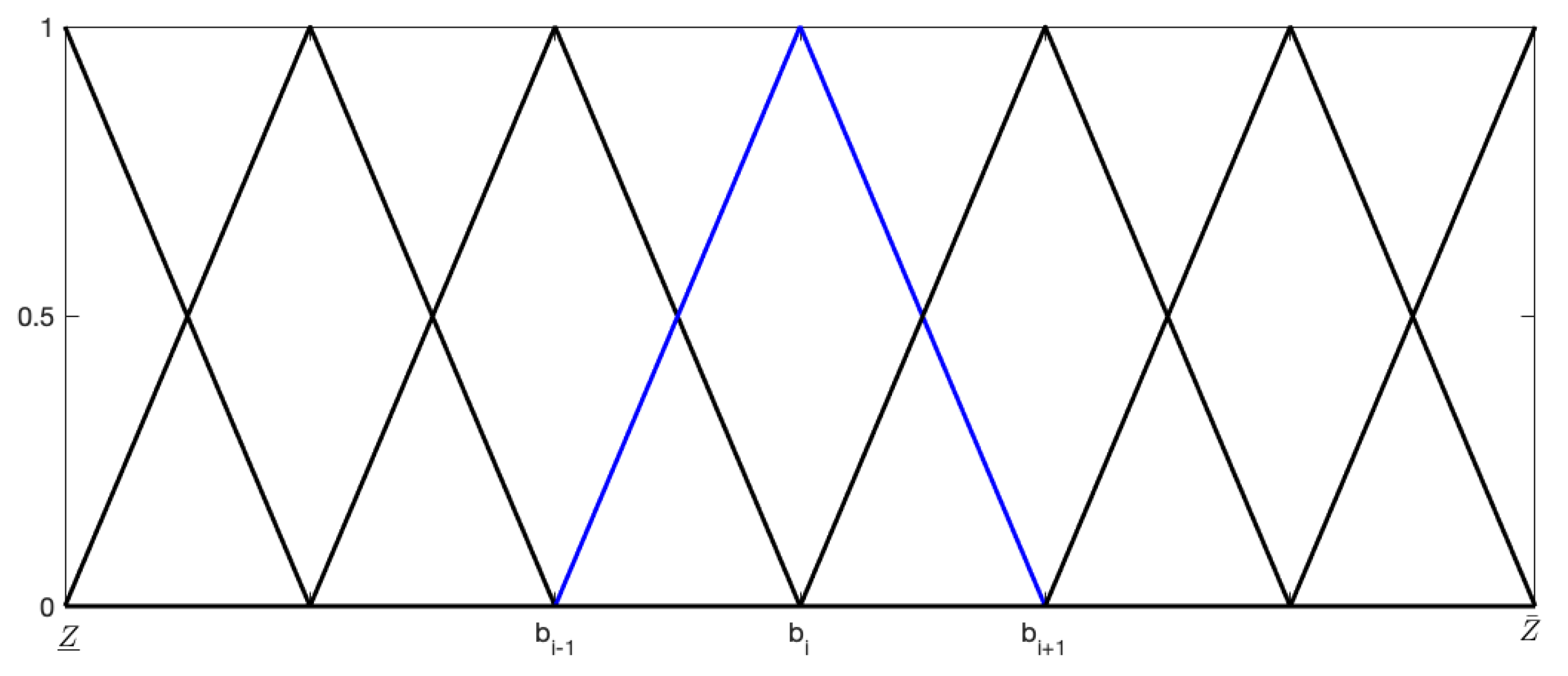
The proposed approach assumes that (4) can be divided into n sub-intervals, which are called degradation. Moreover, such classes can be uniformly spread out over the interval (4):
s i = z ̲ + ( i 1 ) z ¯ z ̲ n 1   i = 1 , , n .
Each of the above classes is associated with a triangular membership function shaped with [53]:
a i = b i 1 ,   b i = s i ,   c i = b i + 1 ,   i = 2 , , n 1 ,
a 1 = b 1 ,   c n = b n ,
where a i , b i , c i are the parameters that define the properties of the ith function (cf. Figure 7).
Representation of the system degradation with the use of membership functions allows to model this process in a T-S [19] form with the class model given by:
IF z k M z , i THEN z k = r k T p i + v k ,   i = 1 , , n ,
where M z , i is the fuzzy set associated with the ith membership function (6) and v k describes the uncertainty arising from measurement and modeling inaccuracies.
It should be noted that the fuzzy sets shaping (7) cover a feasible degradation spectrum from healthy ( z ̲ ) up to damaged ( z ¯ ). Thus, the degradation classes shaped by membership functions portrayed in Figure 7 can be easily explained and interpreted by humans. Additionally, from Figure 7, it can be seen that for any z ̲ z z ¯ , at most two IF–THEN rules are applied. Taking into consideration the fact that each IF–THEN rule is associated with the exponential model (3), the output of the proposed T-S framework is a fusion of two exponential models (3). As a result, a clear physical explanation of the T-S output can be stated in the sense of the system health assessment and prediction. The T-S representation of the considered system (7) can be redefined to the following form:
z k = i = 1 n μ i ( z k ) ( r k T p i + v k ) ,   with   i = 1 n μ i ( z k ) = 1 ,   and   μ i ( z k ) 0 ,
where μ i ( z k ) for i = 1 , , n denotes the normalized ith rule firing strength obtained on the basis of the triangular shape (6) and p i represents a parameters that should be estimated. To enable parameter estimation the system given by (8) has to be rewritten as:
z k = r ¯ k T p ¯ + v k ,
where r ¯ = [ μ 1 ( z k ) r k T , μ 2 ( z k ) r k T , , μ n ( z k ) r k T ] T denotes the regressor and p ¯ = [ ( p 1 ) T , , ( p n ) T ] T is the parameters vector.
An analysis of relation (9) shows that values of the system degradation z k depend on 2 n parameters included in p ¯ R 2 n . It should be underlined that for numerous practical applications the number of degradation classes n is rather small. Moreover, several of μ l ( z k ) correlated with a given class are inactive until the degradation process intensifies. In such cases some elements of the regressor vector are equal to zero, which significantly complicates the estimation process. This is the reason why triangular membership functions are employed. From Figure 7, it can be seen that for any x k only two membership functions are active. In such a case the relation (8) can be rewritten as:
z k = μ i ( z k ) r k T p i + μ i + 1 ( z k ) r k T p i + 1 + v k ,   μ i ( z k ) + μ i + 1 ( z k ) = 1 ,   μ i ( z k ) 0 ,
for i = 1 , , n 1 . In this way, a partial answer to Q2 is provided. Thus, while a new data sample is arriving, neighboring models are selected (see (10)), which in total contain four parameters only. This enables fast and reliable parameter estimation. Moreover, the entire approach was developed in such a way that at any time a new historical model can be introduced, and hence, the quality of the entire framework improves over the time history.
Another important factor affecting the process of parameter estimation is the assumption related to the character of the disturbances and modeling uncertainty represented by the vector v k . In numerous articles the knowledge of the statistical nature of these disturbances is assumed, e.g., normal distribution or the expected value is equal to zero [54]. Unlike the methods used so far in this article, it is proposed to assume that the values of v k are bounded by a known upper bound of v ¯ :
| v k | v ¯ .
In such a way the first part of Q1 is answered. Indeed, in such a case the value of v ¯ is perceived as a maximum difference between (10) and z m , k :
| z k z m , k | v ¯ ,
where z m , k is the output of the degradation model:
z m , k = μ i ( z k ) r k T p l i + μ i + 1 ( z k ) r k T p l i + 1 , μ i ( z k ) + μ i + 1 ( z k ) = 1 ,   μ i ( z k ) 0 ,   i = 1 , , n 1 .
The primary advantage of the proposed framework boils down to storing the parameter vector p ¯ l = [ ( p l 1 ) T , , ( p l n ) T ] T opposite to a possibly big dataset representing the information about degradation. This also signifies an answer to the first part of Q3.
In order to achieve p ¯ l , various recursive parameter estimation algorithms can be used [55]. One of them, which belongs to the class of so-called bounded error approaches [56,57], is the Quasi-Outer Bounding Ellipsoid algorithm (QOBE) [56]. This algorithm is characterized by a simplicity and performance comparable to the Recursive Least-Square (RLS) [58] one. It recommends its application to the on-line updating of degradation model parameters. Thus, by adapting the QOBE algorithm, the estimation of (13) is realized by the following algorithm:
Step 0: 
Assume the initial parameters: k = 1 , p 0 j = 0 for j = 1 , , n , moreover P 0 i = ρ I for i = 1 , , n 1 , wherein ρ > 0 .
Step 1: 
Obtain a set of active sub-models:
i = { j : μ j ( z k ) + μ j + 1 ( z k ) = 1 ,   for   j = 1 , , n 1 } .
Step 2: 
Assume:
r k i = [ μ i ( z k ) r k T , μ i + 1 ( z k ) r k T ] T ,   w k i = [ ( p k i ) T , ( p k i + 1 ) T ] T .
Step 3: 
Obtain:
e k i = z k ( r k i ) T w k 1 i .
Step 4: 
If | e k i | > v ¯ , then calculate:
g k i = ( r k i ) T P k i r k i ,
λ k i = g k i | e k i | v ¯ 1 ,
P k i = ( λ k i ) 1 ( P k 1 i P k 1 i r k i ( r k i ) T P k 1 i ( g k i ) 1 ) ,
w k i = w k 1 i + P k i r k i e k i ,
else:
P k i = P k 1 i ,
w k i = w k 1 i .
Step 5: 
Set k = k + 1 and go to Step 1.
The above five-step algorithm can be used for designing a set of T-S models corresponding to run-to-failure historical data of n h MOSFETs. The algorithm also completes the answer to question Q1 pertaining to preserving historical data in a possibly compact way.
Based on the algorithm for designing T-S historical models, an on-line algorithm for determining exponential model (3) can be easily derived. Indeed, it can be realized by removing Step 1 and Step 2 from the above five-step algorithm, which results in:
Step 0: 
Assume the initial parameters: k = 1 , p 0 = 0 , P 0 = ρ I , and ρ > 0 .
Step 1: 
Obtain:
e k = z k ( r k ) T w k 1 .
Step 2: 
If | e k | > v ¯ then calculate:
g k = ( r k ) T P k r k ,
λ k = g k | e k | v ¯ 1 ,
P k = ( λ k ) 1 ( P k 1 P k 1 r k ( r k ) T P k 1 ( g k ) 1 ) ,
w k = w k 1 + P k r k e k ,
else:
P k = P k 1 ,
w k = w k 1 .
Step 3: 
Set k = k + 1 and go to Step 1.
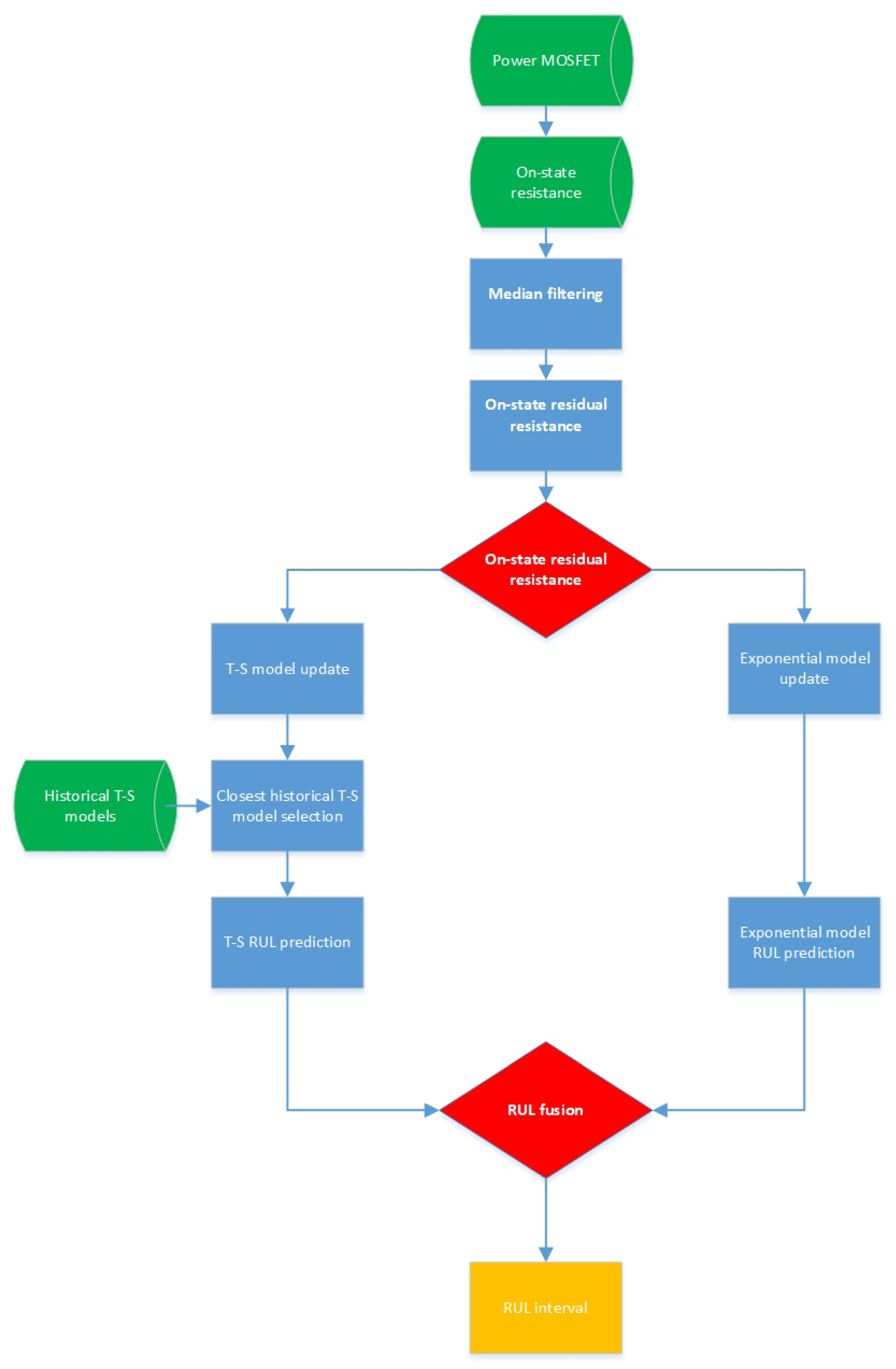
Having the above-proposed five-step and three-step algorithms, it is possible to propose an entire RUL estimation framework, which is presented in Figure 8.
Let us start with pointing out the fact that n h historical T-S models are stored in the Historical T-S models repository. It starts with selecting a currently operating Power MOSFET for RUL analysis. The next step is reduced to ON-state resistance R O N determination, which undergoes Median filtering. The subsequent point boils down to calculating the degradation signal z k , which is defined as On-state residual resistance. The values of z k = Δ R O N , k are determined as follows:
Δ R O N , k = R N O N R O N , k ,
where R N O N is a nominal on-state resistance R O N whilst R O N , k stands for one of the currently operating MOSFETs. Similarly, a percent change counterpart of (30) can be easily defined as:
δ R k = Δ R O N , k R N O N × 100 [ % ] .
After this important step, the degradation signal z k is fed to T-S model update and Exponential model update.
These two update mechanisms perform according to the five-step and three-steps algorithms, respectively, and they result in two different degradation models of the currently operating MOSFET. The objective of further deliberations is to:
  • Perform Closest historical T-S model selection.
  • Introduce the run-to-failure-based Historical T-S models repository for obtaining the RUL of a currently operating MOSFET.
  • Use an exponential model (3) for obtaining an alternative RUL prediction.
  • Perform an RUL fusion resulting in an RUL interval.
The realization of the above tasks constitutes final answers to questions Q2 and Q3.
As can be observed in Figure 8, after each iteration of the T-S model update the closest historical T-S model is selected for prediction purposes. This task is formally described by the optimization problem:
l = arg min l = 1 , , n h Q l i ,   Q l i = ( μ i ( z k ) r k T ( p l i p i ) + μ i + 1 ( z k ) r k T ( p l i + 1 p i + 1 ) ) 2 .
Having the lth T-S model, which is the closest one in the sense of (31), the prediction of the TTF t T S , f is performed:
f T S = z ¯ p 1 , l n T s p 2 , l n ,   t T S , f = T s × f T S .
where n signifies the sub-model of the lth model for which the failure threshold z ¯ was attained. Finally, the T-S-based RUL is calculated:
R U L T S , k = ( f T S k ) T s .
Similarly, after each iteration of the exponential model (3) update, the TTF and RUL are calculated as follows:
f E = z ¯ p 1 T s p 2 , l ,   t E , f = T s × f E ,
R U L E , k = ( f E k ) T s .
Finally, according to Figure 8, both RULs are fused to obtain a RUL interval, which is given by:
R U L k = [ min ( R U L E , k , R U L T S , k ) , max ( R U L E , k , R U L T S , k ) ] .
Having a complete RUL estimation framework, the objective of the next section is to perform a comprehensive experimental validation of the proposed approach.
As a final remark, it should be stated that the proposed RUL fusion always generates a feasible RUL interval. The worst cases of this interval are generated by either exponential or historical T-S models. Note that the former one can efficiently model a general degradation trend while the latter one makes it possible to incorporate a specific component behavior. Indeed, such behaviors are accumulated within the historical model database, which exhibits particular use cases. Thus, even though using historical T-S models some RUL fluctuations can be expected, they are fully justified by the same fluctuating behaviors in the past. Finally, it should be pointed out that the final decision is undertaken based on the RUL interval, which covers all above-mentioned behaviors.

4. Validation of the RUL Prediction Framework

4.1. Power MOSFETs Data Processing

As was already mentioned, datasets from the NASA Ames Prognostics Data Repository [23] were used for the validation purposes. In particular, the data containing measurements of the 42 power MOSFETs under thermal stress accelerated aging provided in [59] were applied during the experiments. The detailed description of the IRF520NPbF in a TO-220AB package is given in [60]. The IRF520NPbF MOSFETs were designated using HEXFET technology, i.e., the hexagonal structure, where a silicon oxide layer between the gate and source regions can be punctured by exceeding its dielectric strength. The considered MOSFETs use advanced processing techniques to obtain a very low on-resistance per silicon area. They can operate in a wide temperature range from −55 to +175 °C. These features combined with the fast switching speed make this system a very efficient and useful one in a wide variety of applications. It should be underlined that the IRF520NPbF MOSFETs are voltage-controlled elements and they can be connected directly to high-resistance sources. Therefore, they are suitable for use as switches and analog amplifiers. The MOSFETs being used are characterized by the following parameters:
  • Drain-to-source leakage current of −25 A;
  • Maximum continuous drain voltage of −100 V;
  • Continuous drain current of −9.7 A;
  • Minimum gate threshold voltage of −2 V;
  • Maximum gate threshold voltage of −4 V;
  • Internal drain inductance of −4.5 nH;
  • Internal source inductance of −7.5 nH.
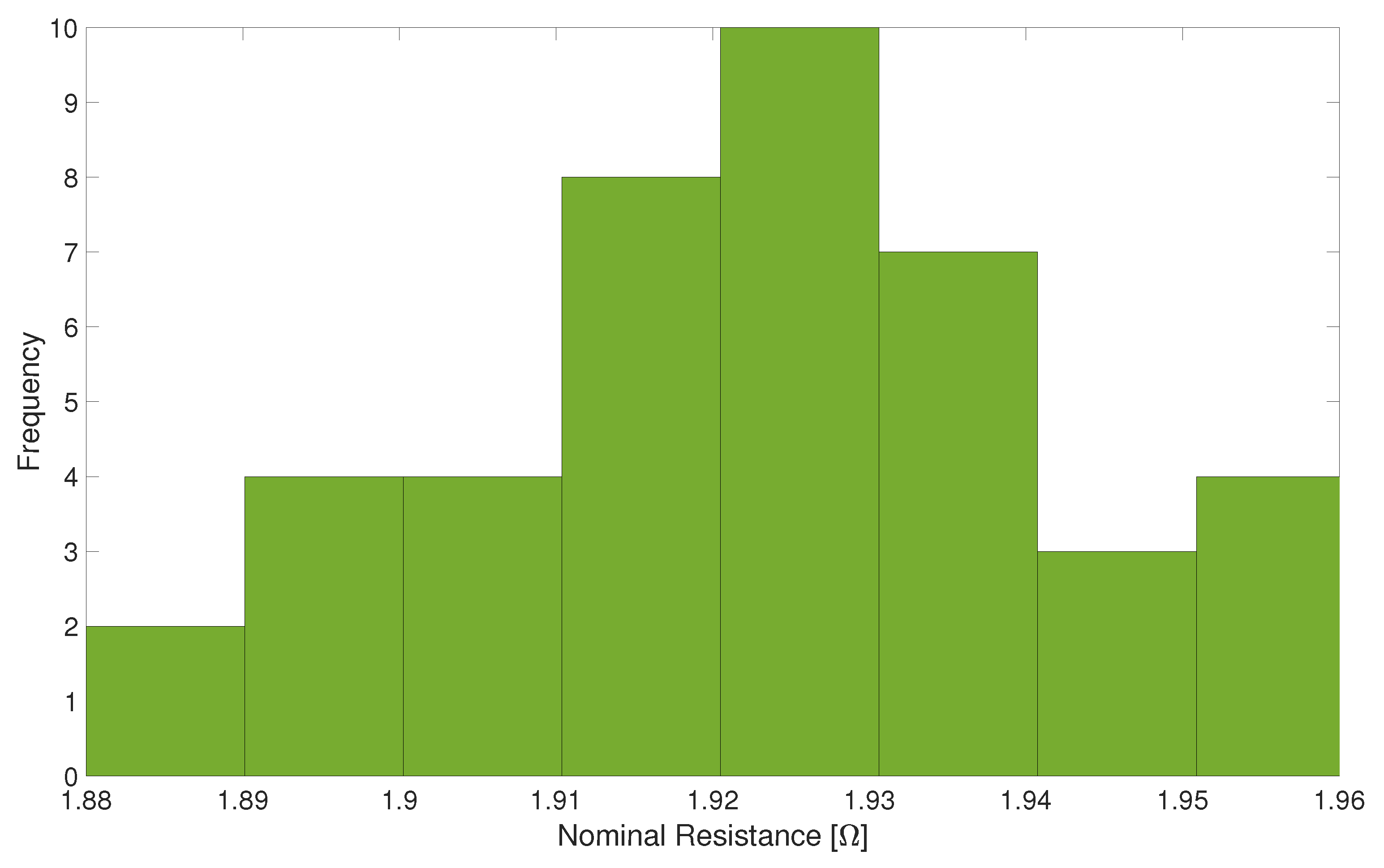
All tested transistors had the same ratings and type; however, they differed in the sense of their actual run-to-failure behavior. In spite of having the same type, they differed in the sense of their initial resistance. The histogram showing their resistance distribution is shown in Figure 9.
Concerning the aging process, following [59], the thermal cycling process was realized by feeding MOSFETs with suitable power cycles, and hence no external heat devices were employed. Moreover, the MOSFET temperature was measured and then directly employed as a control input for the application performing thermal cycling. To perform power cycling, the applied gate voltage had a form of a square wave characterized by a 15 V amplitude, 1 KHz frequency and a duty cycle of 40%. Moreover, the drain source was biased with 4 V DC while applying an additional load of 0.2 Ohm to the collector gate. Finally, the entire aging methodology is described in detail in [61]. Although the proposed approach is to be validated on the above MOSFET database, it can be used for any kind of electrical components in which either exponential or fluctuating RUL behavior can be expected. This, however, requires collecting a dataset such as the one described in [59].
Note that only values of drain source voltage V D S and drain current I D during the on-state gate were considered. Figure 10 shows exemplary data gathered from the 26th MOSFET. The drain current value decreases over time and the value of the drain source voltage increases.
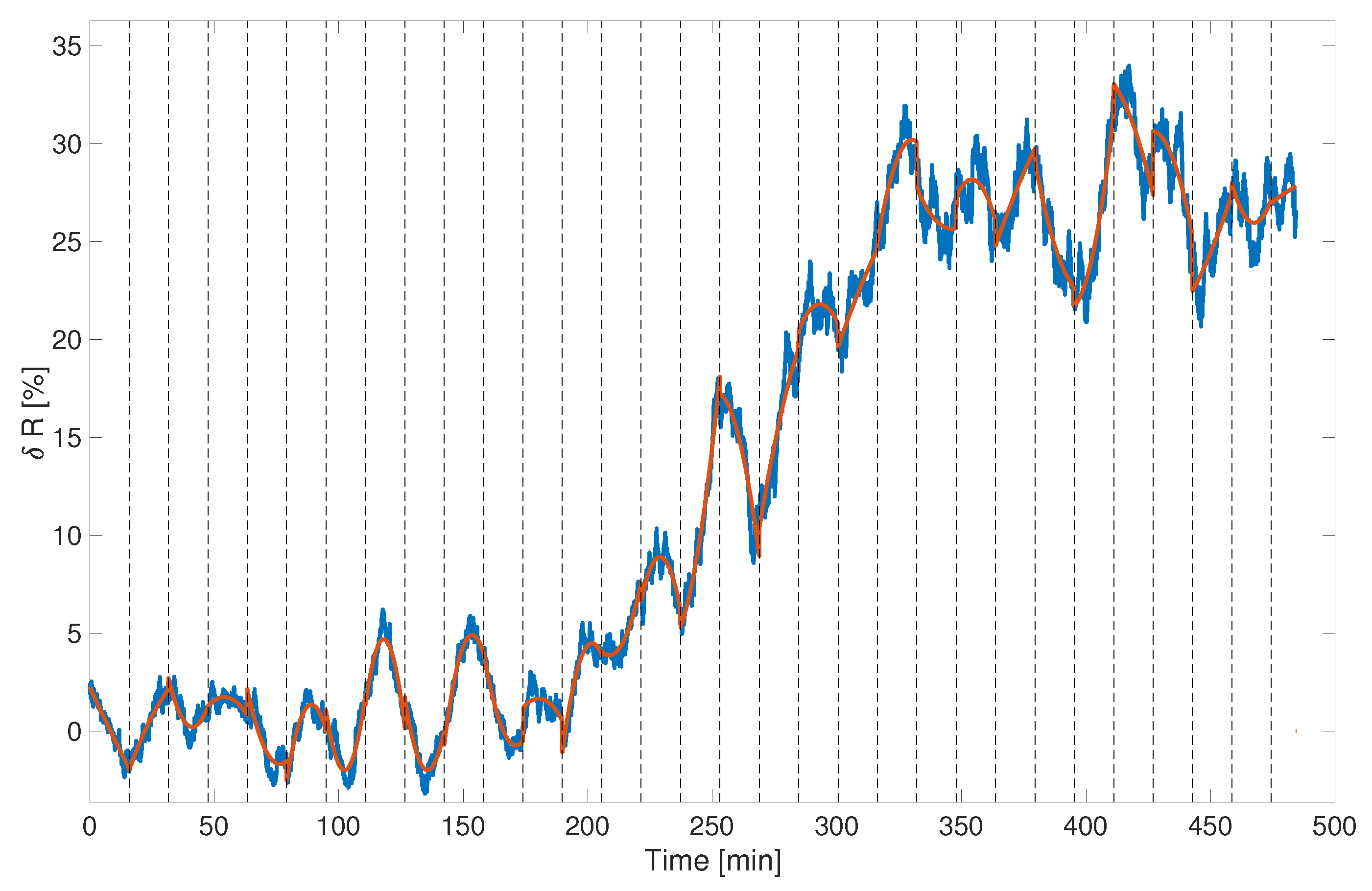
Using I D and V S D it is possible to compute the on-state resistance R O N of the MOSFETs. As depicted in Figure 8, the on-state resistance R O N was filtered using a median filter. Finally, Figure 11 presents filtered and unfiltered residual on-state resistance, which pertains to the 26th MOSFET. Let us remind the reader that this residual resistance is the degradation signal z k , which is used in the subsequent part of this paper.
The filtering process should be realized for all MOSFETs. However, for illustration purposes the degradation signals for six selected MOSFETs are presented in Figure 12. It should be noted that MOSFETs 6, 13 and 23 did not exhibit an exponential behavior. Thus, in this case, the standard exponential model should not be a judicious choice. Contrarily, the T-S model is capable of handling such a behavior. Thus, if the prospective MOSFET exhibits a similar behavior then it is expected that the proposed framework will respond in a desired way.

4.2. Design of Historical Model Repository

The determination of historical models was carried out in accordance with the methodology presented in Section 3.1. For that purpose, the following parameters were selected: T s = 0.85 s , z ̲ = 0.01 , z ¯ = 0.65 , n = 100 , v ¯ = 0.1 , ρ = 1 e 4 , n h = 20 and n = 10 . This means that 20 MOSFET models (No. 1, 2, 5, 6, 8, 10, 11, 13, 14, 15, 16, 21, 24, 25, 26, 29, 32, 33, 38 and 40) were selected for the historical repository whilst the degradation process was divided into 10 classes. Moreover, the same parameters are used in the remaining part of the paper. Figure 13 shows an exemplary result of the modeling process pertaining to the 13th MOSFET.
The number of classes can be, of course, extended depending on the degradation variability. Indeed, Figure 14 presents the T-S model for the 25th MOSFET, which contains 31 sub-models.

4.3. RUL Estimation and Prediction

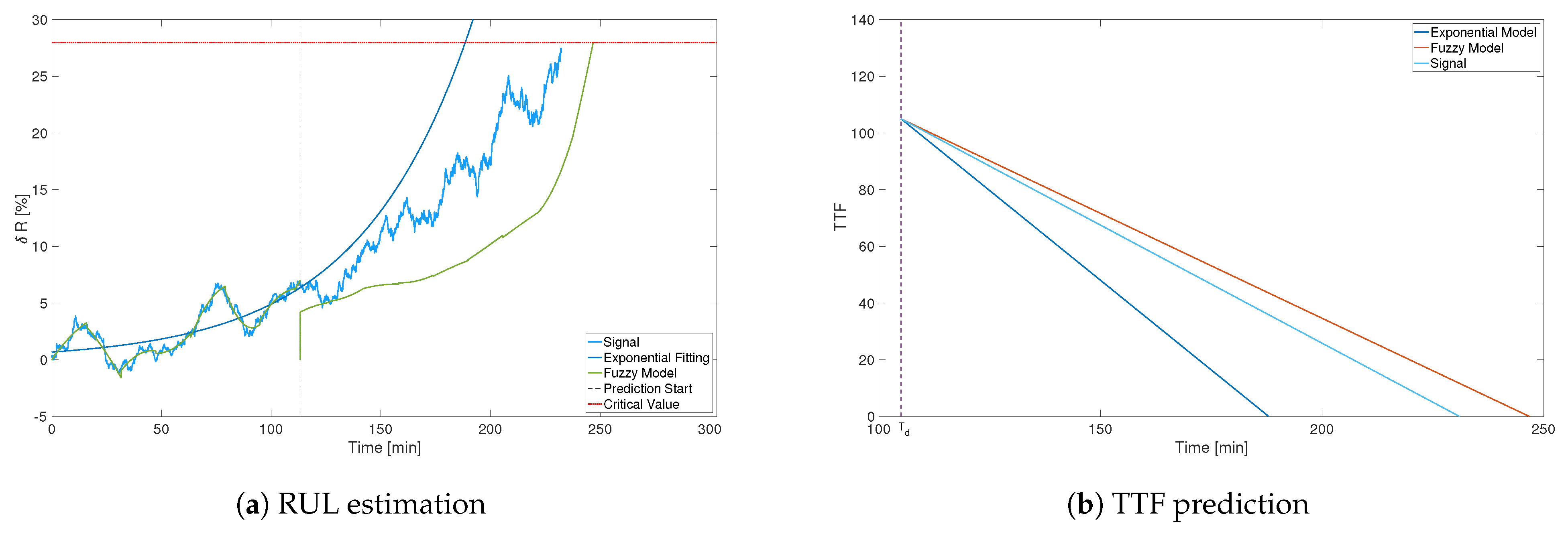
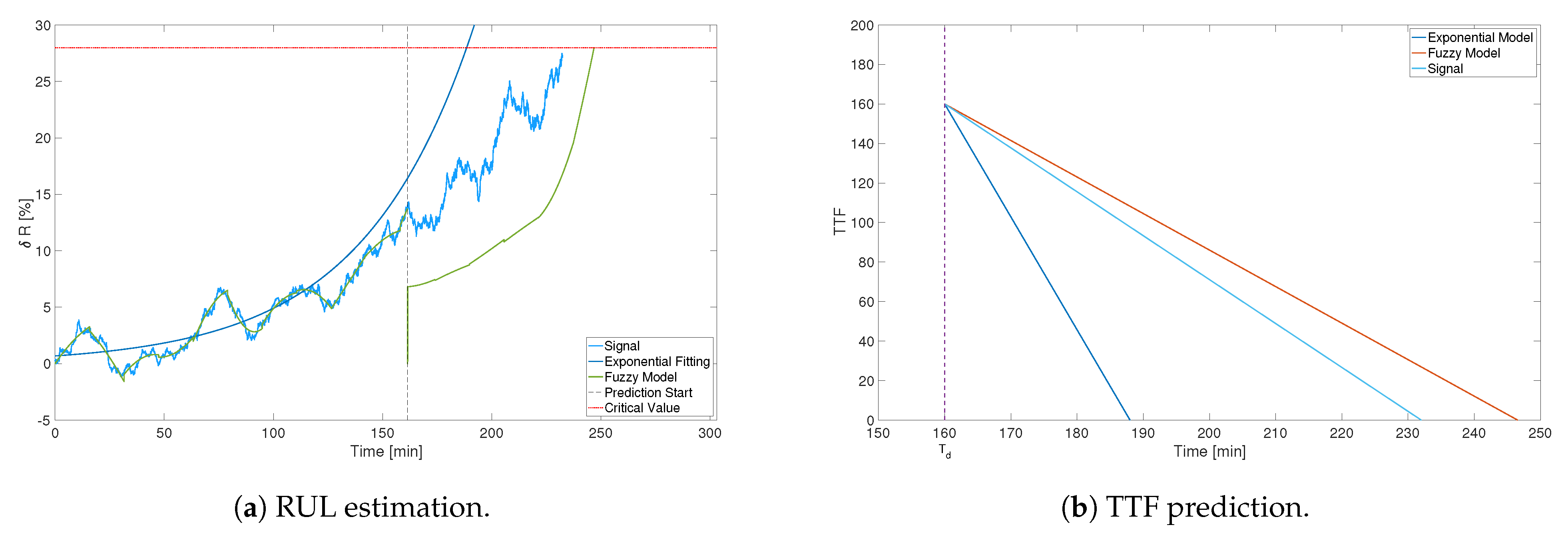
On the basis of the gathered historical models, the RUL prediction algorithm proposed in the preceding section was examined with the application of the MOSFETs not included in a historical model repository of n h = 20 transistors. Figure 15a shows RUL estimation results for the 36th MOSFET after 35 % of its real life time. According to (31), the proposed algorithm selected a historical model, which was the closest to the one currently operating. In parallel, the parameters of the exponential model were calculated and it was also used for prediction purposes. The resulting RUL and TTF prediction process is presented in Figure 15a,b.
Note that the TTF for the exponential model was equal to 280 min while for the T-S-based one is was 200 min. As a result, they form a suitable TTF interval, which can also be observed in the case of RUL.
A similar analysis was performed after 55 % of the entire MOSFET lifetime. The results are presented in Figure 16a. In this case, the estimation error provided by the T-S model was around 7 % . However, for the purposed decision the entire RUL interval should be taken into account.
The subsequent experiment pertains to the 23rd MOSFET, whose degradation signal did not exhibit an exponential nature. This MOSFET was intentionally selected to expose a behavior that is usually avoided in the approaches presented in the literature. Figure 17a presents the result of RUL and TTF analysis after 105 min (45%) of its entire lifetime. In this case, the exponential model definitely provided more pessimistic results than the ones obtained with the T-S framework.
Similar behavior can be observed after 65% of the entire lifetime. The obtained results are shown in Figure 18a. Again, the T-S model exhibited an error at the level of 6%. However, the entire RUL interval has to be taken into account while performing a final decision.
To make a fair performance assessment of the proposed approach, a comparative study with alternative solutions proposed in [59] was carefully performed. An alternative list of approaches operating on the same dataset were composed of:
  • Gaussian process regression;
  • Extended Kalman filter;
  • Particle filter.
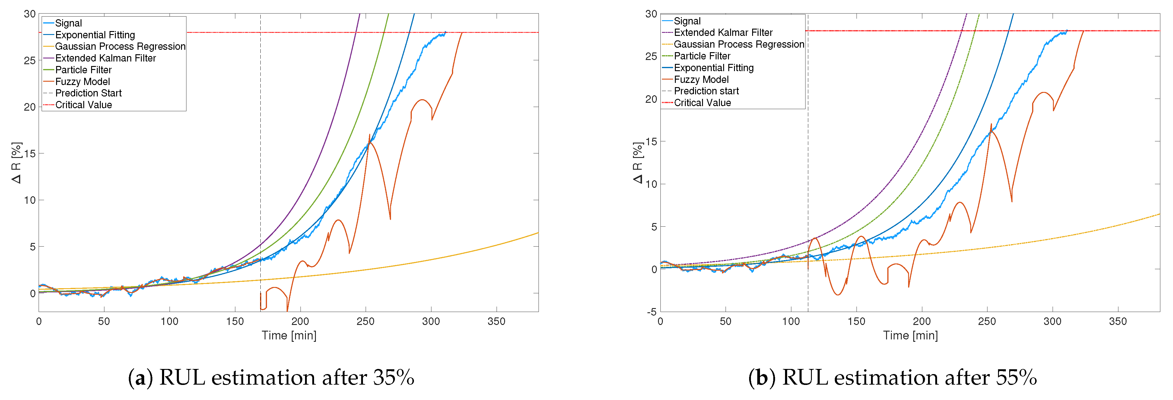
The obtained comparative study results for 35% of the entire lifetime are presented in Figure 19a. From these results, it is evident that proposed approach is superior over the others. The extended Kalman filter as the well as the particle filter behaved similarly to the proposed exponential models. This is caused by the fact that they have similar modeling roots. As expected, the particle filter dealt with nonlinearities in a more reliable way, and hence, its behavior was close to that of the exponential model.
Another comparison was realized after 55% of life (Figure 19b). As this is closer to the end of the entire lifetime, all methods provided better results. Thus, behavior is fully natural the closer the failure, and the easier it is to predict it. Nevertheless, the proposed approach still exhibited its superiority over the ones employed in [59]. Moreover, it should be pointed out that a comparison after 75% was also performed. The answers of alternative approaches were closer to the ones proposed in this paper. However, the general tendency was the same, and hence the presentation of these results was omitted.
In spite of the unquestionable appeal of the alternative approaches, they provide a point estimate of RUL without taking any historical MOSFET behavior into account. Contrarily, the proposed approach is based on a fusion of exponential and T-S actual/historical models resulting in an interval estimate of RUL. Such an interval is easier and more reliable at the level of final reasoning about MOSFET health.

5. Conclusions

In this paper, a novel joint analytical and data-driven health prognostic framework based on fuzzy logic was developed. The proposed approach is empolyed to enable the estimation and prediction of the RUL of any technical system. The idea behind the developed method is to use the Takagi–Sugeno multiple models-based framework for modeling of system degradation processes and RUL prediction. Unlike the conventional methods, the proposed approach designed on the basis of the analytical model and historical data forms an uncertainty interval containing an expected remaining useful life. Such a strategy enables effective support of diagnostic decisions in numerous practical cases. The proposed approach was validated using real data for power MOSFETs obtained from the NASA Ames Prognostics Data Repository. In the proposed method the status of the currently operating MOSFET was determined taking into consideration the knowledge obtained from the preceding MOSFETs, which went through the run-to-failure process. The performed MOSFET RUL prediction process enables the determination of the so-called time-to-failure along with its uncertainty interval, which enables earlier replacement of the diagnosed component before the failure of the entire system occurs. The developed approach is characterized by a low computational burden, which is very important during monitoring the health of systems in real time. Finally, this approach can be recommended to apply in diagnostic systems as a health-aware control system.
Apart from the above-listed features, the proposed approach has several prospective applications with a high practical importance. Indeed, the health of each asset containing MOSFETs can be individually assessed. Thus, having a fleet of such assets, e.g., a wind farm, it is possible to distribute the workload between them, which will maximize the worst RUL of the fleet. The same RUL-based strategy can be used for scheduling maintenance within the fleet as well as the optimization of preordering and procurement of spare parts.
Finally, it should be noted that the results presented in this paper are based on an accelerated aging dataset. This approach enables faster verification of the proposed RUL estimation and prediction methods. Basically, there is no difference between data coming from real systems and systems with accelerated aging. The behavior of the considered MOSFETs is the same in the both cases, as was presented in several papers [62,63,64] and references therein. The obtained results clearly indicate and recommend the application of the obtained approach to MOSFETs operating under normal operation conditions. The results presented in this paper are solely based on the NASA dataset pertaining to a fixed temperature of operating transistors. Indeed, the obtained results clearly indicate that the proposed approach provides good estimates of transistors’ remaining useful life. This raises the need for subsequent experiments under various working temperature scenarios. Thus, the objective of future developments is to design a benchmark circuit capable of handling such requirements. This will allow to compare the failure activation energy found between state-of-the-art models and the proposed one.

Author Contributions

M.W. developed the general RUL estimation strategy. M.M. proposed the structure of the RUL algorithms and prepared a state-of-the-art review. B.L. implemented the algorithms and applied them to the benchmark data set. He also performed a comprehensive algorithm performance analysis. All authors have read and agreed to the published version of the manuscript.

Funding

The work was supported by the National Science Centre of Poland under Grant: UMO-2017/27/B/ST7/00620.

Institutional Review Board Statement

None.

Informed Consent Statement

None.

Data Availability Statement

None.

Conflicts of Interest

The authors declare no conflict of interest.

Abbreviations

The following abbreviations are used in this manuscript:
ARMAAutoregressive-Moving Average Model
ANNArtificial Neural Network
EoLEnd of Life
FPTFirst Prediction Time
MOSFETMetal-Oxide Semiconductor Field-Effect Transistor
R O N On-State Resistance
RLSRecursive Least-Square
RULRemaining Useful Life
PHMPrognostics and Health Management
TTFTime-To-Failure
T-STakagi–Sugeno model
QOBEQuasi-Outer Bounding Ellipsoid algorithm

References

  1. Wu, Y.; Yin, S.; Li, H.; Dong, M. Modeling and Experimental Investigation of Electromagnetic Interference (EMI) for SiC-Based Motor Drive. Energies 2020, 13, 5173. [Google Scholar] [CrossRef]
  2. Cha, K.H.; Ju, C.T.; Kim, R.Y. Analysis and Evaluation of WBG Power Device in High Frequency Induction Heating Application. Energies 2020, 13, 5351. [Google Scholar] [CrossRef]
  3. Okilly, A.; Kim, N.; Baek, J. Inrush Current Control of High Power Density DC–DC Converter. Energies 2020, 13, 4301. [Google Scholar] [CrossRef]
  4. Li, H.; Liao, X.; Hu, Y.; Huang, Z.; Wang, K. Analysis of voltage variation in silicon carbide MOSFETs during turn-on and turn-off. Energies 2017, 10, 1456. [Google Scholar] [CrossRef] [Green Version]
  5. Zuev, A.; Zhirabok, A.; Filaretov, V. Fault identification in underwater vehicle thrusters via sliding mode observers. Int. J. Appl. Math. Comput. Sci. 2020, 30. [Google Scholar] [CrossRef]
  6. Zhou, D.; Ji, H.; He, X.; Shang, J. Fault detection and isolation of the brake cylinder system for electric multiple units. IEEE Trans. Control Syst. Technol. 2017, 26, 1744–1757. [Google Scholar] [CrossRef]
  7. Zhang, H.; Tolbert, L. Efficiency impact of silicon carbide power electronics for modern wind turbine full scale frequency converter. IEEE Trans. Ind. Electron. 2010, 58, 21–28. [Google Scholar] [CrossRef]
  8. Simani, S.; Farsoni, S.; Castaldi, P. Data–Driven Techniques for the Fault Diagnosis of a Wind Turbine Benchmark. Int. J. Appl. Math. Comput. Sci. 2018, 28, 247–268. [Google Scholar] [CrossRef] [Green Version]
  9. Tsai, W.C. Optimization of Operating Parameters for Stable and High Operating Performance of a GDI Fuel Injector System. Energies 2020, 13, 2405. [Google Scholar] [CrossRef]
  10. Tsai, C.T.; Chen, W.M. Buck converter with soft-switching cells for PV panel applications. Energies 2016, 9, 148. [Google Scholar] [CrossRef] [Green Version]
  11. Pang, X.; Huang, R.; Wen, J.; Shi, Y.; Jia, J.; Zeng, J. A lithium-ion battery RUL prediction method considering the capacity regeneration phenomenon. Energies 2019, 12, 2247. [Google Scholar] [CrossRef] [Green Version]
  12. Salazar, J.C.; Sanjuan, A.; Nejjari, F.; Sarrate, R. Health–Aware and Fault–Tolerant Control of an Octorotor UAV System Based on Actuator Reliability. Int. J. Appl. Math. Comput. Sci. 2020, 30, 47–59. [Google Scholar]
  13. Do, N.V.; Nguyen, H.D.; Selamat, A. Knowledge-based model of expert systems using rela-model. Int. J. Softw. Eng. Knowl. Eng. 2018, 28, 1047–1090. [Google Scholar] [CrossRef]
  14. Chudnovsky, B.H. Electrical Equipment Life Expectancy, Aging, and Failures. In Electrical Power Transmission and Distribution; CRC Press: Boca Raton, FL, USA, 2017; pp. 269–308. [Google Scholar]
  15. Wang, C.; Lu, N.; Wang, S.; Cheng, Y.; Jiang, B. Dynamic long short-term memory neural-network-based indirect remaining-useful-life prognosis for satellite lithium-ion battery. Appl. Sci. 2018, 8, 2078. [Google Scholar] [CrossRef] [Green Version]
  16. Sun, B.; Li, Y.; Wang, Z.; Ren, Y.; Feng, Q.; Yang, D.; Lu, M.; Chen, X. Remaining useful life prediction of aviation circular electrical connectors using vibration-induced physical model and particle filtering method. Microelectron. Reliab. 2019, 92, 114–122. [Google Scholar] [CrossRef]
  17. Gebraeel, N.; Lawley, M.; Li, R.; Ryan, J. Residual-life distributions from component degradation signals: A Bayesian approach. IIE Trans. 2005, 37, 543–557. [Google Scholar] [CrossRef]
  18. Li, N.; Lei, Y.; Lin, J.; Ding, S. An improved exponential model for predicting remaining useful life of rolling element bearings. IEEE Trans. Ind. Electron. 2015, 62, 7762–7773. [Google Scholar] [CrossRef]
  19. Tanaka, K.; Sugeno, M. Stability analysis and design of fuzzy control systems. Fuzzy Sets Syst. 1992, 45, 135–156. [Google Scholar] [CrossRef]
  20. Witczak, M. Fault Diagnosis and Fault-Tolerant Control Strategies for Non-Linear Systems; Lectures Notes in Electrical Engineering; Springer International Publisher: Berlin/Heidelberg, Germany, 2014; Volume 266. [Google Scholar]
  21. Salcedo, J.V.; Martínez, M.; García-Nieto, S.; Hilario, A. T–S Fuzzy Bibo Stabilisation of Non–Linear Systems Under Persistent Perturbations Using Fuzzy Lyapunov Functions and Non–PDC Control Laws. Int. J. Appl. Math. Comput. Sci. 2020, 30, 529–550. [Google Scholar]
  22. Li, M.; Yu, D.; Chen, Z.; Xiahou, K.; Ji, T.; Wu, Q. A data-driven residual-based method for fault diagnosis and isolation in wind turbines. IEEE Trans. Sustain. Energy 2018, 10, 895–904. [Google Scholar] [CrossRef]
  23. Celaya, J.; Saxena, A.; Saha, S.; Goebel, K. MOSFET Thermal Overstress Aging Data Set. NASA AMES Prognostics Data Repository. 2007. Available online: https://ti.arc.nasa.gov/c/37/ (accessed on 10 April 2021).
  24. Wahle, P.; Schrimpf, R.; Galloway, K. Simulated space radiation effects on power MOSFETs in switching power supplies. IEEE Trans. Ind. Appl. 1990, 26, 798–802. [Google Scholar] [CrossRef]
  25. Dupont, L.; Lefebvre, S.; Bouaroudj, M.; Khatir, Z.; Faugières, J.C. Failure modes on low voltage power MOSFETs under high temperature application. Microelectron. Reliab. 2007, 47, 1767–1772. [Google Scholar] [CrossRef]
  26. Chen, Y.; Peng, G.; Zhu, Z.; Li, S. A novel deep learning method based on attention mechanism for bearing remaining useful life prediction. Appl. Soft Comput. 2020, 86, 105–919. [Google Scholar] [CrossRef]
  27. Li, X.; Ding, Q.; Sun, J.Q. Remaining useful life estimation in prognostics using deep convolution neural networks. Reliab. Eng. Syst. Saf. 2018, 172, 1–11. [Google Scholar] [CrossRef] [Green Version]
  28. Wagner, W.P. Trends in expert system development: A longitudinal content analysis of over thirty years of expert system case studies. Expert Syst. Appl. 2017, 76, 85–96. [Google Scholar] [CrossRef]
  29. Mrugalska, B. A bounded-error approach to actuator fault diagnosis and remaining useful life prognosis of Takagi–Sugeno fuzzy systems. ISA Trans. 2018, 80, 257–266. [Google Scholar] [CrossRef] [PubMed]
  30. Chu, A.; Allam, A.; Arenas, A.C.; Rizzoni, G.; Onori, S. Stochastic capacity loss and remaining useful life models for lithium-ion batteries in plug-in hybrid electric vehicles. J. Power Sources 2020, 478, 228991. [Google Scholar] [CrossRef]
  31. Ossai, C.I.; Raghavan, N. Statistical characterization of the state-of-health of lithium-ion batteries with Weibull distribution function—A consideration of random effect model in charge capacity decay estimation. Batteries 2017, 3, 32. [Google Scholar] [CrossRef] [Green Version]
  32. Wang, D.; Tsui, K.L. Statistical modeling of bearing degradation signals. IEEE Trans. Reliab. 2017, 66, 1331–1344. [Google Scholar] [CrossRef]
  33. Benker, M.; Furtner, L.; Semm, T.; Zaeh, M.F. Utilizing uncertainty information in remaining useful life estimation via Bayesian neural networks and Hamiltonian Monte Carlo. J. Manuf. Syst. 2020. [Google Scholar] [CrossRef]
  34. Li, W.; Liu, T. Time varying and condition adaptive hidden Markov model for tool wear state estimation and remaining useful life prediction in micro-milling. Mech. Syst. Signal Process. 2019, 131, 689–702. [Google Scholar] [CrossRef]
  35. Chen, Z.; Li, Y.; Xia, T.; Pan, E. Hidden Markov model with auto-correlated observations for remaining useful life prediction and optimal maintenance policy. Reliab. Eng. Syst. Saf. 2019, 184, 123–136. [Google Scholar] [CrossRef]
  36. Nielsen, J.S.; Sørensen, J.D. Bayesian estimation of remaining useful life for wind turbine blades. Energies 2017, 10, 664. [Google Scholar] [CrossRef] [Green Version]
  37. Mosallam, A.; Medjaher, K.; Zerhouni, N. Data-driven prognostic method based on Bayesian approaches for direct remaining useful life prediction. J. Intell. Manuf. 2016, 27, 1037–1048. [Google Scholar] [CrossRef]
  38. Baptista, M.; Henriques, E.M.; de Medeiros, I.P.; Malere, J.P.; Nascimento, C.L., Jr.; Prendinger, H. Remaining useful life estimation in aeronautics: Combining data-driven and Kalman filtering. Reliab. Eng. Syst. Saf. 2019, 184, 228–239. [Google Scholar] [CrossRef]
  39. Cui, L.; Wang, X.; Xu, Y.; Jiang, H.; Zhou, J. A novel switching unscented Kalman filter method for remaining useful life prediction of rolling bearing. Measurement 2019, 135, 678–684. [Google Scholar] [CrossRef]
  40. Sikorska, J.; Hodkiewicz, M.; Ma, L. Prognostic modeling options for remaining useful life estimation by industry. Mech. Syst. Signal Process. 2011, 25, 1803–1836. [Google Scholar] [CrossRef]
  41. Lei, Y.; Li, N.; Lin, J. A new method based on stochastic process models for machine remaining useful life prediction. IEEE Trans. Instrum. Meas. 2016, 65, 2671–2684. [Google Scholar] [CrossRef]
  42. Li, N.; Lei, Y.; Guo, L.; Yan, T.; Lin, J. Remaining useful life prediction based on a general expression of stochastic process models. IEEE Trans. Ind. Electron. 2017, 64, 5709–5718. [Google Scholar] [CrossRef]
  43. Baptista, M.; Sankararaman, S.; de Medeiros, I.P.; Nascimento, C., Jr.; Prendinger, H.; Henriques, E.M. Forecasting fault events for predictive maintenance using data-driven techniques and ARMA modeling. Comput. Ind. Eng. 2018, 115, 41–53. [Google Scholar] [CrossRef]
  44. Long, Y.; Luo, H.; Zhi, Y.; Wang, X. Remaining Useful Life Estimation of Solder joints using an ARMA Model Optimized by Genetic Algorithm. In Proceedings of the 2018 19th International Conference on Electronic Packaging Technology (ICEPT), Shanghai, China, 8–11 August 2018; pp. 1108–1111. [Google Scholar]
  45. Xia, M.; Li, T.; Liu, L.; Xu, L.; Gao, S.; De Silva, C.W. Remaining useful life prediction of rotating machinery using hierarchical deep neural network. In Proceedings of the 2017 IEEE International Conference on Systems, Man, and Cybernetics (SMC), Banff, AB, Canada, 5–8 October 2017; pp. 2778–2783. [Google Scholar]
  46. Mrugalski, M. Advanced Neural Network-Based Computational Schemes for Robust Fault Diagnosis; Springer International Publishing: Berlin/Heidelberg, Germany, 2014. [Google Scholar]
  47. Witczak, M.; Mrugalski, M.; Korbicz, J. Towards Robust Neural-Network-Based Sensor and Actuator Fault Diagnosis: Application to a Tunnel Furnace. Neural Process. Lett. 2015, 42, 71–87. [Google Scholar] [CrossRef] [Green Version]
  48. Wu, J.; Su, Y.; Cheng, Y.; Shao, X.; Deng, C.; Liu, C. Multi-sensor information fusion for remaining useful life prediction of machining tools by adaptive network based fuzzy inference system. Appl. Soft Comput. 2018, 68, 13–23. [Google Scholar] [CrossRef]
  49. Lei, Y.; Li, N.; Gontarz, S.; Lin, J.; Radkowski, S.; Dybala, J. A model-based method for remaining useful life prediction of machinery. IEEE Trans. Reliab. 2016, 65, 1314–1326. [Google Scholar] [CrossRef]
  50. Zhang, L.; Mu, Z.; Sun, C. Remaining useful life prediction for lithium-ion batteries based on exponential model and particle filter. IEEE Access 2018, 6, 17729–17740. [Google Scholar] [CrossRef]
  51. Anis, M.D. Towards Remaining Useful Life Prediction in Rotating Machine Fault Prognosis: An Exponential Degradation Model. In Proceedings of the 2018 Condition Monitoring and Diagnosis (CMD), Perth, Australia, 23–26 September 2018; pp. 1–6. [Google Scholar]
  52. Lu, C.J.; Meeker, W.O. Using degradation measures to estimate a time-to-failure distribution. Technometrics 1993, 35, 161–174. [Google Scholar] [CrossRef]
  53. Zadeh, L.A. Knowledge representation in fuzzy logic. In Fuzzy Sets, Fuzzy Logic, and Fuzzy Systems: Selected Papers by Lotfi a Zadeh; World Scientific: Singapore, 1996; pp. 764–774. [Google Scholar]
  54. Söderström, T.; Stoica, P. System Identification; Prentice-Hall International: Hoboken, NJ, USA, 1989. [Google Scholar]
  55. Cowan, C.F.; Grant, P.M. Adaptive Filters; Prentice-Hall: Englewood Cliffs, NJ, USA, 1985; Volume 152. [Google Scholar]
  56. Arablouei, R.; Doğançay, K. Modified quasi-OBE algorithm with improved numerical properties. Signal Process. 2013, 93, 797–803. [Google Scholar] [CrossRef]
  57. Kraus, T.; Mandour, G.I.; Joachim, D. Estimating the error bound in QOBE Vowel classification. In Proceedings of the 2007 50th Midwest Symposium on Circuits and Systems, Montreal, QC, Canada, 5–8 August 2007; pp. 369–372. [Google Scholar]
  58. Bottomley, G.; Alexander, S. A theoretical basis for divergence of conventional recursive least squares filters. In Proceedings of the International Conference on Acoustics, Speech, and Signal Processing, Glasgow, UK, 23–26 May 1989; pp. 908–911. [Google Scholar]
  59. Celaya, J.; Saxena, A.; Saha, S.; Goebel, K.F. Prognostics of power MOSFETs under thermal stress accelerated aging using data-driven and model-based methodologies. In Proceedings of the Annual Conference of the Prognostics and Health Management Society, Denver, CO, USA, 20–23 June 2011. [Google Scholar]
  60. Mosfet TO220AB Datasheet. Available online: http://pdf.datasheetcatalog.com/datasheets2/73/73619_1.pdf (accessed on 17 March 2021).
  61. Celaya, J.R.; Saxena, A.; Wysocki, P.; Saha, S.; Goebel, K. Towards Prognostics of Power MOSFETs: Accelerated Aging and Precursors of Failure; Technical Report; National Aeronautics and Space Administrations Moffett Field CA AMES Research: Mountain View, CA, USA, 2010.
  62. Patil, N.; Celaya, J.; Das, D.; Goebel, K.; Pecht, M. Precursor parameter identification for insulated gate bipolar transistor (IGBT) prognostics. IEEE Trans. Reliab. 2009, 58, 271–276. [Google Scholar] [CrossRef]
  63. Saha, S.; Celaya, J.R.; Vashchenko, V.; Mahiuddin, S.; Goebel, K.F. Accelerated aging with electrical overstress and prognostics for power MOSFETs. In Proceedings of the IEEE 2011 EnergyTech, Cleveland, OH, USA, 25–26 May 2011; pp. 1–6. [Google Scholar]
  64. Celaya, J.R.; Wysocki, P.; Vashchenko, V.; Saha, S.; Goebel, K. Accelerated aging system for prognostics of power semiconductor devices. In Proceedings of the 2010 IEEE Autotestcon, Orlando, FL, USA, 13–16 September 2010; pp. 1–6. [Google Scholar]
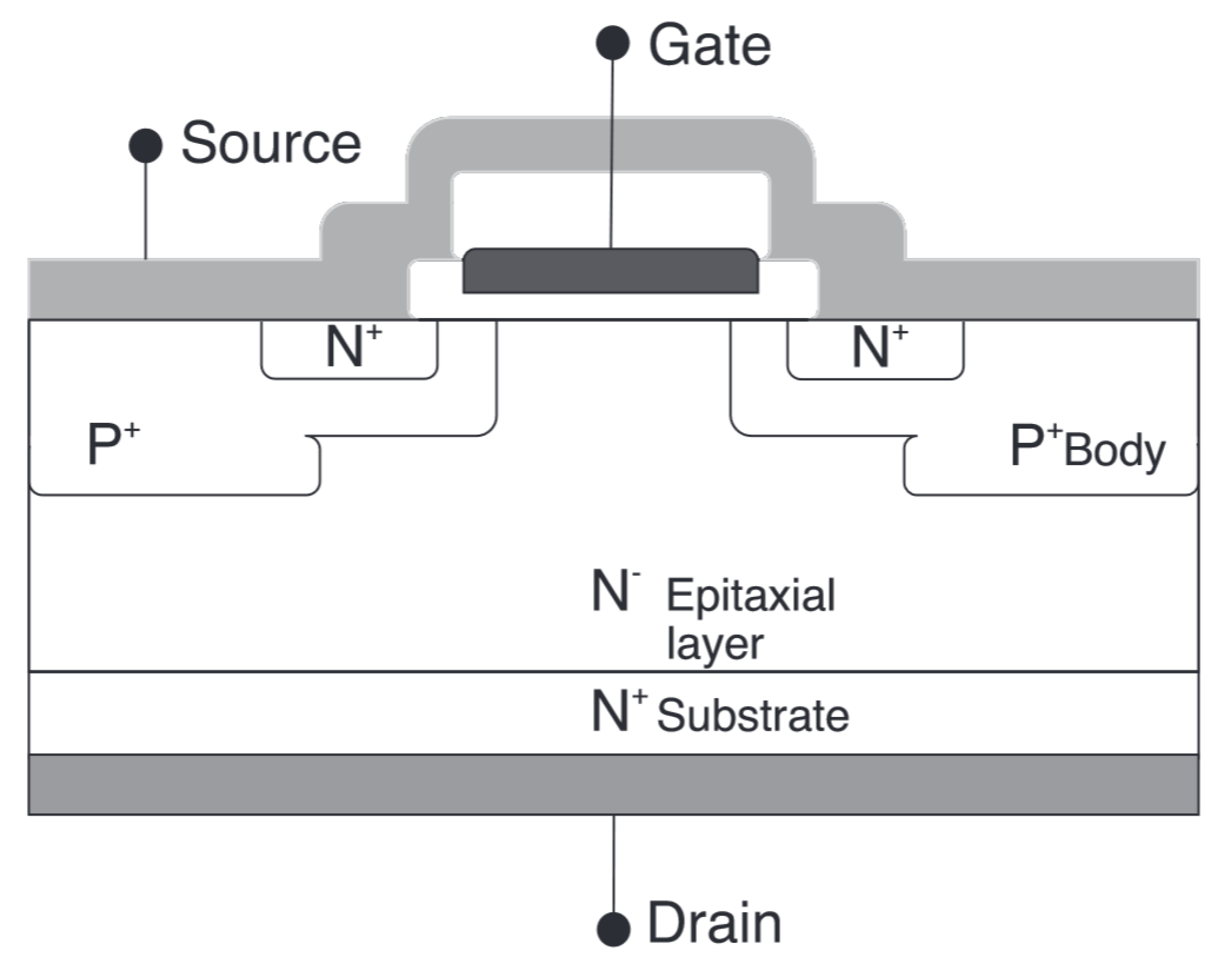
Figure 1. The structure of a power Metal Oxide Field Effect Transistors (MOSFETs).
Energies 14 02135 g001
Figure 2. Concept of Remaining Useful Life (RUL).
Energies 14 02135 g002
Figure 3. RUL prediction.
Energies 14 02135 g003
Figure 4. Methodology of RUL prediction with Takagi-Sugeno (T-S) degradation model.
Energies 14 02135 g004
Figure 5. Scheme of MOSFET aging system.
Energies 14 02135 g005
Figure 6. Thermal block and its application for MOSFETs’ accelerated aging.
Energies 14 02135 g006
Figure 7. MOSFET degradation classes shaped by membership functions.
Energies 14 02135 g007
Figure 8. Flowchart of the proposed framework.
Energies 14 02135 g008
Figure 9. Histogram of nominal resistance.
Energies 14 02135 g009
Figure 10. Current, voltage and resistance of the 26th MOSFET.
Energies 14 02135 g010
Figure 11. δ R and filtered δ R for MOSFET 26.
Energies 14 02135 g011
Figure 12. Exemplary filtered degradation signals for MOSFETs 6, 13, 23, 24, 26 and 36.
Energies 14 02135 g012
Figure 13. Exemplary learning results for the 13th MOSFET.
Energies 14 02135 g013
Figure 14. Exemplary learning results for the 25th MOSFET.
Energies 14 02135 g014
Figure 15. RUL and Time-To-Failure (TTF) analysis of the 36th MOSFET after 35% of its real lifetime.
Energies 14 02135 g015
Figure 16. RUL and TTF analysis of the 36th MOSFET after 55% of its real lifetime.
Energies 14 02135 g016
Figure 17. RUL and TTF analysis of the 23th MOSFET after 45% of its real lifetime.
Energies 14 02135 g017
Figure 18. RUL and TTF analysis of the 23th MOSFET after 65% of its real lifetime.
Energies 14 02135 g018
Figure 19. Comparison of RUL predictions by different methods.
Energies 14 02135 g019
Publisher’s Note: MDPI stays neutral with regard to jurisdictional claims in published maps and institutional affiliations.