
Sampling Primary Power Standard from DC up to 9 kHz Using Commercial Off-The-Shelf Components †


Laboratory Electrical Energy and Power, Federal Institute of Metrology METAS, 3003 Bern-Wabern, Switzerland
†
This paper is an extended version of our paper published in the proceedings of the Third International Colloquium on Intelligent Grid Metrology (Smagrimet 2020).
Energies 2021, 14(8), 2203; https://doi.org/10.3390/en14082203
Submission received: 2 March 2021
/
Revised: 1 April 2021
/
Accepted: 7 April 2021
/
Published: 15 April 2021
(This article belongs to the Special Issue Power System Simulation, Control and Optimization Ⅱ)
Abstract
:In the framework of the empir projects myrails and windefcy, metas developed a primary standard for electrical power using commercial off-the-shelf components. The only custom part is the software that controls the sampling system and determines the amplitude and phase of the different frequency components of voltage and current. The system operates from dc up to 9 kHz, even with distorted signals. The basic system is limited to 700 V and 21 A. Its power uncertainty is 15 μW/VA at power frequencies and increases to mW/VA at 9 kHz. With the extension up to 1000 V and 360 A, the system reaches power uncertainties of 20 μW/VA at power frequencies, increasing to 510 μW/VA at 9 kHz. For higher voltages or higher currents, the same principle is used. However, the uncertainties are dominated by the stability of the sources. The voltage and current channels can also be used independently to calibrate and test power quality instruments. Thanks to a time-stamping system, the system can also be used to calibrate phasor measurement units, which are synchronised to utc.
Keywords:
electrical power; EMPIR; MyRailS; WindEFCY; PMU; power quality; power standard; sampling; traceability; uncertainty
1. Introduction
In the framework of the empir project myrails [1], calibration facilities for energy meters and power quality monitoring systems were developed for railway applications. In the framework of the empir project windefcy [2], calibration facilities for synchronised electrical power measurement are developed as part of an efficiency measurement set-up for wind turbines.
As part of its contribution, metas, the Swiss national metrology institute, developed a primary standard for electrical power using a power calibrator as voltage and current source, shunts, sampling voltmeters and a time-stamping system (Section 2). All hardware is based on commercial off-the-shelf (cots) components to make the system easily reproducible and maintainable. Custom software controls the sampling system and determines the amplitude and phase of the different frequency components of voltage and current [3]. The system operates from dc up to 9 kHz, with both pure and distorted signals. The active power uncertainty is 15 μW/VA at power frequencies and increases to mW/VA at 9 kHz (Section 3).
Demonstrated metrological traceability is essential in science. Without it, scientific results cannot be compared [4]. Comparability is essential to reproducibility, and reproducibility is a fundamental principle of science [5]. In industrial applications, traceability is a requirement for quality, since, otherwise, the compliance with specifications cannot be shown. Consequently, traceability is a requirement of iso/iec 17025 [6]. Therefore, this system was used in a comparison (Section 4) with ptb, the German national metrology institute, with pure sine signals at 120 and 240 V, 5 A, and Hz. The active power measurements of the primary power standards of metas and ptb agree within 4 μW/VA.
With the extension (Section 5) up to 1000 V and 360 A, power uncertainties of 20 μW/VA are reached at power frequencies, increasing to 510 μW/VA at 9 kHz. For higher voltages or higher currents, the same principle is used. Currents of multiple kiloamperes and voltages in excess of 100 kV can be generated in transformer calibration labs such as metas’s. The corresponding sources can be integrated into this system provided they allow for synchronisation of the voltage and current channels. The uncertainties are usually dominated by the stability of the sources and need to be evaluated for every individual case.
The voltage and current channels of all proposed variants can also be used independently to calibrate power quality instruments [7,8,9]. A time-stamping system is used to synchronise the measurements to utc [10]. This is particularly useful in power quality and phasor measurement unit applications, where the duts are also synchronised to utc, since, in practical applications, their input signals vary rapidly or the phasors at different locations need to be compared. Therefore, such instruments need to time-stamp their measurements to make measurements from different instruments comparable.
The calibration facilities are used to provide traceability to metas’s meter testing and certification system. The latter is also used at dc, for railway applications [11,12] and for other applications for which a standard is currently in the last stages of development [13]. An application of quickly growing relevance is electric vehicle charging. To develop the metrology framework for dc electricity grids, the proposal 20nrm03 dc grids has been submitted in response to [14].
2. Measurement Set-Up and Characterisation
The basic set-up (Figure 1) is composed of calibrated reference instruments providing traceability to the si, a source providing the required voltages and currents, as well as the dut. The dut is provided by the customer and changes frequently. It is part of the set-up, but not of the reference system, which consists of the following components.
- One three-phase power calibrator Fluke 6105A/6135A or similar. In this set-up, the essential property is the stability of the outputs and the operating range ( A, kHz).
- Three calibrated shunts Fluke A40B or similar.
- Six calibrated sampling voltmeters Keysight 3458A or similar with a trigger input and aperture waveform output. The 3458A is well documented (e.g., [15]). It limits the maximum voltage to V.
- One utc-synchronised six-channel time-to-digital converter (tdc), e.g., three ni pxi-6683.
The system is easily scalable. It can be set up for any number of phases.
This system was presented at Smargimet 2020 [16]. For currents A and voltages V, the system has since been extended.
2.1. Characterisation of the Shunts
Shunts are used to convert currents into voltages, which are sampled by the voltmeters. The power calculation is directly affected by the properties of the shunts. For the determination of power, the phase difference between voltage and current channels is required, but not the absolute phase with respect to utc. Since shunts are only used in the current channels and there are no similar devices in the voltage channel, an absolute calibration is required for the phase displacement of the shunt. The resistance of shunts can be calibrated at dc with standard uncertainties of /. The ac-dc difference and the phase displacement were determined using multiple shunts of different resistance but similar geometry and hence similar parasitic inductance and capacitance [17]. The resulting standard uncertainties are shown in Table 1 and Table 2.
2.2. Voltmeter Triggering
Multiple solutions exist to trigger the sampling voltmeters. In principle, any source that can provide a trigger signal to the voltmeters can be used. It is also possible to operate the 3458As in a master–slave configuration where the master is triggered over the communication interface and all slaves are triggered in a daisy chain using the ext out output of one voltmeter as the trigger signal for the next. Each voltmeter adds a delay of about 1 μs. This approach is convenient for a small number of phases. The ext out output of the last slave in the chain is not used. Nevertheless, it should be connected to the trig in input of the master, so that all ext out outputs are loaded similarly.
Since the 3458A uses an easily accessible quartz oscillator as its internal clock reference, it is fairly straightforward to modify it so that an external clock can be used. In this case, the trigger source and all six voltmeters can run synchronously on the same clock. Another solution is to extract the internal clock of a 3458A and use it in the trigger source [18]. In this case, only one 3458A can be used since there cannot be more than one clock source; the voltmeter needs to be multiplexed to the different channels. If the trigger source and the voltmeter are synchronised in this way, the delay from the trigger edge leaving the trigger source to the voltmeter acquiring a signal can be known with sub-nanosecond uncertainty; the timing of each voltmeter sample can be predicted.
In general, the trigger source does not use the same internal clock as the voltmeter that is triggered. As discussed in [10], this leads to a variable delay between the arrival of the trigger signal at the trig in input and the trigger signal being used in the timing domain of the voltmeter. This delay can be as long as one internal clock period of the voltmeter. It is frequently called ‘synchronisation jitter’, even though it could be predicted with knowledge of the phase of the voltmeter’s internal clock and therefore is not, strictly speaking, jitter.
The 3458A voltmeter can be configured to generate between 1 and samples for each trigger signal. It is convenient to trigger each sample individually. Unless the clocks of the voltmeters and the trigger generator are locked, each sample is subject to synchronisation jitter individually—the samples are not equally spaced. This can be a problem for some algorithms e.g. fft, which assume equally spaced samples. However, the delay between corresponding samples of different channels does not change during the measurement. Another solution is to use a single trigger event per channel for all samples of a single measurement together. In this case, only one trigger event from an external source is synchronised to each voltmeter’s clock domain. This affects all samples of each channel equally, yielding an equal spacing between the samples. However, the delay between the samples depends on each voltmeter’s internal clock frequency. Therefore, the delay between corresponding samples of different channels increases as the measurement progresses. In practice, additional knowledge about the input signal is always available—the frequency of the fundamental is identical for all channels. Otherwise, the phase between voltage and current would change with time in an uncontrolled way. Such a source could not be used as a power source. Knowing that the frequency is identical in all channels, an average timing can be calculated. Moreover, the ext out signal can be configured to give a pulse for each reading. The frequency of the ext out signal is then equal to the sampling frequency. The channel-dependent sampling frequency can be a problem for fft-based algorithms. The two sampling frequencies are generally not known. Since they are slightly different, they cannot both be an integer multiple of the signal frequency at the same time. Other algorithms which do not require synchronisation are more suitable [19,20,21,22,23].
Table 3 compares the different triggering modes.
2.3. Time-Stamping Voltmeter Samples
The trigger events at the trig in input can be time-stamped easily at the trigger generator. However, as discussed in the previous section, the delay between the trigger event reaching the trig in input and the analogue-to-digital converter (adc) starting the acquisition is subject to synchronisation jitter.
Another solution is to time-stamp the voltmeter’s aperture waveform at the ext out output. Since it originates in the clock domain of the voltmeter, it is not affected by synchronisation jitter. The time-stamping accuracy is limited by the performance of the time-stamping system. Even in fpgas, tdcs can be implemented [24] with resolutions ps; application-specific integrated circuits [25] can be avoided in most applications. Commercial solutions with resolutions of ns are readily available. If synchronisation to utc is required, time-stamping the aperture waveform at the ext out output is the most practical solution. The delay between the aperture waveform used by the adc and the aperture waveform reaching the ext out output contributes to the time-stamping uncertainty. This delay is not part of the specifications, but it cannot be larger than the delay from trig in to ext out, which is easily accessible and about 1 μs. With some analysis of the circuit, the path from trig in input to the adc can be separated from the path from the adc to the ext out output. This analysis requires the injection of a variable external clock and some temporary circuit modifications.
2.4. Latency of the Voltmeter’s Analogue Front-End
In practice, the dominant contribution to the time-stamping uncertainty is the delay of the analogue front-end of the voltmeter. It is easy to apply the same signal to multiple voltmeters and determine the relative differences with uncertainties of 3 ns (1 at 50 Hz). As long as no synchronisation to external timing references is required, such as in power measurements, this is sufficient.
If the system is to be synchronised to utc, the latency needs to be determined in absolute terms. Different methods for this have been proposed [26,27]. The uncertainty of the latency is the dominant contribution to the absolute uncertainty of the timestamps. It amounts to 250 ns.
Often, the required uncertainty for power is such that the latency difference of the voltmeters’ analogue front-ends needs to be determined with small uncertainties, e.g. ns (1 at 50 Hz). For the absolute latency of the voltmeters’ analogue front-ends, the requirement is much less stringent—though not less challenging. For example, assume a total vector error uncertainty of % is required to calibrate a class 0,1 pmu [28]. If this uncertainty is due to equal contributions of amplitude and phase uncertainties, this leaves 70 × 10−6 for the amplitude and 70 for the phase. At 50 Hz, 70 correspond to 220 ns.
2.5. Frequency Response of the Voltmeter
The 3458A’s adc is an integrating adc with a configurable aperture time . This leads to a low-pass behaviour. It can be corrected for easily since the effect on the frequency response can be described analytically [29]. The frequency response of the analogue front-end of the 3458A can be characterised by experimental calibration. It is known to show a low-pass behaviour, too [15].
Once these well-known effects are corrected for, the uncertainty of the voltage measurement in sampling mode is much smaller than the uncertainties specified for the acv mode. Apart from this advantage, the acv mode is unsuitable for this application since it gives only the rms value, but no information on the phase, without which neither active nor reactive power can be determined. Below 100 Hz, the uncertainty is μV/V in the dcv mode. Between 100 and 400 Hz, the uncertainty increases to 10 μV/V. Between 400 and 1000 Hz, the uncertainty reaches to 100 μV/V. The uncertainty in the dsdc mode is 150 μV/V from dc up to 9 kHz. Above 1 kHz, the uncertainty in the dcv mode exceeds that of the dsdc mode. Therefore, the dcv mode is used up to 1 kHz and the dsdc mode above 1 kHz.
These uncertainties were validated in a comparison of a 3458A with a Fluke 5790A voltmeter. The Fluke 5790A uses a solid-state thermal rms sensor and is known to have a flat frequency response above 100 Hz.
3. Uncertainty Budget of the Basic System
Table 4 and Table 5 show the uncertainty budget of the basic system for the apparent power and the displacement angle . Since the dominating uncertainty contributions are correlated, both the absolute uncertainties and the values of the apparent, active and reactive power of all phases are to be added arithmetically. Their ratios, the relative uncertainties, are independent of the number of phases.
The voltmeters for voltage and current are used in different ranges with different frequency responses and their calibration uses different set-ups. Therefore, their uncertainties can be considered uncorrelated. In the current circuit, the shunt of the reference and the current circuit of the dut are connected in series. The link between the shunt of the reference and the current circuit of the dut should be connected to the ground. If, for instance, the dut were grounded at the link to the current source, the shunt would be exposed to a common mode voltage. This would cause leakage currents that are different from those characterised in the calibration of the shunt. This leakage current is mainly capacitive and affects the phase measurement strongly. However, a low impedance ground connection of the link between shunt of the reference and the current circuit of the dut would constitute a conductive leakage path, making the current measured by the reference different from the current measured by the dut. The solution to this problem is a virtual ground using a Wagner earth circuit [30]. In some applications, namely with some duts, this is not possible due to internal grounding of the current path. Table 5 shows the uncertainty for this case, since we are not aware of any suitable commercial off-the-shelf Wagner earth circuit. Connecting the link to a virtual ground using a Wagner earth circuit would remove this dominant contribution.
For each frequency component of an ac signal, the uncertainties of the active power P and the reactive power Q are a function of the displacement angle and the uncertainty of the apparent power . It is convenient to normalise these uncertainties to the apparent power , which yields finite values for all . For and , this is not the case. This is no surprise since for and for . In (2) and (5), this property is shown in the terms.
4. Comparison
This system was compared with ptb, the German national metrology institute, using a Radian Research RD-22 transfer standard at Hz. This frequency was chosen such that the frequency of the power grid and the frequency of voltage and current are centred in different fft bins since ptb’s system uses an fft. Since the RD-22 is a single-phase device, all three phases of the primary power standard were compared individually. This is a valid approach since all three phases of the primary power standard contribute to the three-phase power independently without impacting the other phases.
As an example, Table 7 and Table 8 show the differences between the measurements at metas and ptb for one phase at 120 V and 5 A as well as 240 V and 5 A.
While the stability of the phase difference across different phases could be shown by calibrating the RD-22 with the voltage from one phase and the current from another phase, it is much simpler to adjust the phase of the measuring system. All voltage measurement channels are connected to one voltage channel of the source. The phase difference is zero by definition. Any non-zero phase difference measurement is due to imperfections in the measurement channels and can be safely adjusted. Afterwards, all source channels are connected to one measurement channel each. The measurements show the differences between the channels. The same procedure is repeated for the current measurement channels. Care needs to be taken to avoid common mode effects. The phase stability of the Fluke 6105A across different channels is below at power frequencies. The resulting unbalance is negligible in usual power and power quality calibrations.
5. Extension Beyond 21 A and 700 V
5.1. Extension Using Amplifiers
For high-accuracy energy billing measurements, transformer-operated electrical energy meters are commonly used. Their inputs are connected to instrument transformers. The energy meter and its instrument transformers are usually calibrated independently. The interface is most commonly designed for a rated current of 5 A and a rated voltage of 100 V or . The energy meter is calibrated using a power reference calibrated using the system discussed above. The instrument transformers are calibrated using a reference transformer and a comparator. If the comparator is a traditional bridge, it is calibrated using an error generator [33]. If the comparator is not a traditional bridge, but a sampling-based system, the calibrator can be similar to the system discussed above [34].
However, direct connected meters are usually designed for currents exceeding the maximum current of the Fluke 6105A and thus the specifications of the system discussed above.
For the generation of higher currents, transconductance amplifiers (Fluke 52120A) can be connected to the Fluke 6105A. Together with matching current transformers using, e.g., the fluxgate technology, the three-phase system was extended to 120 A for ac or 100 A for dc. Putting the three amplifiers in parallel, the current can be increased three-fold for a single-phase system. Conveniently, the current transformers provide galvanic isolation between their primary and secondary circuits. Therefore, the shunt at its secondary and the sampling voltmeter in the current channel can be connected to ground directly, thereby removing the common mode voltage without the need for a Wagner earth circuit. The voltage drop across the primary of the current transformer leads to a common mode voltage at the current input of the dut. However, if a single-turn through-hole current transformer is used, this voltage drop is usually negligible.
Using an appropriate, calibrated voltage divider in addition to the 3458A multimeters, the voltage maximum was extended to 1000 V, which is the limit of the Fluke 6105A.
The uncertainty budget for the apparent power and the displacement angle of the extended system is shown in Table 9 and Table 10.
Especially for electric vehicle charging stations, direct connected meters for even higher currents and voltages are used. Depending on the design of the charging stations, it may not be possible to calibrate the electricity meter individually. When a dc charging station must be calibrated as a whole, the specifications of the system presented in this paper are usually exceeded. However, the principle of the extension can be applied regardless; all that is required is a suitable current source, a suitable voltage source, calibrated instrument transformers and the sampling system, which is connected to the secondaries of the instrument transformers.
5.2. Extension Using Amplifiers and Step-Up Transformers
Instrument transformers are calibrated at high voltages or currents on the primary side of the transformers. Calibration systems are usually composed of an amplifier with a low output level ( A, V) and an adaptation transformer. By combining such instrument transformer calibration systems with the power standard discussed above, a power standard for use at high current and high voltage can be designed, albeit for a limited bandwidth (Figure 2). This is relevant since some energy meters and power quality analysers include, e.g., a Rogowski coil [35] that cannot or shall not be calibrated separately. For instance, electricity meters designed for operation with low power instrument transformers may be tested for compliance with iec 62052-11 [36] only when tested together as directly connected meters. While such a limitation is not present in the relevant directive [37], the next edition of the harmonised standard en 50470-1 is likely to introduce an explicit statement of the same nature.
In a power calibration system, it is essential that the frequencies of the voltage and the current are identical. In an instrument transformer calibration system, there is only one primary quantity, voltage or current, and the secondary quantities are derived from the primary. In the latter application, it is not necessary and often not possible to synchronise the source to an external reference. If such a source is to be used as part of a power calibration system, synchronisation is mandatory. Otherwise, active and reactive power would be ill-defined and a stable phase relation could not be achieved.
When instrument transformers and power meters are calibrated separately, the power measured by the power meter is multiplied with the transformation ratios of the instrument transformers; the uncertainties are uncorrelated and added geometrically. The uncertainties of the transformer calibrations are usually very small even if the high voltage source and, even more so, the high current source, drift with time. The reason is that both the reference transformer and the dut transformer are subject to the same variation and their transformation ratio is, in first approximation, constant. The comparator is designed to measure the secondary of the reference transformer and the secondary of the dut transformer simultaneously. As a result, in a recent current transformer comparison, even institutes reporting uncertainties below 10 μA/A and 10 could neglect the influence of the stability of the source on the results [38,39].
For power calibrations, this principle does not apply. The reference, consisting of transformers and the sampling system described above, measures the power at one point in time. Independently, the dut measures the power at a close, but different, point in time (Figure 3). If the sources generated a constant current and a constant voltage, the power to be measured would not change with time and the synchronisation would not matter. However, especially the drift of the high current source is usually not negligible as the impedance of the circuit that is connected to this source changes as the temperature of the conductors changes. Both the reference and the dut are exposed to this change and their values will show this. For example, if one reading is acquired from both at regular intervals and the readings change monotonously, this is most likely due to the drift of the source. Often, commercial power meters are not designed for synchronisation with an external clock. Therefore, a timing uncertainty that depends on the model of the dut needs to be taken into account. Often, 1 is a suitable assumption. Usually, it is convenient to wait for 60 after each change of current and voltage, thereby removing the part of the fastest drift. Then, measurements are taken at regular intervals, e.g., every 10 . The drift is observed using the readings of the reference. Usually, it is sufficient to linearise the curve shown in Figure 3 between two subsequent points and to use the resulting slope for the determination of the uncertainty contribution of the second reading. Given that the absolute value of the slope decreases as the conductor temperature approaches an equilibrium asymptotically, this overestimates the uncertainty slightly. For instance, assume readings are taken every 10 , between the first and second reading, a drift of % is observed, and the timing uncertainty is 1 . The resulting contribution to the power uncertainty is . Since no uncertainty estimation is available for the first reading, this reading is discarded. If the uncertainty decreases significantly as the measurement progresses, it is often convenient to allow for a longer settling time, i.e., . If the uncertainty decreases only slightly, the uncertainty of the second reading can be used for all subsequent readings, simplifying the calculation.
While this contribution dominates the uncertainty budget by far, it is still low enough for many applications. For instance, iec 62052-11 [36], a standard used for electricity meters, defines the decision rule. For all accuracy classes, the uncertainty stated above allows for the principle of simple acceptance, also known as shared risk, to be used [40].
For power quality analysers, especially class A power quality analysers [41], the situation is different since those instruments are designed to be synchonised. Therefore, the timing uncertainty of their measurement is much smaller and so is the uncertainty contribution of the drift. For a class A power quality analyser, the synchronisation uncertainty is one cycle at rated frequency, i.e., 20 ms at 50 Hz and ms at 60 Hz. Assuming, as above, a drift of / yields an uncertainty contribution of without any change of the sources and the power standard. In this case, the uncertainty budget needs to be adapted to account for this uncertainty contribution as well as the uncertainty contribution of the additional current or voltage transformer, which is shown in their respective calibration certificate, while the other contributions discussed in Section 5.1 remain dominant.
For pmus [42], the specifications for amplitude and phase are combined. The relevant standard, IEC/IEEE 60255-118-1, defines a total vector error which is to be at most 1%. If the pmu’s amplitude measurement were perfect, this would allow for a synchronisation error of 31 μs at 50 Hz and 26 μs at 60 Hz, corresponding to a phase error of 1 . Therefore, the contribution is completely negligible for pmus; for it to reach even the very low value of the class A power quality analyser’s case, 2 × 10⁻⁶, the source would need to drift by as much as 6.5%/s at 50 Hz and %/s at 60 Hz—such an unstable source would be of no practical use. For the calibration of pmus, the uncertainty budget needs to be adapted to account for the uncertainty contribution of the additional current or voltage transformer, which is shown in their respective calibration certificate, while the other contributions discussed in Section 5.1 remain dominant. The contribution due to the stability of the source can be neglected as long as the reference is synchronised to the same time source as the dut.
6. Conclusions
In this paper, a primary power standard using only commercial off-the-shelf components is presented. The system uses two sampling voltmeters and one shunt per phase. It is easily scalable to any number of phases. Since it does not use inductive transformers, it operates also at dc. The maximum frequency, 9 kHz, is limited by the source.
At dc and power frequencies, the uncertainty is as low as 15 μW/VA. Without a custom-designed Wagner earth circuit, it increases to mW/VA at 9 kHz.
The performance of the system was confirmed at power frequencies by a comparison with ptb, showing an agreement of the active power measurements of the two systems within 4 μW/VA.
For applications requiring currents A or voltages V, an extension is presented along with its uncertainty budget showing power uncertainties of 20 μW/VA at power frequencies, increasing to 510 μW/VA at 9 kHz. When used together with sources commonly used for instrument transformer calibration, currents A or voltages V can be reached. In this case, the bandwidth is limited and the uncertainties are dominated by the stability of the sources unless the dut is specifically designed to be synchronised externally.
Funding
This research was developed in the framework of the projects 16ENG04 MyRailS and 19ENG08 WindEFCY. Both projects have received funding from the EMPIR programme co-financed by the Participating States and from the European Union’s Horizon 2020 research and innovation programme.
Institutional Review Board Statement
Not applicable.
Informed Consent Statement
Not applicable.
Data Availability Statement
The data presented in this study are available on request from the corresponding author. The data are not publicly available due to privacy.
Conflicts of Interest
The author declares no conflict of interest.
References
- Giordano, D.; Clarkson, P.; Gamacho, F.; van den Brom, H.E.; Donadio, L.; Fernandez-Cardador, A.; Spalvieri, C.; Gallo, D.; Istrate, D.; De Santiago Laporte, A.; et al. Accurate Measurements of Energy, Efficiency and Power Quality in the Electric Railway System. In Proceedings of the Conference on Precision Electromagnetic Measurements (CPEM 2018), Paris, France, 8–13 July 2018; pp. 1–2. [Google Scholar] [CrossRef]
- Available online: www.ptb.de/empir2020/windefcy (accessed on 24 November 2020).
- Hentgen, L.; Mester, C. Sampling AC Signals: Comparison of Fitting Algorithms and FFT. In Proceedings of the Conference on Precision Electromagnetic Measurements (CPEM 2018), Paris, France, 8–13 July 2018; pp. 1–2. [Google Scholar] [CrossRef]
- Mester, C. The role of national metrology institutes, the international system of units and the concept of traceability. In Proceedings of the First International Colloquium on Smart Grid Metrology (SmaGriMet), Split, Croatia, 24–27 April 2018; pp. 1–5. [Google Scholar] [CrossRef]
- Sené, M.; Gilmore, I.; Janssen, J.-T. Metrology is key to reproducing results. Nature 2017, 547, 397–399. [Google Scholar] [CrossRef] [PubMed] [Green Version]
- ISO/IEC 17025:2017. General Requirements for the Competence of Testing and Calibration Laboratories; ISO and IEC: Geneva, Switzerland, 2017. [Google Scholar]
- Mester, C.; Braun, J.-P.; Ané, C. Introduction to the traceable measurement of power quality. Technisches Messen 2018, 85, 738–745. [Google Scholar] [CrossRef]
- Mester, C.; Braun, J.-P.; Ané, C. Power quality analysers: Measurement uncertainty. In Proceedings of the Sensors and Measuring Systems,19th ITG/GMA-Symposium, Nuremberg, Germany, 26–27 June 2018; pp. 336–339. [Google Scholar]
- Mester, C.; Braun, J.-P.; Ané, C. Establishing traceability for flickermeters. In Proceedings of the First International Colloquium on Smart Grid Metrology (SmaGriMet), Split, Croatia, 24–27 April 2018; pp. 1–5. [Google Scholar] [CrossRef]
- Mester, C. Timestamping Type 3458A Multimeter Samples. In Proceedings of the Conference on Precision Electromagnetic Measurements (CPEM 2018), Paris, France, 8–13 July 2018; pp. 1–2. [Google Scholar] [CrossRef]
- EN 50463-2:2017. Railway Applications-Energy Measurement on Board Trains – Part 2: Energy Measuring; CENELEC: Brussels, Belgium, 2017. [Google Scholar]
- Santschi, C.; Braun, J.-P. The Certification of Railway Electricity Meters. METinfo 2015, 22. Available online: https://www.metas.ch/content/dam/metas/de/data/dokumentation/metas-publikationen/metinfo/metinfo-02-2015.pdf (accessed on 1 April 2021).
- IEC FDIS 62053-41:2021 (13/1831/FDIS). Electricity Metering Equipment – Particular requirements – Part 41: Static Meters for DC Energy (Classes 0,5 and 1); IEC: Geneva, Switzerland, 2021. [Google Scholar]
- EMPIR Selected Research Topic “Metrology for DC Electricity Grids”. Available online: https://www.euramet.org/index.php?eID=tx_securedownloads&p=1654&u=0&g=0&t=1640159040&hash=fe6fb884026c970aebe96e761ea943f5ccc5d2fd&file=Media/docs/EMPIR/JRP/Industry_JRPs/SRT-g02_v1.1.pdf (accessed on 1 April 2021).
- Lapuh, R. Sampling with 3458A, 1st ed.; Left Right d.o.o.: Ljubljana, Slovenia, 2018; ISBN 978-961-94476-0-4. [Google Scholar]
- Mester, C. Sampling primary power standard from DC up to 9 kHz using commercial off-the-shelf components. In Proceedings of the Third International Colloquium on Smart Grid Metrology (SmaGriMet), online, 20–23 October 2020. [Google Scholar] [CrossRef]
- Bergsten, T.; Rydler, K. Realization of Absolute Phase and AC Resistance of Current Shunts by Ratio Measurements. IEEE Trans. Instrum. Meas. 2019, 68, 2041–2046. [Google Scholar] [CrossRef]
- Ramm, G.; Moser, H.; Braun, A. A New Scheme for Generating and Measuring Active, Reactive, and Apparent Power at Power Frequencies with Uncertainties of 2.5 × 10⁻⁶. IEEE Trans. Instrum. Meas. 1999, 48, 422–426. [Google Scholar] [CrossRef]
- Agrež, D. Power measurement in the non-coherent sampling. Measurement 2008, 41, 230–235. [Google Scholar] [CrossRef]
- Augustyn, J.; Kampik, M. Application of Ellipse Fitting Algorithm in Incoherent Sampling Measurements of Complex Ratio of AC Voltages. IEEE Trans. Instrum. Meas. 2017, 66, 1117–1123. [Google Scholar] [CrossRef]
- Ramos, P.M.; Janeiro, F.M.; Radil, T. Comparison of impedance measurements in a DSP using ellipse-fit and seven-parameter sine-fit algorithms. Measurement 2009, 42, 1370–1379. [Google Scholar] [CrossRef]
- Augustyn, J.; Kampik, M. Improved Sine-Fitting Algorithms for Measurements of Complex Ratio of AC Voltages by Asynchronous Sequential Sampling. IEEE Trans. Instrum. Meas. 2019, 68, 1659–1665. [Google Scholar] [CrossRef]
- Sedlacek, M.; Stoudek, Z. Active power measurements-An overview and a comparison of DSP algorithms by noncoherent sampling. Metrol. Meas. Syst. 2011, 18, 173–184. [Google Scholar] [CrossRef]
- Fishburn, M.; Menninga, L.H.; Favi, C.; Charbon, E. A 19.6 ps, FPGA-Based TDC With Multiple Channels for Open Source Applications. IEEE Trans. Nucl. Sci. 2013, 60, 2203–2208. [Google Scholar] [CrossRef]
- Mester, C.; Paillard, C.; Moreira, P. A multi-channel 24.4 ps bin size Time-to-Digital Converter for HEP applications. In Proceedings of the Topical Workshop on Electronics for Particle Physics, TWEPP 2008, Naxos, Greece, 15–19 September 2008; pp. 459–462. [Google Scholar]
- Feng, J.; Pan, Y.; Sun, J.; Shi, L.; Lai, L. Time Latency of DC Input Path for 3458A Sampling Multimeter. In Proceedings of the Conference on Precision Electromagnetic Measurements (CPEM 2018), Paris, France, 8–13 July 2018; pp. 1–2. [Google Scholar] [CrossRef]
- Crotti, G.; Delle Femine, A.; Gallo, D.; Giordano, D.; Landi, C.; Luiso, M. Measurement of Absolute Phase Error of Digitizers. In Proceedings of the Conference on Precision Electromagnetic Measurements (CPEM 2018), Paris, France, 8–13 July 2018; pp. 1–2. [Google Scholar] [CrossRef] [Green Version]
- Braun, J.-P.; Mester, C.; André, M.-O. Requirements for an advanced PMU calibrator. In Proceedings of the Conference on Precision Electromagnetic Measurements (CPEM 2016), Ottawa, ON, Canada, 10–15 July 2016; pp. 1–2. [Google Scholar] [CrossRef]
- Pogliano, U. Use of integrative analog-to-digital converters for high-precision measurement of electrical power. IEEE Trans. Instrum. Meas. 2001, 50, 1315–1318. [Google Scholar] [CrossRef]
- Cook, R.K. Theory of Wagner Ground Balance for Alternating Current Bridges. J. Res. Nat. Bur. Stand. 1948, 40, 245–249. [Google Scholar] [CrossRef]
- IEC 60050-601:1985. International Electrotechnical Vocabulary (IEV) – Part 601: Generation, Transmission and Distribution of Electricity–General; Item 601-01-19 “Active Energy”; IEC: Geneva, Switzerland, 1985. [Google Scholar]
- IATE (Interactive Terminology for Europe). The EU’s Terminology Database, Entry 1376352 “Active Energy”. Available online: http://iate.europa.eu (accessed on 1 April 2021).
- Siegenthaler, S.; Mester, C. A Computer-Controlled Calibrator for Instrument Transformer Test Sets. IEEE Trans. Instrum. Meas. 2011, 66, 1184–1190. [Google Scholar] [CrossRef]
- Mester, C. Optimised calibration programmes for comparators for instrument transformers. Technisches Messen 2021, 88, 122–131. [Google Scholar] [CrossRef]
- Chattock, A.P. On a magnetic potentiometer. Philos. Mag. J. Sci. 1887, XXIV, 94–96. [Google Scholar] [CrossRef] [Green Version]
- IEC 62052-11:2020. Electricity Metering Equipment–General Requirements, Tests and Test Conditions–Part 11: Metering Equipment.; IEC: Geneva, Switzerland, 2020. [Google Scholar]
- Directive 2014/32/EU of the European Parliament and of the Council of 26 February 2014 on the Harmonisation of the Laws of the Member States Relating to the Making Available on the Market of Measuring Instruments. Available online: https://eur-lex.europa.eu/eli/dir/2014/32/oj (accessed on 1 April 2021).
- Draxler, K.; Styblikova, R.; Hlavacek, J.; Rietveld, G.; Van Den Brom, H.E.; Schnaitt, M.; Waldmann, W.; Dimitrov, E.; Cincar-Vujovic, T.; Pączek, B.; et al. Results of an International Comparison of Instrument Current Transformers up to 10 kA and 50 Hz Frequency. Conf. Precis. Electromagn. Meas. 2018. [Google Scholar] [CrossRef]
- Draxler, K.; Styblíková, R.; Hlaváček, J.; Rietveld, G. Euramet Project 1187 ‘Comparison of Instrument Current Transformers up to 10 kA’. EURAMET.EM-S37, BIPM KCDB. Available online: https://www.bipm.org/kcdb/comparison?id=235 (accessed on 1 April 2021).
- ISO/IEC Guide 98-4:2012 (JCGM 106). Uncertainty of Measurement – Part 4: Role of Measurement Uncertainty in Conformity Assessment; ISO and IEC: Geneva, Switzerland, 2012. [Google Scholar]
- IEC 61000-4-30:2015. Electromagnetic Compatibility (EMC) – Part 4-30: Testing and Measuring Techniques – Power Quality Measurement Methods; IEC: Geneva, Switzerland, 2015. [Google Scholar]
- IEC/IEEE 60255-118-1:2018. Measuring Relays and Protection Equipment – Part 118-1: Synchrophasor for Power Systems – Measurements; IEC: Geneva, Switzerland, 2018. [Google Scholar]
Figure 1.
Primary power standard.

Figure 2.
Primary power standard for high currents and high voltages.
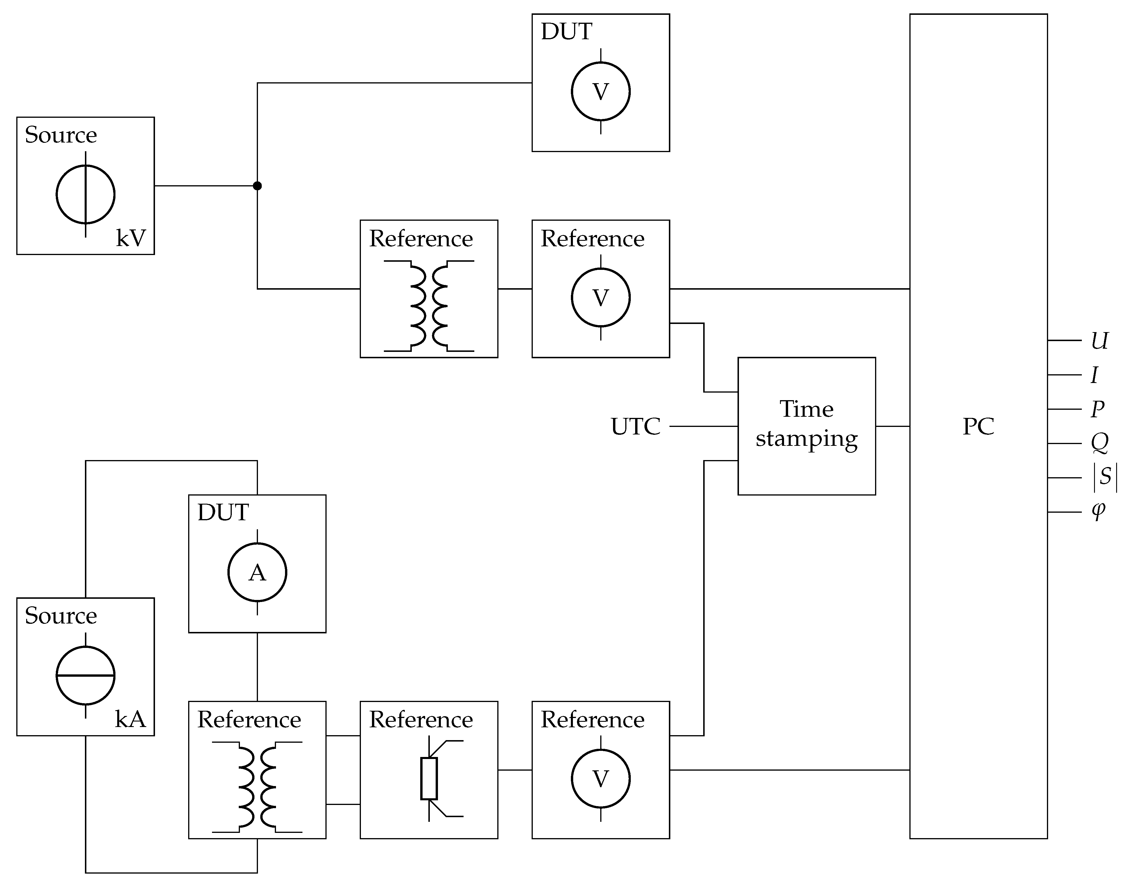
Figure 3.
Qualitative illustration: Short-term stability of the measurand and the importance of synchronisation of reference and dut. The quantitative impact strongly depends on the particular set-up and is very magnitude dependent. It needs to be evaluated for every individual case. While the principle applies to any measurand, the current is particularly liable to time dependency in this application, while the voltage is much more stable.


Table 1.
Uncertainty of shunt ac resistance.
| Source of Uncertainty | Standard Uncertainty in at Frequency | |||
|---|---|---|---|---|
| 50 Hz | 400 Hz | 1 kHz | 9 kHz | |
| DC resistance | 0.2 | 0.2 | 0.2 | 0.2 |
| AC-DC difference | 0.01 | 0.1 | 0.2 | 2 |
| Combined standard uncertainty | 0.2 | 0.3 | 0.3 | 2 |
Table 2.
Uncertainty of shunt phase.
| Source of Uncertainty | Standard Uncertainty in rad at Frequency | |||
|---|---|---|---|---|
| 50 Hz | 400 Hz | 1 kHz | 9 kHz | |
| Phase | 0.03 | 0.3 | 0.6 | 6 |
Table 3.
Comparison of voltmeter triggering modes.
| One Trigger | Internal | Equally | Predictable | Signal |
|---|---|---|---|---|
| Event | Clock | Spaced | Timing | Frequency |
| per | Sync. | Samples | Maintained | |
| sample | yes | yes | yes | yes |
| measurement | yes | yes | yes | yes |
| sample | no | no | no | yes |
| measurement | no | yes | no | no |
Table 4.
Uncertainty of the apparent power.
| Source of Uncertainty | Standard Uncertainty in at Frequency | |||
|---|---|---|---|---|
| 50 Hz | 400 Hz | 1 kHz | 9 kHz | |
| Voltmeter (voltage channel) | 5 | 10 | 100 | 150 |
| Voltmeter (current channel) | 5 | 10 | 100 | 150 |
| Shunt | 0.2 | 0.3 | 0.3 | 2 |
| Spread of the samples | 1 | 2 | 2 | 2 |
| Combined standard uncertainty | 7 | 14 | 142 | 212 |
| Expanded uncertainty (95%) | 15 | 30 | 300 | 500 |
Table 5.
Uncertainty of the displacement angle without a custom-designed Wagner earth circuit.
| Source of Uncertainty | Standard Uncertainty in rad at Frequency | |||
|---|---|---|---|---|
| 50 Hz | 400 Hz | 1 kHz | 9 kHz | |
| Phase displacement of shunt | 0.03 | 0.3 | 0.6 | 6 |
| Phase difference of voltmeters | 1 | 2 | 5 | 45 |
| Common mode voltage | 5 | 8 | 100 | 900 |
| Spread of the samples | 1 | 2 | 2 | 2 |
| Combined standard uncertainty | 6 | 9 | 100 | 900 |
| Expanded uncertainty (95%) | 11 | 17 | 200 | 1800 |
Table 6.
Uncertainty of the active and reactive power.
| Source of Uncertainty | Standard Uncertainty in at Frequency | |||
|---|---|---|---|---|
| 50 Hz | 400 Hz | 1 kHz | 9 kHz | |
| Combined standard uncertainty | 7 | 14 | 142 | 900 |
| Expanded uncertainty (95%) | 15 | 30 | 300 | 1800 |
Table 7.
Comparison results (120 V and 5 A).
| Settings | Difference | ||||
|---|---|---|---|---|---|
| Phase | Voltage | Current | Active | Reactive | Apparent |
| Power | Power | Power | |||
| 180 | 0 | −2 | 3 | 0 | −2 |
| 150 | 1 | −1 | 0 | −1 | −1 |
| 120 | 0 | −1 | 0 | −1 | −1 |
| 90 | 0 | 0 | 0 | −1 | −1 |
| 60 | 0 | 0 | −1 | 1 | 1 |
| 30 | 2 | 0 | 0 | 2 | 1 |
| 0 | 1 | 1 | 2 | −1 | 2 |
| −30 | 1 | 2 | 4 | −1 | 3 |
| −60 | 2 | 2 | 1 | −4 | 4 |
| −90 | 1 | 1 | 1 | −3 | 3 |
| −120 | 1 | 1 | −1 | −2 | 1 |
| −150 | -1 | 1 | −1 | 0 | 1 |
Table 8.
Comparison results (240 V and 5 A).
| Settings | Difference | ||||
|---|---|---|---|---|---|
| Phase | Voltage | Current | Active | Reactive | Apparent |
| Power | Power | Power | |||
| 180 | 2 | 1 | −2 | −2 | 2 |
| 150 | 2 | 2 | −4 | −2 | 4 |
| 120 | 2 | 1 | −4 | 1 | 2 |
| 90 | 1 | 1 | −4 | 2 | 2 |
| 60 | 2 | 0 | −1 | 3 | 2 |
| 30 | 2 | 1 | 2 | 3 | 3 |
| 0 | 2 | 2 | 3 | 2 | 2 |
| −30 | 1 | 1 | 3 | 0 | 3 |
| −60 | 3 | 2 | 4 | −2 | 4 |
| −90 | 1 | 2 | 3 | −2 | 2 |
| −120 | 2 | 2 | 1 | −6 | 5 |
| −150 | 2 | 1 | 0 | −4 | 3 |
Table 9.
Extended system: Uncertainty of the apparent power.
| Source of Uncertainty | Standard Uncertainty in at Frequency | |||
|---|---|---|---|---|
| 50 Hz | 400 Hz | 1 kHz | 9 kHz | |
| Voltmeter (voltage channel) | 5 | 10 | 100 | 150 |
| Voltage divider | 5 | 5 | 10 | 100 |
| Voltmeter (current channel) | 5 | 10 | 100 | 150 |
| Current transformer | 5 | 5 | 10 | 100 |
| Shunt | 0.2 | 0.3 | 0.3 | 2 |
| Spread of the samples | 1 | 2 | 2 | 2 |
| Combined standard uncertainty | 10 | 16 | 142 | 255 |
| Expanded uncertainty (95%) | 20 | 32 | 290 | 510 |
Table 10.
Extended system: Uncertainty of the displacement angle.
| Source of Uncertainty | Standard Uncertainty in rad at Frequency | |||
|---|---|---|---|---|
| 50 Hz | 400 Hz | 1 kHz | 9 kHz | |
| Phase displacement of voltage divider | 5 | 5 | 10 | 100 |
| Phase displacement of current transformer | 5 | 5 | 10 | 100 |
| Phase displacement of shunt | 0.03 | 0.3 | 0.6 | 6 |
| Phase difference of voltmeters | 1 | 2 | 5 | 45 |
| Spread of the samples | 1 | 2 | 2 | 2 |
| Combined standard uncertainty | 8 | 8 | 16 | 150 |
| Expanded uncertainty (95%) | 15 | 16 | 31 | 300 |
Publisher’s Note: MDPI stays neutral with regard to jurisdictional claims in published maps and institutional affiliations. |
© 2021 by the author. Licensee MDPI, Basel, Switzerland. This article is an open access article distributed under the terms and conditions of the Creative Commons Attribution (CC BY) license (https://creativecommons.org/licenses/by/4.0/).
Share and Cite
MDPI and ACS Style
Mester, C. Sampling Primary Power Standard from DC up to 9 kHz Using Commercial Off-The-Shelf Components. Energies 2021, 14, 2203. https://doi.org/10.3390/en14082203
AMA Style
Mester C. Sampling Primary Power Standard from DC up to 9 kHz Using Commercial Off-The-Shelf Components. Energies. 2021; 14(8):2203. https://doi.org/10.3390/en14082203
Chicago/Turabian StyleMester, Christian. 2021. "Sampling Primary Power Standard from DC up to 9 kHz Using Commercial Off-The-Shelf Components" Energies 14, no. 8: 2203. https://doi.org/10.3390/en14082203
Note that from the first issue of 2016, this journal uses article numbers instead of page numbers. See further details here.