Pore-Scale Simulation of Particle Flooding for Enhancing Oil Recovery

Abstract

The particles, water and oil three-phase flow behaviors at the pore scale is significant to clarify the dynamic mechanism in the particle flooding process. In this work, a newly developed direct numerical simulation techniques, i.e., VOF-FDM-DEM method is employed to perform the simulation of several different particle flooding processes after water flooding, which are carried out with a porous structure obtained by CT scanning of a real rock. The study on the distribution of remaining oil and the displacement process of viscoelastic particles shows that the capillary barrier near the location with the abrupt change of pore radius is the main reason for the formation of remaining oil. There is a dynamic threshold in the process of producing remaining oil. Only when the displacement force exceeds this threshold, the remaining oil can be produced. The flow behavior of particle–oil–water under three different flooding modes, i.e., continuous injection, alternate injection and slug injection, is studied. It is found that the particle size and the injection mode have an important influence on the fluid flow. On this basis, the flow behavior, pressure characteristics and recovery efficiency of the three injection modes are compared. It is found that by injecting two kinds of fluids with different resistance increasing ability into the pores, they can enter into different pore channels, resulting in the imbalance of the force on the remaining oil interface and formation of different resistance between the channels, which can realize the rapid recovery of the remaining oil.

1. Introduction

Water flooding is a primary measure for enhancing oil recovery in the oil development. However, in the water flooding process, water flows along the pore channels with smaller resistance. The pore radius, flooding velocity and fluid viscosity determine pore channel resistance characteristics. With oil development in depth, the oil phase in the channels is continuously displaced. The original oil-bearing channel is occupied by water, and the resistance further decreases, resulting in formation of high-permeability channels and a decrease of production efficiency. By injecting the particles into the pores, the resistance in the water-bearing high permeability channels is increased and the water is forced to flow to the low resistance channel, leading to utilization of residual oil and enhanced oil recovery [1,2,3]. However, the production efficiency varies with different displacement methods and displacement agents [4,5]. Investigation of the flow behaviors of particle–oil–water in the underground porous media is essential for optimizing the operation measure to recover the remaining oil efficiently.

Due to restriction of the technology of measurement in porous media, the dynamic mechanism of oil, water and particles in rock pore channels is studied mainly by numerical simulation, especially macrosimulation. However, the macroscale simulation results often fail to reveal the microflow mechanism and flow law of oil, water and particles in the pore channel and quantitatively analyze the flow path and flow pattern. With the development of computer technology, more and more researchers study the multiphase interaction mechanism in microstructure by numerical simulation [6,7,8,9]. However, the physical model of rock pore structure is too complicated to create a mathematical model. The difficulties include (1) real rock pore structure modeling: it is necessary to collect the real core and obtain the rock pore structure by CT scanning technology, and further acquire the physical structure of computational domain required for numerical simulation by image processing technology [10,11]; (2) no coupled mathematical model in the commercial software for description of two-phase mathematical model (VOF) in Eulerian framework and particle dynamics model in Lagrangian framework; (3) direct numerical simulation of interaction between particles and fluid: the particle size is far smaller than mesh scale; assuming that the particles have no size and the force of fluid on the particles is on the material points in the centers of the particles, the resistance source model is used to describe the interaction between the fluid and the particles; however, the particle size is larger than mesh scale, so the resistance source model is no longer applicable; thus it is necessary to calculate the interaction between the particles and the fluid by direct numerical simulation method [12].

Raeini et al. [13] studied two-phase flow by VOF, analyzed the control mechanism of two-phase flow and the effect of pore pressure at the pore scale, and carried out numerical simulation of two-phase flow in simple geometry structure. Kokubun et al. [14] simulated the migration behavior of the particles in porous media. The numerical results show that heterogeneous media present significant accumulation in low and high-velocity regions, whereas homogeneous media present only significant accumulation in low-velocity regions. Kokubun et al. [15] developed a simple model for the transport of polymer particles in an oil and water flow in a porous medium, which takes into account the clogging/unclogging of pore throats. Based on the Eulerian and Lagrangian frameworks, Su et al. [16] developed a VOF-FDM-DEM (VOF: volume-of-fluid, FDM: fictitious-domain-method and DEM: discrete element method) coupled method to simulate the particle flooding process and carried out the numerical test. Numerical results show that in the particle flooding process, three different stages, i.e., drainage period, analogy water flooding period and effective period of particle flooding, are involved. The oil recovery rate is closely related to the fluctuation of pressure difference between the inlet and outlet. However, the dynamic reason for startup of the residual oil in particle flooding after water flooding is unknown. What controls the particle–oil–water flow behaviors in particle flooding with different strategies, and how to choose the appropriate strategy for rapid and efficient oil recovery needs to be further investigated.

In this paper, the newly developed VOF-FDM-DEM coupled model [16] is employed to investigate the pore-scale particle–oil–water flow behaviors in the several different particle flooding processes. A new physical model scanned from a real rock through CT technology is constructed, and used in the simulation. The work is arranged as follows, the model details are given in the next section, followed by the case setup in the numerical tests used in the work. Results and discussions are presented in Section 4 and conclusions are drawn in Section 5.

2. Mathematical Model

VOF-FDM-DEM coupling method is a pore scale direct simulation method in the Eulerian–Lagrangian framework for particle flooding. In this method, Navier–Stokes equation is used for water–oil motion in the Eulerian framework, VOF simulation method is used to track water–oil interface. Newton’s second law is used to track particle motion in pore space in the Lagrangian framework, discrete element method is used to evaluate the particle–particle interaction and particle–wall interaction so as to be able to consider the collision properties of viscoelastic particles, and fictitious domain method is used for evaluating fluid–particle interaction force [17].

2.1. Oil–Water Flow Dynamics

The dynamic behaviors of water–oil two-phase interface in pore structure were described by the VOF model [18]. The continuity equation and momentum equation are described in Equations (1) and (2), respectively

$$\nabla ·\mathit{u}=0$$

(1)

$$\frac{\partial {\rho }_f\mathit{u}}{\partial t}+\nabla \cdot \left({\rho }_f\mathit{u}\mathit{u}\right)-\nabla \cdot \left(\mu \tau \right)=-\nabla p+{\rho }_{f}g+\mathsf{\sigma }\mathrm{k}\mathit{n}{\sigma }_s$$

(2)

where $\mathit{u}$ is average velocity of two phases, $m\cdot s^{-1}$; ${\rho }_f$ is average density of two phases, kg·m⁻³; μ is average dynamic viscosity coefficient of two phases, Pa·s; p is dynamic pressure, Pa; g is acceleration of gravity, m·s⁻²; k is surface curvature, m⁻¹; n is normal direction of interface; ${\sigma }_s$ is surface Dirac function.

$$\chi ={\chi }_1\alpha +\left(1-\alpha -\beta \right){\chi }_s+\beta {\chi }_2$$

(3)

where ${\chi }_1$ represents the physical properties of water; ${\chi }_2$ represents the physical properties of oil; ${\chi }_s$ represents the physical property of particle phase. α represents the volume fraction of water phase; $\beta$ represents the volume fraction of oil phase. If α = 1 is satisfied, the cell is filled with water; if β = 1 is satisfied, the cell is filled with oil. If α = 0 and β = 0 are satisfied, the cell is occupied by the particles. Otherwise, the cell is filled with two or three phases. However, the phase distribution inside the cell cannot be obtained without reconstruction.

In Equation (2):

$$k=-\nabla ·\mathit{n}$$

(4)

$$\mathit{n}=\frac{\nabla \alpha }{\left|\nabla \alpha \right|}$$

(5)

The fluid volume transport equation is expressed as follows:

$$\frac{\partial \alpha }{\partial t}+\nabla ·\left(\mathit{u}\alpha \right)=0$$

(6)

2.2. Particle Dynamics

Based on Newton’s second law, the dynamical model for discrete phase is used to track the motion of each particle in the Lagrangian framework. The mathematical expression is given as follows:

$$m_i\frac{d{\mathit{V}}_i}{dt}={\mathit{F}}_i^{p-p}+{\mathit{F}}_i^{w-p}+{\mathit{F}}_i^{f-p}+m_i\mathit{g}$$

(7)

where ${\mathit{F}}_i^{p-p}$ is the force between two particles, ${\mathit{F}}_i^{w-p}$ is the force acting on the particles from the wall, ${\mathit{F}}_i^{f-p}$ is the force of fluid on the i-th particle, m_i is the mass of the particle i, and g is the acceleration of gravity.

When the particles rotate, the moment on the i-th particle meets the following relationship:

$${\mathit{J}}_i\frac{d{\mathit{\omega }}_i}{dt}={\mathit{T}}_i^{p-p}+{\mathit{T}}_i^{w-p}+{\mathit{T}}_i^{f-p}$$

(8)

where J_i is the moment of inertia of the i-th particle, ω_i is the rotational angular velocity of the i-th particle, ${\mathit{T}}_i^{p-p}$ is the moment caused by the tangential force between particles, ${\mathit{T}}_i^{w-p}$ is the moment caused by the tangential force between the particle and the wall, and ${\mathit{T}}_i^{f-p}$ is the moment on the particle surface caused by fluid force.

Discrete element method is used to evaluate particle–particle ${\mathit{F}}_i^{p-p}$ and particle–wall ${\mathit{F}}_i^{w-p}$ contact forces. According to Cundall and Strack [19], the normal component of the contact force, ${\mathit{F}}_{nij}^{p-p}$ for particle–particle contact is

$${\mathit{F}}_{nij}^{p-p}=\left(-k_n{\mathit{\delta }}_n-{\eta }_n{\mathit{V}}_{ij}·\mathit{n}\right)\mathit{n}$$

(9)

and ${\mathit{F}}_{niw}^{w-p}$ for particle–wall contact is

$${\mathit{F}}_{niw}^{w-p}=\left(-k_{nw}{\mathit{\delta }}_{nw}-{\eta }_n{\mathit{V}}_{iw}·{\mathit{n}}_w\right){\mathit{n}}_w$$

(10)

In tangential direction, particle–particle interaction, ${\mathit{F}}_{tij}^{p-p}$, is

$${\mathit{F}}_{tij}^{p-p}=-k_t{\mathit{\delta }}_t-{\eta }_t{\mathit{V}}_{tij}$$

(11)

and ${\mathit{F}}_{tiw}^{w-p}$ for particle–wall interaction

$${\mathit{F}}_{tiw}^{w-p}=-k_{tw}{\mathit{\delta }}_{tw}-{\eta }_{tw}{\mathit{V}}_{tiw}$$

(12)

where k_n (k_nw) and η_n (η_nw) are the stiffness coefficient and damping coefficient, respectively, for particle–particle (or particle–wall) interactions in the normal direction. k_t (k_tw) and η_t (η_tw) are those in the tangential direction. δ_n(w) is particle–particle (or particle–wall) overlap in the normal direction. ${\mathit{\delta }}_{t\left(w\right)}$ is particle–particle (or particle–wall) displacement in the tangential direction. V_ij (V_iw) is the velocity of particle i relative to particle j (or wall), n_w is the vector pointing from the center of particle i to that of particle j (or the contact point on wall). The first item on the right hand side of the Equations (9)–(12) describes particle elastic behaviors and the second item describes the particle viscous behaviors.

If the tangential force and the normal force satisfy the following relation

$$\left|{\mathit{F}}_{tij\left(w\right)}^{p\left(w\right)-p}\right|\ge \chi \left|{\mathit{F}}_{nij\left(w\right)}^{p\left(w\right)-p}\right|$$

(13)

the particles (or particle–wall) in contact will slide against each other, and the tangential force is given as

$${\mathit{F}}_{tij\left(w\right)}^{p\left(w\right)-p}=-\chi \left|{\mathit{F}}_{nij\left(w\right)}^{p\left(w\right)-p}\right|\frac{{\mathit{\delta }}_{t\left(w\right)}}{\left|{\mathit{\delta }}_{t\left(w\right)}\right|}$$

(14)

where χ is the frictional coefficient.

The moment is for particle–particle contact

$${\mathit{T}}_i^{p-p}={\displaystyle \sum }_j{r}_{iC}\times {\mathit{F}}_{tij}^{p-p}$$

(15)

and for particle–wall contact

$${\mathit{T}}_i^{w-p}={\displaystyle \sum }_j{r}_{iC}\times {\mathit{F}}_{tij}^{w-p}$$

(16)

where, r_ic is the vector point from the contact point to the particle center.

A more elaborate description of the discrete element model can be found in our previous work [20]. Determination of the physical parameters, such as stiffness coefficient and damping coefficient, can be found in Tsuji et al. [21]. In this work, No-Binary-Search (NBS) algorithm is employed to find candidate contact spheres for each sphere in the system [22]. What is more, the efficient RIGID (ERIGID) algorithm [23] is used to judge the contact states between particles and pore walls.

2.3. Fictitious Domain Method for Fluid–Particle Interaction Force

In the particle flooding process, the particle diameter is generally similar to or larger than the throat diameter. The mesh size used in the simulation should be much smaller than the throat size in order to capture more flow details. As a result, the drag model for particle point source in Lagrangian framework cannot be applied because of larger particle size than mesh scale in rock pore structure. Thus, it is necessary to utilize the direct numerical simulation method, fictitious domain method, whose core idea is to add a volume force density function to the particle covering domain, so that the fluid in D has the behavior characteristics of particle [24,25]. Thus, Equation (2) gives

$$\frac{\partial {\rho }_f\mathit{u}}{\partial t}+\nabla ·\left({\rho }_f\mathit{u}\mathit{u}\right)-\nabla ·\left(\mu \mathit{\tau }\right)=-\nabla p+{\rho }_{f}g+\mathsf{\sigma }k\mathit{n}{\delta }_s+\mathit{\lambda } \mathrm{in}D$$

(17)

where

$$\nabla ·\mathit{u}=0\mathrm{in}D$$

(18)

$$\mathit{u}={\mathit{V}}_i+\mathit{\Omega }\times \mathit{r}\mathrm{in}{P}_i$$

(19)

The particle phase equations are expressed as follows:

$${\rho }_f\underset{P_i}{\overset{}{{\displaystyle \int }}}\mathit{\lambda }\mathrm{d}x=\frac{{\rho }_f-{\rho }_P}{{\rho }_P}{m}_i\left(\frac{d{\mathit{V}}_{\mathit{i}}}{dt}-\mathbf{g}\right)+{\mathit{F}}_i^{p-p}+{\mathit{F}}_i^{w-p}$$

(20)

$${\rho }_f\underset{P_i}{\overset{}{{\displaystyle \int }}}\mathit{r}\times \mathit{\lambda }\mathrm{d}x=\frac{{\rho }_f-{\rho }_P}{{\rho }_p}\left({\mathit{J}}_i\frac{d{\mathit{\omega }}_i}{dt}\right)+{\mathit{T}}_i^{p-p}+{\mathit{T}}_i^{w-p}$$

(21)

where λ is the non-zero only in the particle covering domain, and r is the location vector relative to the particle center. A more elaborate description of fictitious domain method can be found in our previous work [17].

3. Physical and Numerical Conditions

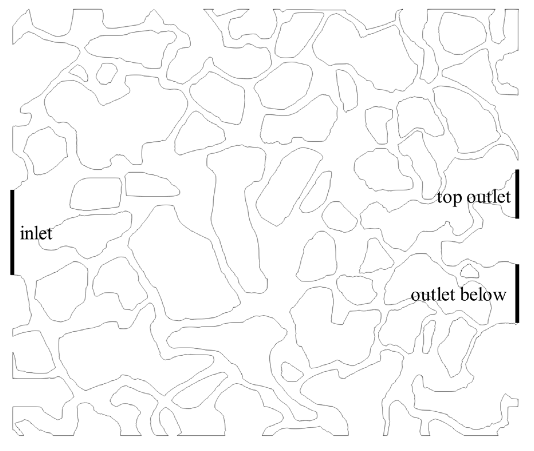
3.1. Physical Model and Case Setup

Figure 1 shows the two-dimensional physical model used in the simulation. It was obtained through CT scanning of a real rock. The inlet and outlet are shown in the figure. The physical model is 0.007315 m in length and 0.006175 m in width. The triangle unstructured mesh is used to divide pore space. The cell count is 254,155 in total. The maximum grid area is 1.19 × 10⁻¹⁰ m², and the minimum grid area is 1.40 × 10⁻¹¹ m². The minimum mesh size is much smaller than the particle size or pore size.

At first, the pore structure shown in Figure 1 was filled with oil, and water flooding was carried out until no oil flowed out from the outlet. Then, the newly developed VOF-FDM-DEM coupling model was used to simulate particle–oil–water flow process in particle flooding under various conditions. The description of each case is shown in

Table 1. Description of different test cases.

Item	Description	Time Interval (s)
Case I	Continuous injection of small particles	(0, 1) small particles
Case II	Continuous injection of big particles	(0, 1) big particles
Case III	Alternate injection of small and big Particles	(0, 0.5) small particles (0.5, 1) big particles
Case IV	Alternate injection of big and small particles	(0, 0.5) big particles (0.5, 1) small particles
Case V	Slug injection of small particles	(0, 0.5) small particles (0.5, 1) water
Case VI	Slug injection of big particles	(0, 0.5) big particles (0.5, 1) water

. Cases I and II are continuous injection, cases III and IV are alternate injection, and cases V and VI are slug injection. It is mainly divided into two kinds of particles. The physical parameters of particles and fluid are shown in

Table 2. Physical parameters used in particle flooding.

Item	Value
Particle density/kg·m−3	1000
Small particle size/m	10−4
Big particle size/m	5 × 10−4
Particle flow rate/kg·s−1	5 × 10−4
Normal/tangential stiffness coefficient/N·m−1	800/200
Normal/tangential damping coefficient/N·m−1	0.3/0.3
Friction coefficient	0.1
Water density/kg·m−3	1000
Water viscosity/kg·(m·s)−1	0.001
Water flow rate/m·s−1	0.01
Oil density/kg·m−3	800
Oil viscosity/kg·(m·s)−1	0.0148
Water oil interface tension/kg·s−2	0.07

.

3.2. Numerical Conditions

The numerical boundary conditions are given

Table 3. Numerical boundary conditions.

Physical Quantity	Boundaries
	Inlet	Outlet	Wall
Velocity	Fixed value	Zero gradient	Fixed value
Pressure	Zero gradient	Fixed value	Zero gradient
Water volume fraction	Fixed value	Zero gradient	Constant contact angle
Particle	Rebound	Exit	DEM

. Dirichlet boundary condition was employed for velocity at the inlet and the wall, for pressure at the outlet, for water volume fraction at the inlet. Neumann boundary condition was employed for velocity at the outlet, for pressure at the inlet and the wall, for water volume fraction at the outlet. Constant contact angle boundary condition was used for water–oil–solid contact line on the wall. Rebound boundary condition was used for particles at the inlet. Particles were allowed to exit from the outlet. Particle–wall interaction force was employed using discrete element method (DEM). Gamma Scheme presented in work was used to discretize the convection term [26,27] and Crank-Nicolson scheme was for the time term [28]. Leap-frog scheme is time discretization for particle tracking [29]. The residual errors of different physical quantities were set to 10⁻⁶. The courant number in the simulation was set to 0.1 and time step was adjusted adaptively [12].

4. Result and Discussion

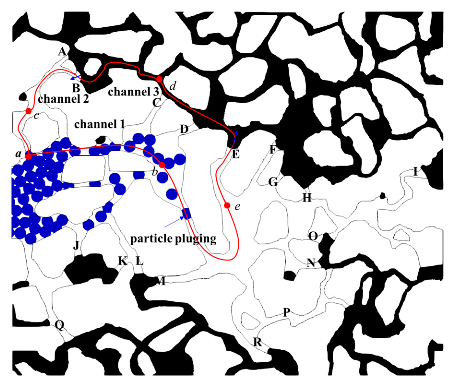
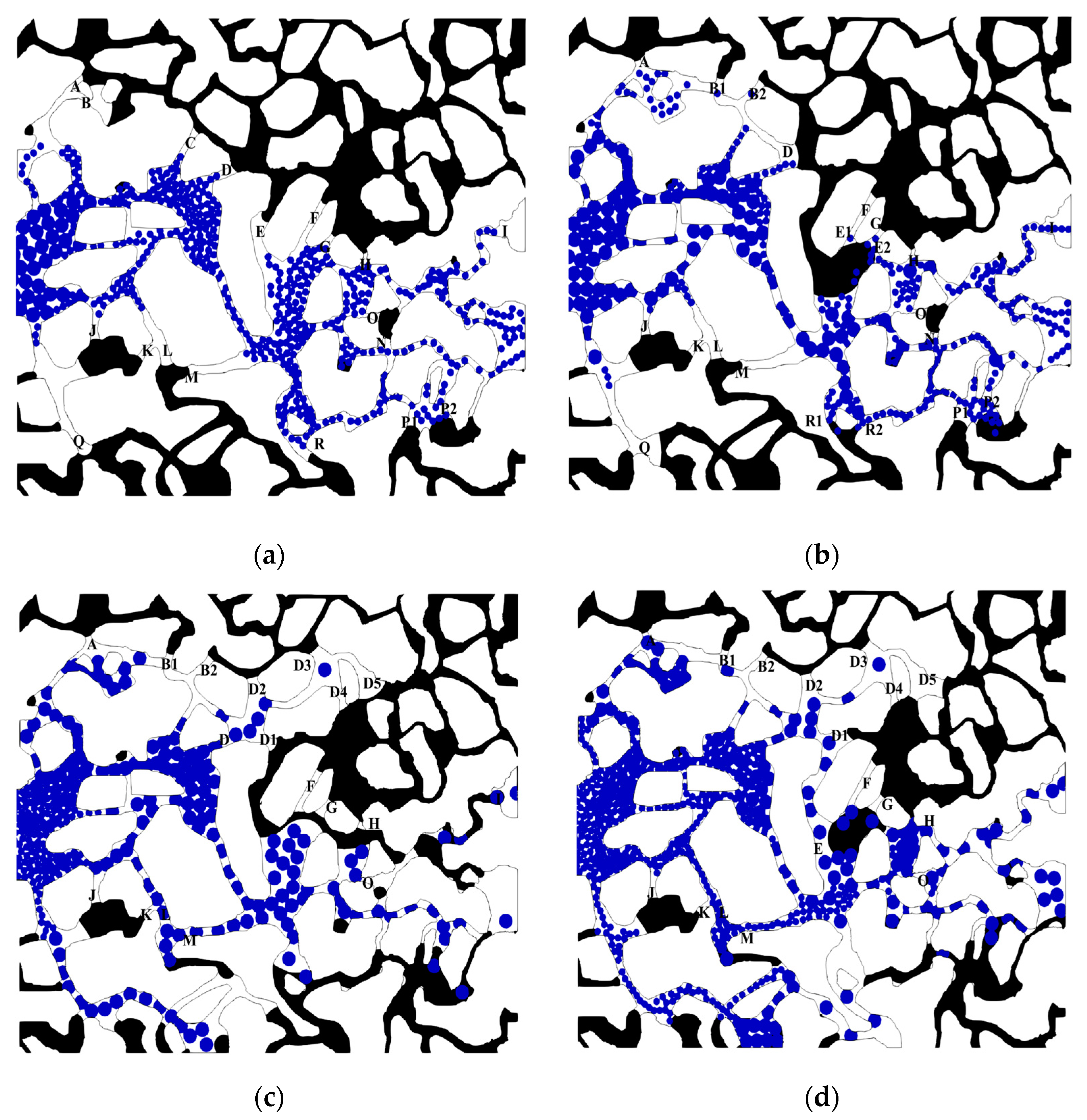
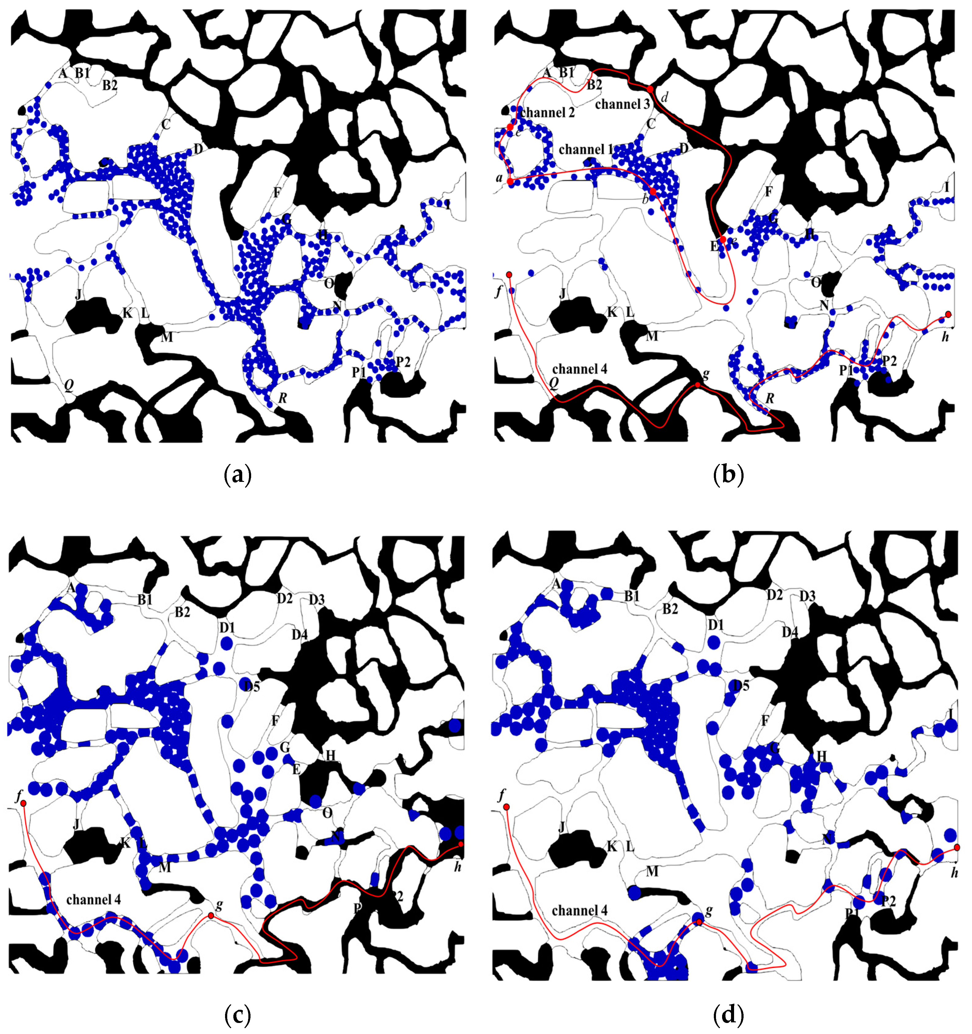
4.1. Trap Dynamics of the Residual Oil

The remaining oil distribution after water flooding is shown in Figure 2. The black line is the pore boundary, the white part in the pore is filled with water, and the black part is the remaining oil. Water flows in from the left and out from the two outlets on the right. It can be seen from the figure that the water cut channel is formed along the inlet and outlet direction after water flooding, and the remaining oil is mainly concentrated on both sides of the water cut channel.

The capital letters (A–R) in the figure indicate the location of the oil–water interface. It is not difficult to see that almost all the oil–water interface stays at the interface from throat to pore. At these locations, the pore radius changes greatly. In order to further describe the behavior of oil–water interface clearly, a simplified model is given in Figure 3, in which the black line is the pore boundary, the black part is oil, and the part not filled with color is full of water. $\varphi$ is the oil–water contact angle and $\psi$ is the opening angle from throat to pore. Figure 3a shows the situation of oil–water interface in the throat, when the capillary force caused by oil–water interface can be expressed by Laplace formula

$$f=\frac{\sigma cos\left(\varphi \right)}{R}$$

(22)

σ is the interfacial tension coefficient and R is the pore channel radius. Under water wet condition, the contact angle 𝜙 is an acute angle, and the f direction is consistent with the movement direction of water flooding, which is the driving force of water flooding. Figure 3b shows the situation of oil–water interface at the location throat entering the pore. After that, the oil–water interface will keep contact angle $\varphi$ with the pore wall, and the capillary force caused by the oil–water interface is

$$f=\frac{\sigma cos\left(\varphi +\psi \right)}{R}$$

(23)

When $\varphi +\psi$ > 90°, the oil–water interface will reverse. At this time, the capillary force obtained by Equation (23) is negative, which is opposite to the direction of water–oil displacement and hinders the movement of oil–water. As the oil–water interface moves forward, R will gradually increase, and the blocking effect of capillary force on oil–water interface will gradually decrease. When the oil–water interface flows out of the throat before entering the hole, the capillary force has a negative maximum. When the displacement force is insufficient to overcome the capillary pressure, the movement of oil–water interface stops. As a result, the oil in this channel cannot be exploited further. When water–oil interface passes a location with the abrupt change of pore radius, the capillary pressure can hinder the water–oil movement. This capillary resistance is called capillary barrier in this work. Capillary barrier is caused by abrupt change of pore radius, even in the water wet condition, capillary force caused by water–oil surface tension can still present resistance to water–oil movement. From the Equation (23), for specific pore structure, capillary barrier has a maximum value. When the hydrodynamic force does not exceed the extreme value of capillary barrier, the oil–water interface only deforms, but does not move. Once the displacement force exceeds the maximum value, the capillary force will be reduced or change its direction, so the difficulty of water flooding will be reduced.

In particular porous media, oil–water distribution affects the channel resistances distribution. Thus, the difference in the oil–water distribution will result in different displacement force in constant velocity flooding. Generally speaking, the viscosity of oil is higher than that of water. When the channel is occupied by one phase fluid, its resistance to the water flow is smaller than that of the oil flow. The displacement pressure required to maintain the process with the same flooding velocity will be reduced. Therefore, in the process of constant speed water flooding, the pressure difference between the inlet and outlet decreases with the increase of water saturation. The decrease of pressure difference results in the decrease of water displacement ability. Figure 2 shows the distribution of remaining oil after water flooding, and A–R is the position of oil–water interface. The channel from point a through point B to point E is called channel 1, the channel from point a through point C to interface B is called channel 2, and the channel from interface B through point D and interface E to point E is called channel 3. The pressure drop from point a to point e through channel 1 should be consistent with that from point a to point e through channels 2 and 3. As the remaining oil is in a static state, the fluid in channels 1 and 3 does not move, and there is no pressure drop in the channel from point a to the water side of interface B and the channel from point e to the water side of interface E. There is no pressure drop in channel 3 from oil side of interface B to oil side of interface E. Therefore, the pressure drop in channel 1 should be balanced with the sum of capillary forces caused by interfaces B and E. There is a maximum of capillary barrier at interface B; interface E moves from pore to throat, which is in the state of oil displacement, causing a resistance; as a result, the pressure drop in channel 1 must exceed the sum of the two resistances before the oil in channel 3 starts up. Therefore, the pressure difference between the interfaces is not enough to overcome the capillary pressure, which is the primary reason for the formation of residual oil.

4.2. Start-Up of the Remaining Oil in Particle-Flooding Process

When the particles are continuously injected into the porous structure after water flooding (case II) as shown in Figure 2, it is found that interfaces B and E begin to move after the time of 0.21 s, and the spatial distribution of particles–oil–water is shown in Figure 4 at 0.26 s. The capillary pressure caused by interfaces B and E points to the concave side, which hinders the movement of oil and water. At this time, there are particles migrating in channel 1, but there are no particles in channels 2 and 3 due to the plugging of channel by residual oil. Generally speaking, in the process of moving the remaining oil, the particles did not contact with the oil. This is due to the fact that the particles are carried by the water, and the resistance from pore walls to water is smaller than that that to the particles. As a result, the particles move behind the water–oil interface in the whole view.

In order to clarify the dynamic mechanism of residual oil recovery in the process of particle flooding, we probed the pressure of the water side of oil–water interface of A-I before and after the start-up of residual oil movement, and the results are shown in Figure 5. It can be seen from the figure that the water pressure near interfaces A and B is basically the same and shows an upward trend with time. At 0.21 s, the water phase pressure near interfaces A and B rises to a certain value, and interfaces B and E begin to move. At this time, the pressure transfer in channels 2 and 3 changes from static pressure transfer to dynamic pressure transfer, and channel 2 produces pressure loss, resulting in the decrease of water phase pressure near interfaces A and B. At the same time, there are particles flowing into the pores from the inlet, and the pressure at the point a increases with the increase of inlet pressure, which makes the water phase pressure near interfaces A and B increase. The combined results of the two actions make the water pressure near the interfaces A and B reach the minimum value in about 0.22 s, and then rise. At 0.26 s, there is a particle in channel 1 plugging the pore (as shown in Figure 4), resulting in the increase of pressure in the upstream part of the plugging position. For example, the water phase pressure near interfaces A, B, C and D will increase, but it will not affect the pressure in the downstream channel. As a result, the water phase pressure near interfaces E, F, G and H will not change. The pressure drop along channel 1 increases due to the viscosity increasing effect of the particles in channel 1 on the injection system and the plugging effect of the fluid caused by the interaction between the particles and the wall. When the pressure drop exceeds the capillary effect of interfaces B and E, the oil in channel 3 will start to move. Therefore, by increasing the resistance of the channel with water, particle flooding changes the spatial distribution and transmission direction of pressure, destroys the mechanical balance of oil–water interface in different channels of remaining oil, and promotes the movement of oil–water interface, thus producing the remaining oil.

It should be pointed out that due to the extreme value of capillary barrier, when the water phase pressure difference at different interfaces is lower than a certain limit value, the oil–water interface will only deform and change the capillary force to counteract the oil–water pressure difference, and the oil–water interface will not move at this time. When the water phase pressure difference of different interfaces is higher than this limit value, the oil–water interface will move, and the remaining oil will be recovered. Once the oil–water interface moves, the capillary pressure barrier will be destroyed, and the resistance of oil–water movement will be reduced. Therefore, there is a threshold in the process of producing the remaining oil. Only when the displacement force exceeds this threshold, the remaining oil can be produced. The threshold is directly related to capillary barrier.

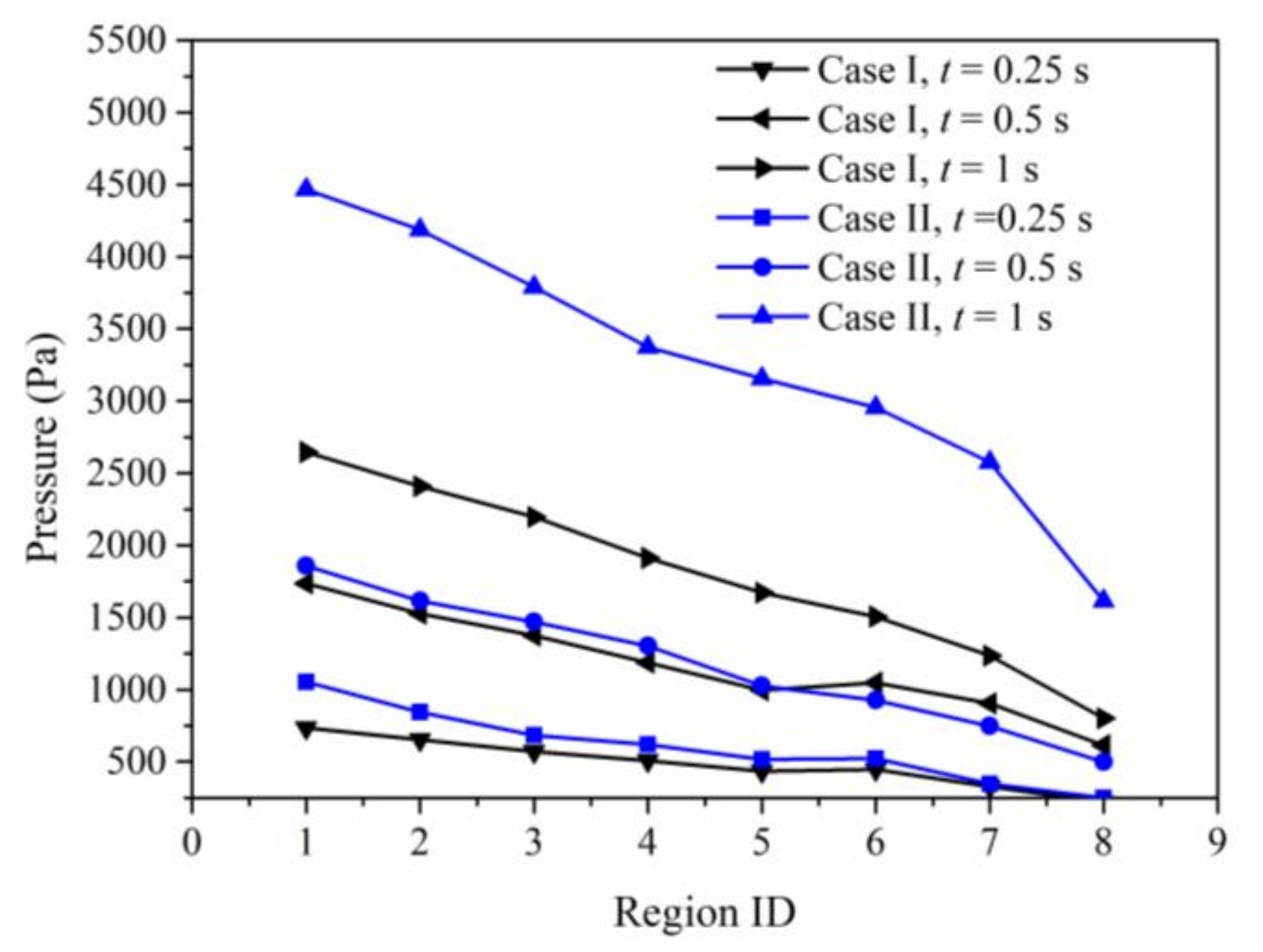
4.3. Effect of the Particle Size on Particle–Oil–Water Flow Behaviors

Particle size has an important influence on the behavior of particle–oil–water. For this reason, we continuously injected two different sizes of particles into the porous structure after water flooding as shown in Figure 2. At 0.5 and 1 s, the particle–oil–water distribution is shown in Figure 6.

At first, both small and large particles migrate along the channel with water, as shown in Figure 6a,c. The main reason is that:

• The viscosity of water is smaller than that of oil, and the resistance of water channel is smaller than that of oil channel. Therefore, the particles tend to move along the channel with low resistance.
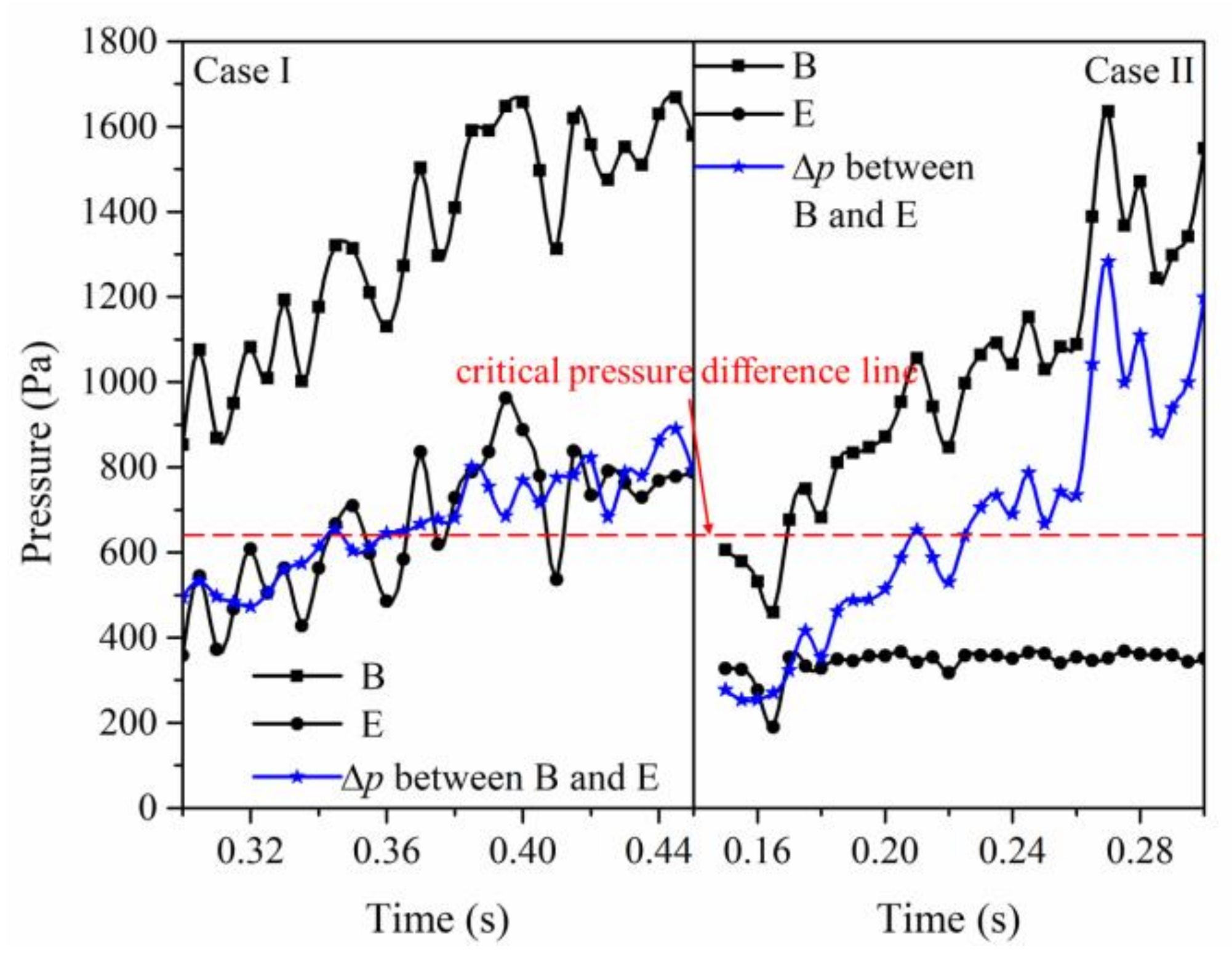
• There is a capillary barrier in the oil–water interface at the remaining oil boundary. When the displacement force is insufficient, the oil–water interface only deforms and does not move. At the beginning, there are few particles in the water channel, which cannot make enough pressure drop between different oil–water interfaces and the remaining oil remains stationary. These channels are blocked by static remaining oil, so that particles can only migrate in water channels.

With the increase of the number of injected particles, the residual oil in porous media can be produced by continuous injection of large particles or small particles. However, there are differences in the time when residual oil begins to move and in the final state of oil–water distribution. According to the particle–oil–water distribution given in Figure 6a at 0.5 s in case I (continuous injection of small particles), the remaining oil in channel 3 has just started to move at this time, while the remaining oil in channel 3 has been displaced from the channel in case II (continuous injection of large particles) at this time as given in Figure 6c. Figure 7 shows the time-dependent variation of water phase pressure near interfaces B and E before and after the start-up of residual oil in channel 3. It can be seen from the figure that for the continuous injection of small particles, the water phase pressure near the interface e presents a fluctuating upward trend, while in case II, the water phase pressure is relatively stable. The main reason is that the small particles have migrated to the pores downstream of the interface when the interface E begins to move in case I, while the particles have not moved to the vicinity of interface E in case II. Before and after the interface moves, the water pressure at interface B is the same as that at the entrance point A. With the injection of particles, the pressure at interface B increases in both cases. It can be seen from the water phase pressure near the interfaces B and E that the pressure difference in case II rises faster than that in case I. The critical pressure difference required for recovering the remaining oil under the two conditions is the same. After the interfaces start to move, the pressure changes from static pressure to dynamic pressure, the pressure drop in the channel decreases firstly and then rises continuously.

With the continuous injection of particles, both small particles and large particles produce an accumulation effect in the pores, and the accumulation of particles has a different effect on the final remaining oil production. Figure 6b,d shows the distribution of particles–oil–water in the case I at 1 s, respectively. It can be seen from the figure that the accumulation effect of large particles is larger, and the recovery rate of the remaining oil is larger too. The primary reason is that the movement of particles with different sizes are responsible for different resistances to the flow. Due to the influence of the wall effect, the larger particles have a greater hindrance to the movement of the fluid in the water channel than the smaller particles, so a larger displacement force is needed to maintain its movement. Under the condition of constant displacement rate, the pressure drop from the inlet to the outlet changes in two cases are different as shown in Figure 8. It can be seen from the figure that at the beginning, the pressure drops in both cases remain relatively stable. In case II after 0.13 s, the pressure begins to rise and fluctuates greatly after 0.23 s. Whereas in case I, the pressure begins to rise after 0.21 s. Although there are fluctuations in the process of pressure rise in this case, the fluctuation magnitude is much smaller than that in case II. There are two primary effects when particles migrate in the porous media.

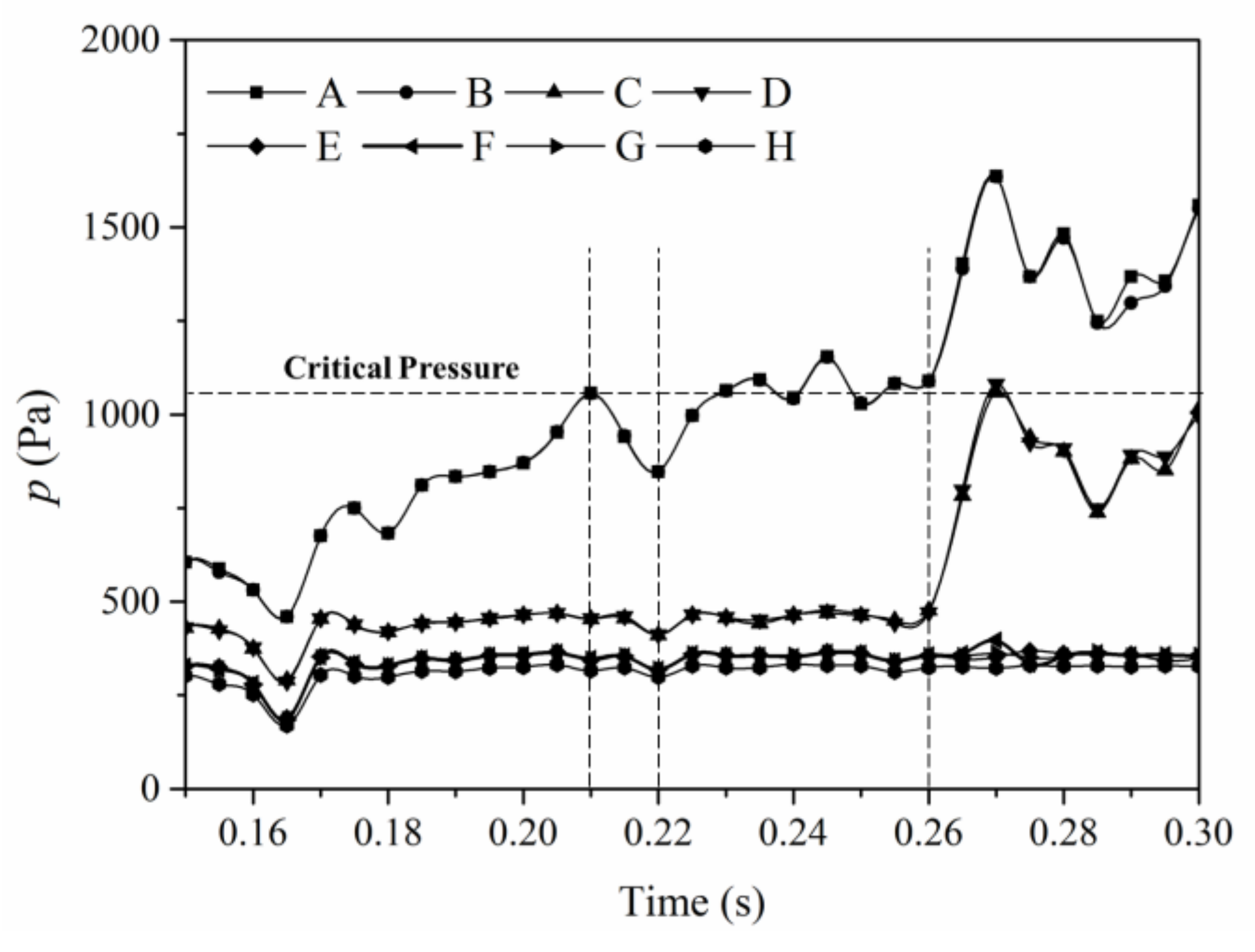
• The addition of particles to the displacement fluid will increase the effective viscosity of the displacement fluid. The higher the particle concentration, the greater the effective viscosity of the system. The larger the effective viscosity is, the more obvious the increase of channel resistance is. The viscosity effect will make the inlet–outlet pressure difference increase with time. With only the viscosity effect there will be no large pressure difference fluctuation in the rising process.
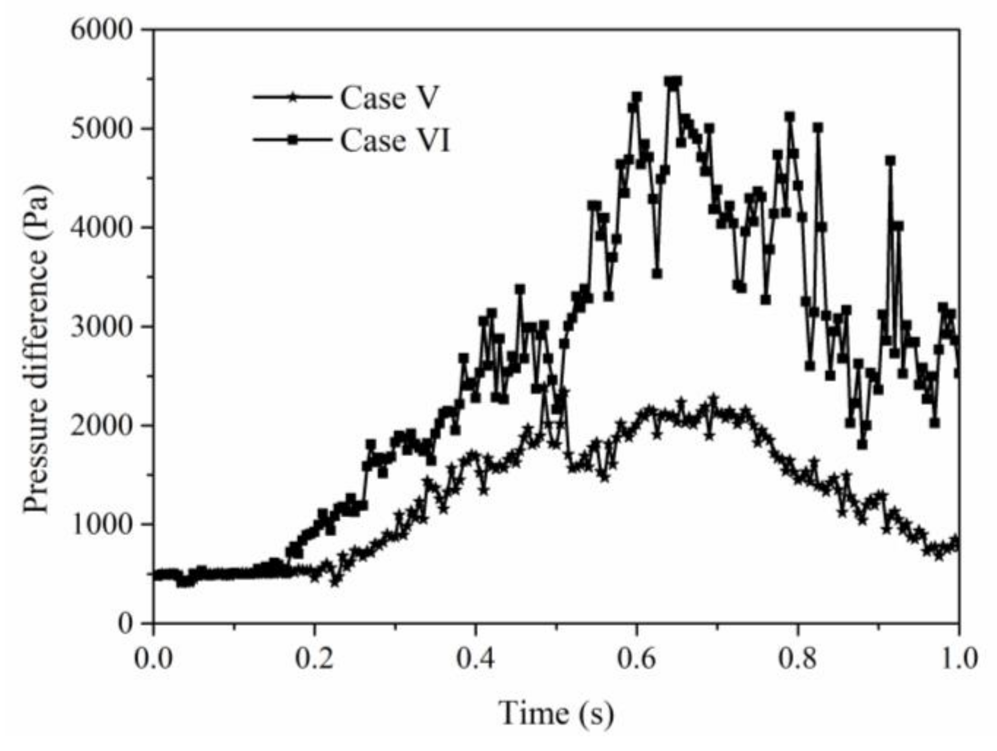
• When the particle size is larger than the pore size, the particle will block the pore channel. When plugging, the upstream pressure will rise rapidly; when breaking through, the upstream pressure will drop rapidly. The plugging and breakthrough of particles will cause a large pressure fluctuation in the process of particle migration.

It can be seen from variation of inlet–outlet pressure difference with time: in case I, the pressure rises, but the fluctuation is small, mainly due to viscosity increasing; in case II, the pressure difference rises and fluctuates greatly, and both viscosity increasing and plugging effect play an important role in the process of particle migration.

In order to study the pressure variation in the flow direction, we divided the computational area into eight zones along the flow direction and calculated the average pressure of each zone. The pressure distribution at different time is shown in Figure 9. It can be seen from the figure that with the advance of time, the pressure gradient between the inlet and outlet gradually increases with time. At 0.25 and 0.5 s, the accumulation of particles in the pores is relatively loose, and the pressurization effect of large and small particles has little difference. With the increase of accumulation degree, the pressurization effect of large particles is significantly enhanced, while the pressurization effect of small particles is not obvious. This is because in the case of small particles, the pressurization is mainly depending on increasing the effective viscosity, and there is a linear relationship between pressurization and particle concentration. However, for large particles, in the early stage, the concentration is low and the viscosity is dominant. In the later stage, with the increase of concentration, the plugging effect is obvious and the pressurization ability is significantly enhanced.

4.4. Particle–Oil–Water Behaviors in Different Particle Flooding Methods

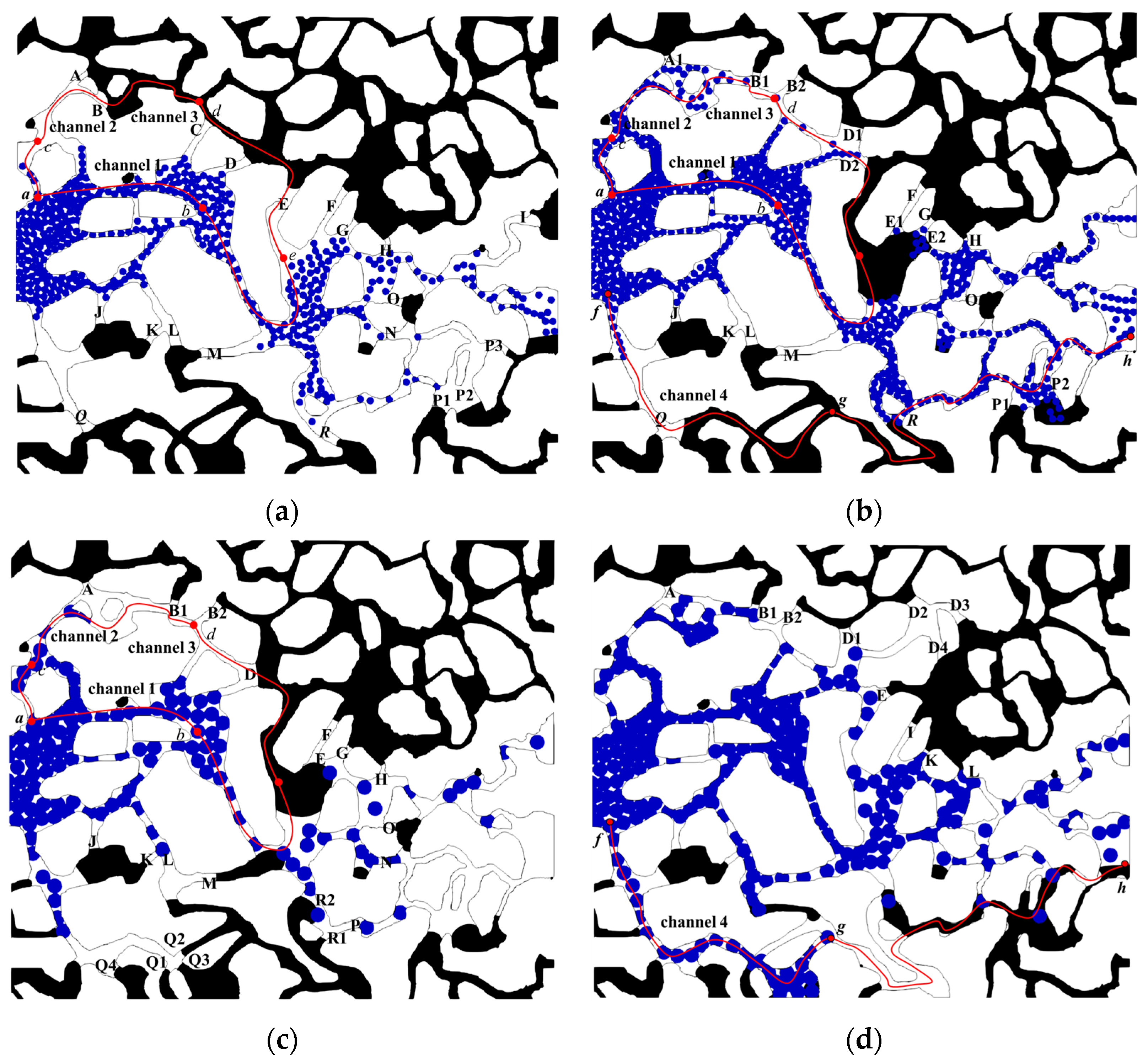
4.4.1. Alternate Injection of Big and Small Particles

The resistance increasing effect of particles with different size on the pore channel is different. When the particles are continuously injected into the channel, the initially injected particles will change the resistance of the channel, and they will flow to the channels with lower resistance. Therefore, the injection sequence of different size particles will have an impact on the spatial distribution of particles, and then affect the remaining oil production process, inlet–outlet pressure drop changes and the spatial distribution characteristics of pressure. Thus, we carried out the alternate injection of small and big particles in cases III and IV.

Figure 10 shows the spatial distribution of particles water and oil at different times in cases III and IV. It can be seen from the figure that in case III at 0.75 s, on the basis of the initial injection of small particles, large particles move along the water bearing channel, and move less toward the oil-bearing channel. The main reason is that the original injection of small particles did not pressurize the central water bearing channel enough, and the surrounding oil-bearing channels were blocked by capillary barrier, which limited the migration of particles to the surrounding oil-bearing channels. Later, with the injection of large particles, small particles are transported to the oil-bearing channel, and the final remaining oil production is not obvious, as shown in Figure 10b. At 0.75 s in case IV, due to the continuous injection of large particles in the early stage, the pores were sealed and the peripheral pore channels were opened by the residual oil production in the early stage. The particles formed a significant accumulation at the entrance and migrated to the surrounding pore channels at the same time. With the continuous injection of small particles, large particles are pushed to the oil-bearing channel. The production degree of the final remaining oil is higher than that of case III.

In order to further describe the difference of pore channel resistance increase in two different cases, this paper presents statistics on the change of inlet–outlet pressure difference with time in two cases, as shown in Figure 11. It can be seen from the figure that the pressure difference caused by the initial injection of small particles in case III is smaller than that caused by the injection of large particles in case IV; after the subsequent alternation of particles, case 2 can still maintain a higher inlet–outlet pressure difference, and the fluctuation amplitude of the pressure difference is higher than that in case 1. The pore structure is divided into eight zones along the flow direction, and the pressure of each zone is averaged, and the pressure change along the flow direction is obtained, as shown in Figure 12. It can be seen from the figure that in case III, with the continuous injection of large particles, the inlet–outlet pressure gradient gradually increases. At 1 s, the large particles did not migrate to the outlet, the average pressure of zones 7 and 8 changed little, and the increase of pressure gradient mainly concentrated between zones 1 and 6. For case IV, the continuous injection of small particles after the injection of large particles makes the overall pressure gradient change little, but the average pressure presents a downward trend. In this case, the large particles in the front hinder the path of the small particles, making the small particles behind more dense and the system maintains a higher pressure.

4.4.2. Slug Injection of Big or Small Particles

Slug injection is an important field operation mode. In order to study the particle–oil–water behavior in this way, the pore structure after water flooding shown in Figure 2 was slug injected with particles in cases V and VI. The distribution of particle–oil–water when injecting water in case V is shown in Figure 6a, and that in case VI is shown in Figure 6c.

Figure 13 shows the spatial distribution of particle–oil–water at different times under slug injection. For case V, only interfaces B and E move before water injection (Figure 6a) and 0.75 s (Figure 13a). From 0.75 to 1 s (Figure 13b), the remaining oil did not move. From 0.5 s, no residual oil flows out of the porous media. When the particles are continuously injected into the channel, the initially injected particles ones will change the resistance of the channel, and the ones will flow to the channels with lower resistance. In case VI, comparing the pre-water injection (Figure 6c) and 0.75 s (water injection 0.25 s, Figure 13c), it is found that the original interface D moves after water injection, and new interfaces D1, D2, D3 and D4 gradually form. At the same time, fluid in channel 4 shown in Figure 13c also moves, and with the increase of water injection, the remaining oil in this channel is further driven out.

Figure 14 shows the variation of the inlet–outlet pressure difference in cases V and VI with time. It can be seen from the figure that the pressure difference in both cases first increases and then decreases. In the process of rising and falling, there is fluctuation, and the fluctuation caused by large particles is larger than that caused by small particles. After water injection 0.5 s, the pressure rise can still maintain for a period of time, and then the pressure begins to decline.

The computational domain was divided into eight zones along the flow direction, and the average pressure of each zone was calculated to obtain the average pressure distribution as shown in Figure 15. It can be seen from the figure that the overall pressure first increases and then decreases in both cases. For case V, the overall pressure increases slightly in the first 0.25 s after water injection, and then decreases more in the following 0.25 s. For case VI, the increase of the overall pressure in the first 0.25 s is larger than that in the last 0.25 s. With the continuous injection of water, the pressure gradient formed between inlet and outlet gradually decreases.

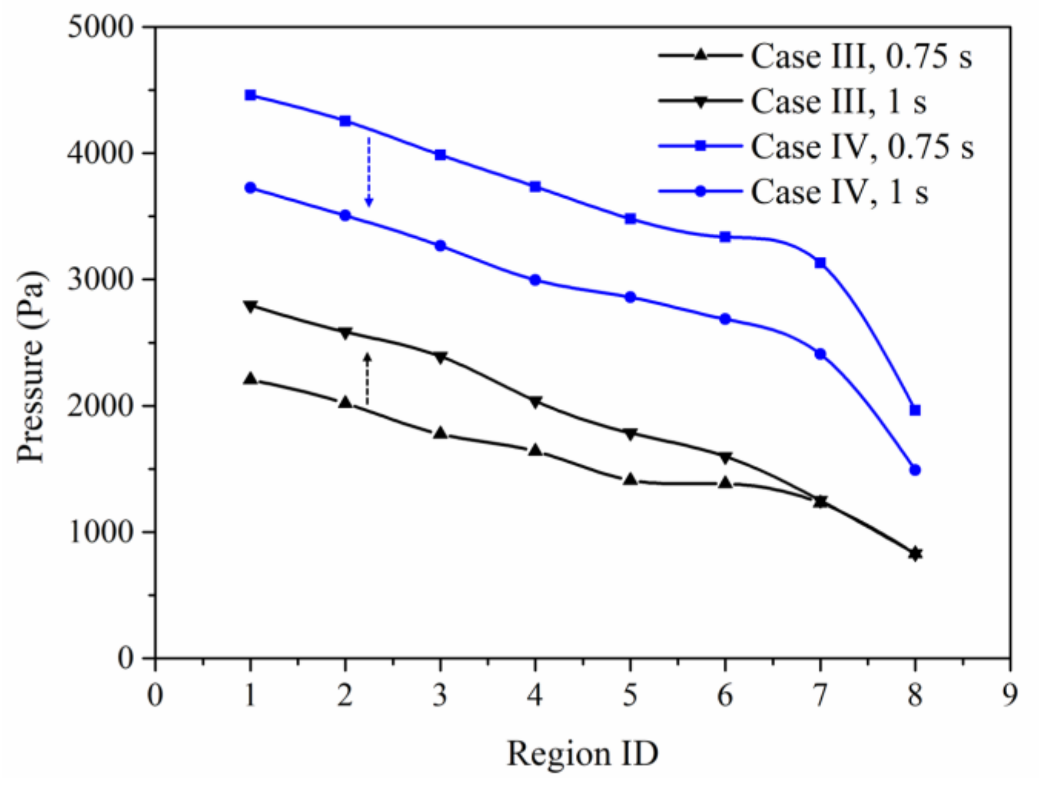
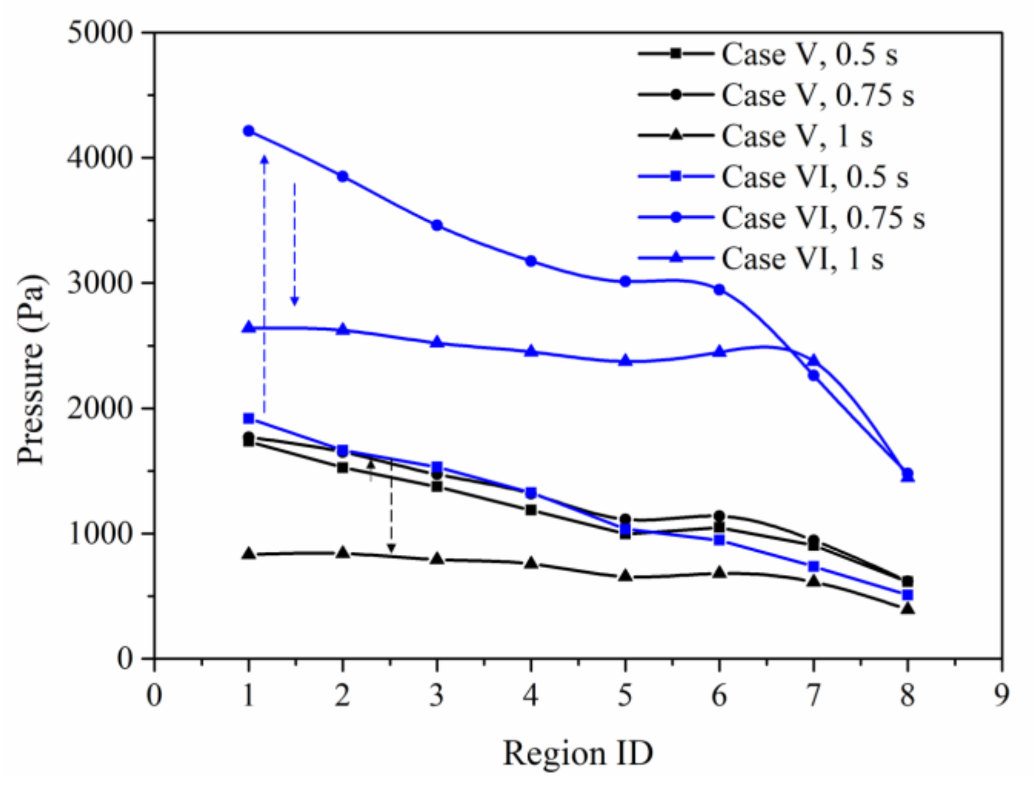
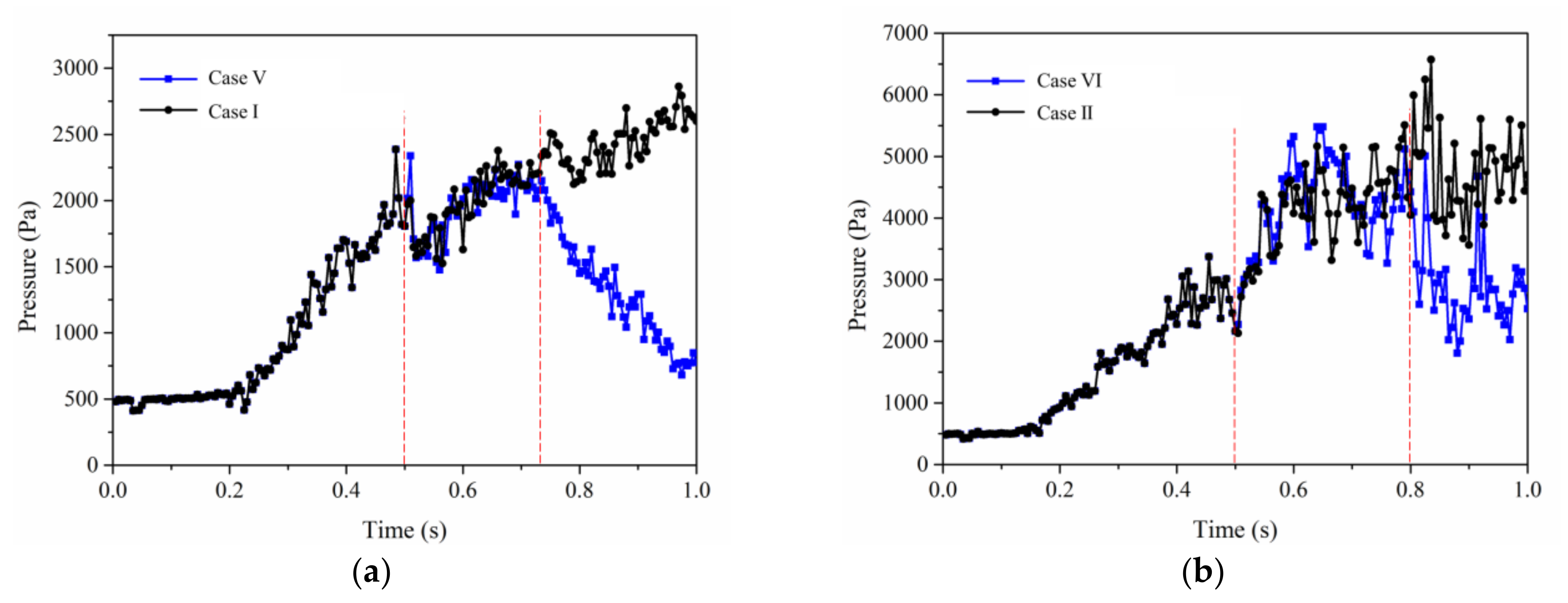
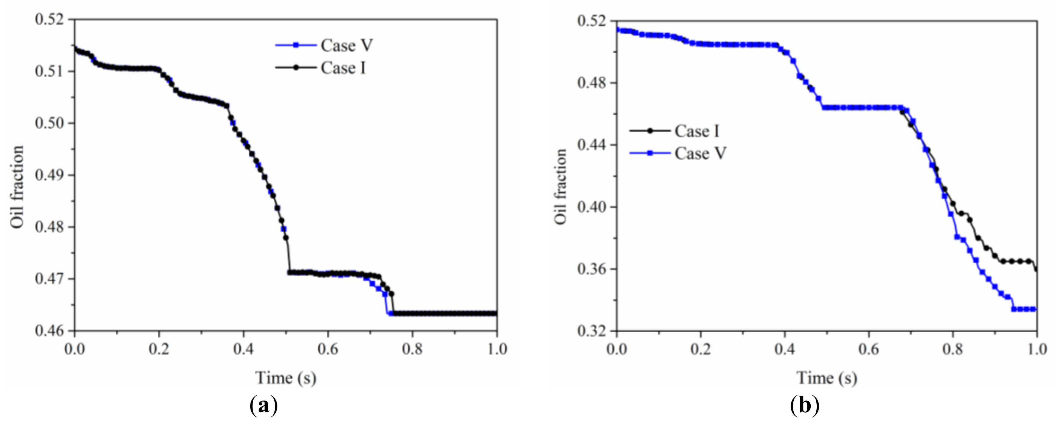
4.5. Comparison of Flow Behaviors among Different Flooding Methods

4.5.1. Flow Behaviors Comparison between Continuous Particle Injection and Slug Particle Injection

Figure 16 shows the comparison of the inlet–outlet pressure difference in continuous injection and slug injection with time. It can be seen from the figure that the pressure can still maintain for a certain period of time after replacement of water injection at 0.5 s. After water injection in case VI, the maintenance time of inlet–outlet pressure difference is longer than that of case V. From the beginning, the pressure difference drop rate in case V is larger than pressure difference increase rate in case I.

Figure 6b and Figure 13b show the particle–oil–water distribution with continuous small particle injection (case I) and slug small-particle injection (case V) at 1 s, respectively. Under the condition of continuous injection, the oil recovery in channels 3 and 4 is higher than that of slug injection. Figure 17a shows the oil saturation variation with time in two cases. It can be seen from the figure that the remaining oil of the two methods is basically the same at 1 s, and the time of remaining oil flowing out of the remaining oil under the condition of slug injection is earlier than that under the condition of continuous injection. Figure 6d and Figure 13d show the particle–oil–water distribution at 1 s for continuous big-particle injection (case II) and slug big-particle injection (case VI), respectively. Comparing the two cases, it is found that the oil recovery in channel 4 in case VI is larger than that in case II. This is mainly due to the accumulation of a large number of particles between F-G in channel 4 in case II (as shown in Figure 6d), which increases the drag in the driving process, weakens the driving force of the later produced oil, and reduces the flow speed of the remaining oil. Figure 17b shows the change of remaining oil in pore structure with time in cases II and VI. It can be seen from the figure that after 0.7 s, the remaining oil produced by slug injection of large particles is faster than that produced by continuous injection of large particles.

Therefore, in the process of injecting particles into porous media, the pressure difference between the inlet and outlet will rise. When the particles enter the channel parallel to the oil-bearing channel, the particles reduce the relative resistance of the oil-bearing channel by increasing the resistance of the channel, and finally increase the flow velocity of the remaining oil. When the particles enter the channel in series with the oil-bearing channel, by increasing the resistance of the channel, the relative resistance of the oil-bearing channel increases, and the partial flow of the oil-bearing channel decreases, resulting in the decrease of the production speed of the remaining oil. By injecting two kinds of media with different resistance increasing ability into the formation, the media with larger resistance can enter the water bearing channel, and the media with smaller resistance can enter the oil-bearing channel. The purpose of rapid movement of remaining oil can be achieved by adjusting the relative resistance of oil-bearing and water-bearing channels. Slug injection is closer to the target than continuous injection.

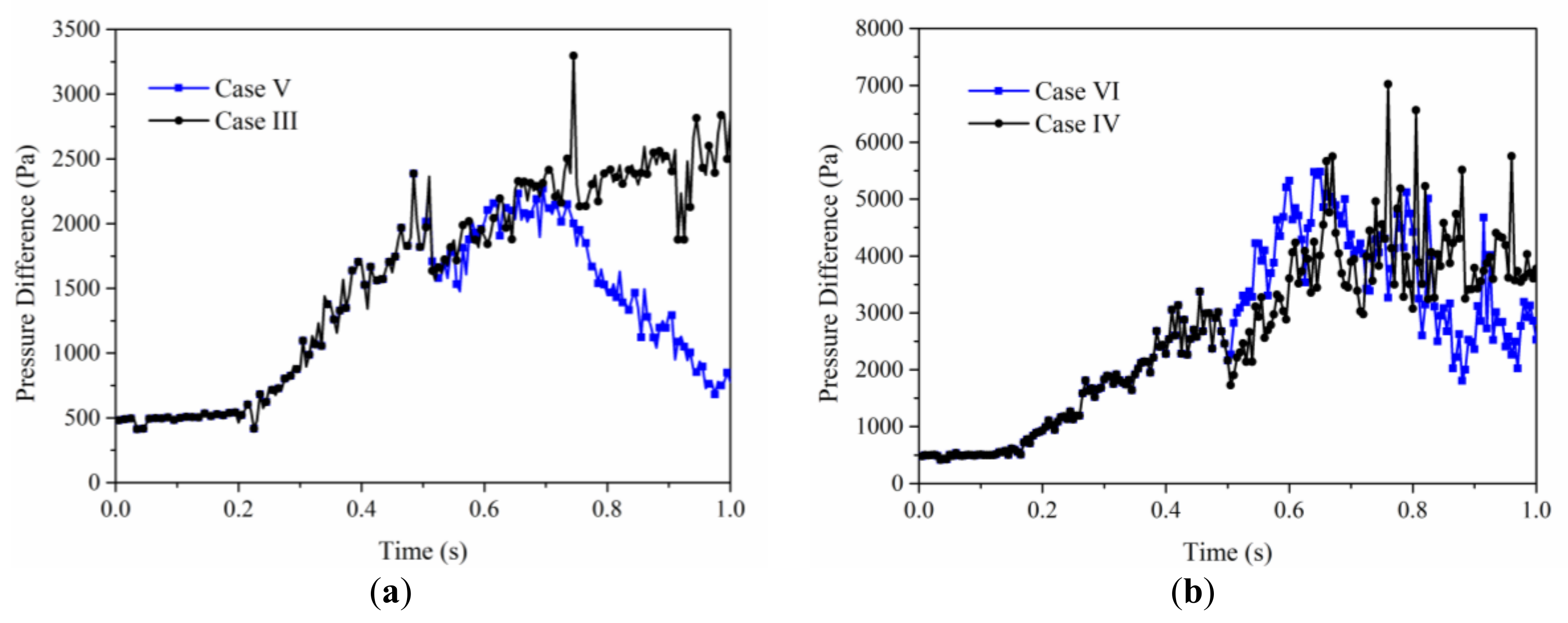
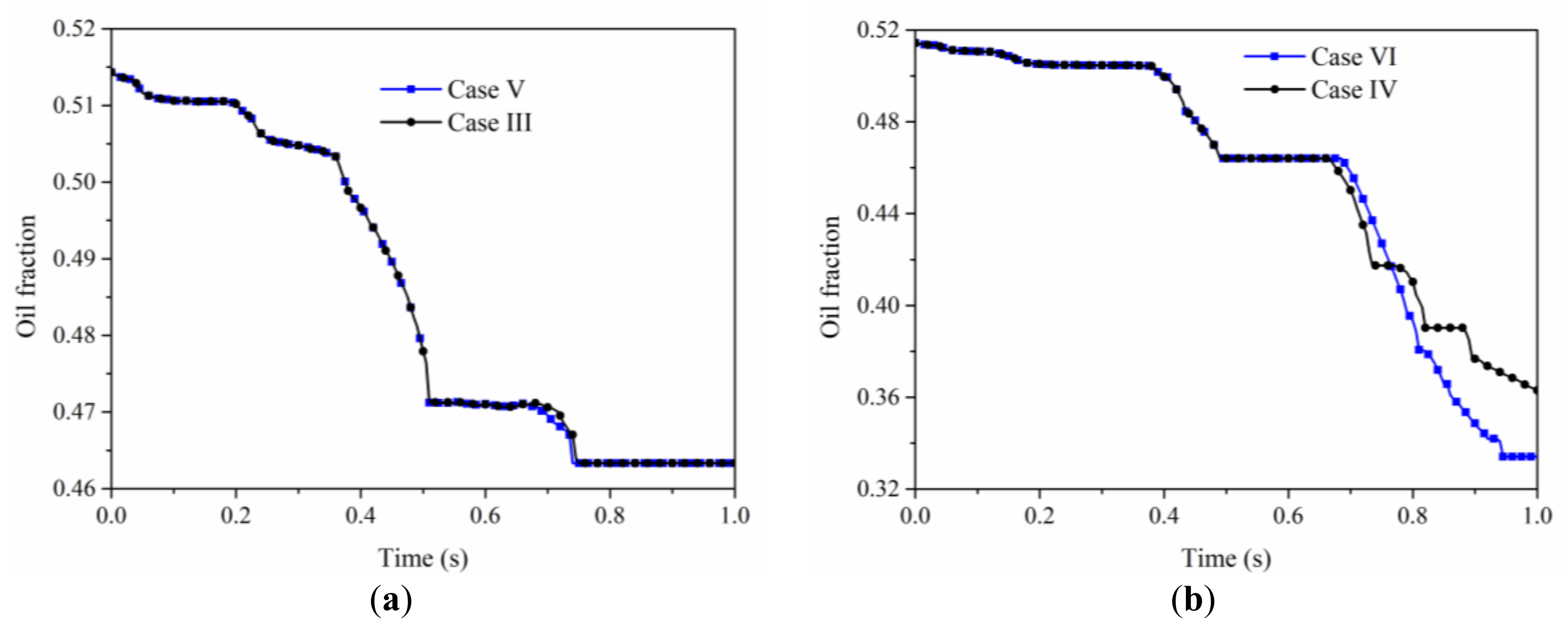
4.5.2. Multiphase Phase Behaviors Comparison between Continuous Particle Injection and Alternate Particle Injection

Figure 18a shows the time-dependent variation of the inlet–outlet pressure difference with continuous injection of small particles (case I) and alternate injection of small particles and large particles (case III). It can be seen from the figure that the variation of the inlet-outlet pressure difference with continuous injection of small particles is similar to that with alternate injection (from small particles to large particles). After injecting big particles, the pressure will not rise sharply in a short time. Figure 19a shows the change of oil saturation with time in pore structure in two cases. It is not difficult to see that the final remaining oil saturation of the two cases is the same, and the development speed of the remaining oil in the case of alternate injection is higher than that in the case of continuous injection.

Figure 18b shows the time-dependent variation of the inlet–outlet pressure difference with continuous injection of large particles (case II) and alternate injection of large particles and small particles (case IV). It can be seen from the figure that the pressure difference caused by continuous injection of large particles is slightly larger than that caused by alternate injection (from large particles to small particles). The pressure difference fluctuation is almost the same in both cases. From the change of oil saturation (as shown in Figure 19b), the final remaining oil saturation under the two conditions is consistent. However, the residual oil produced by alternate injection of particles (from large particles to small particles) is faster (more oil flows out in a short time), but its producing ability is worse than that by continuous injection (the residual oil continuously comes out of the pore structure under continuous injection, while the residual oil comes out intermittently under alternate injection).

It is easier to form resistance difference in water bearing and oil-bearing channels by injecting particles of different sizes alternately, so as to realize rapid production of remaining oil.

4.5.3. Multiphase Phase Behaviors Comparison between Slug Particle Injection and Alternate Particle Injection

Figure 20a shows the time-dependent variation of inlet–outlet pressure difference during slug injection of small particles (case V) and alternate injection of small particles to large particles (case III). It can be seen from the figure that from 0.5 to 0.7 s, the two injection methods have almost the same effect on the inlet–outlet pressure difference. After 0.7 s, the pressure difference continued to increase under alternate injection condition, while it continued to decrease under slug injection condition. The change of remaining oil saturation with time in pore structure under two production conditions is shown in Figure 21a. It can be seen that the final remaining oil with two methods is the same. In the process of slug injection, the resistance increasing ability of the injected fluid to the pore channel is different, so the slug injection can form the resistance difference in different channels and realize the rapid production of the remaining oil.

Figure 20b shows the variation of inlet–outlet pressure difference with time during slug injection of large particles (case VI) and alternate injection of large particles to small particles (case IV). It can be seen from the figure that the pressure difference with slug injection from 0.5 to 0.7 s is larger than that with alternate injection, and the pressure difference from 0.7 to 0.8 s in both cases is similar, and the pressure difference with slug injection after 0.8 s is smaller than that with alternate injection. It can be seen from the changes of oil saturation with time in the two processes shown in Figure 21b that slug injection can form better production speed and production capacity, and the final recovery rate is high. This is mainly due to the greater difference of resistance increasing ability of injected fluid to channel during slug injection, so the production effect is better.

5. Conclusions

In this paper, the pore-scale numerical simulation technology was used to carry out water flooding on the pore structure obtained from a real rock, and then different particle flooding development methods were used to displace the remaining oil after water flooding. The formation reasons of the remaining oil after water flooding, the dynamic mechanism of particle flooding, the multiphase hydrodynamic behavior of particle oil water under different sizes and injection methods, and their influencing factors were analyzed. The results are as follows:

(1)

When the pressure gradient gradually decreases so that the capillary resistance effect cannot be overcome, the movement of oil–water interface stops and the remaining oil is formed. There is a dynamic threshold in the process of producing remaining oil. Only when the dynamic threshold is exceeded can the remaining oil begin to move. In the process of particle flooding, the migration of particles in the water bearing channel increases the resistance of the water bearing channel, resulting in the formation of pressure difference at the water bearing side of different interfaces of the remaining oil. When the pressure difference exceeds the dynamic threshold, the remaining oil begins to move.

(2)

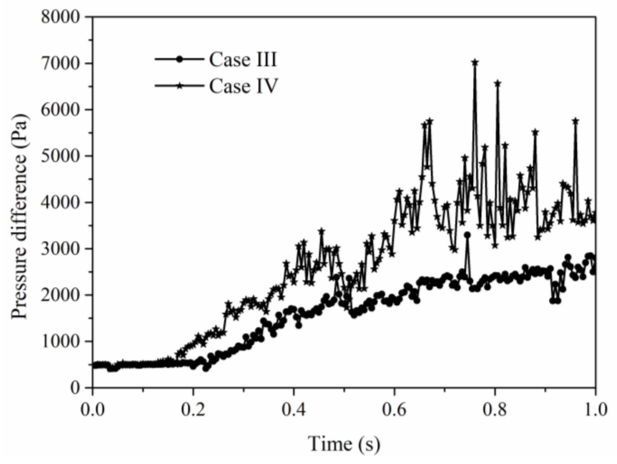
In the process of particle flooding, large particles can cause higher pressure difference rise and pressure difference fluctuation, and the remaining oil production capacity is higher than that of small particles. Therefore, the oil production time with large particles is smaller than that with small particles. The final remaining oil production is also higher than that of small particles.

(3)

Through the analysis and pairwise comparison of multiphase fluid behavior and remaining oil production characteristics under three injection modes of continuous injection, slug injection and alternate injection, it is found that when the fluid medium with different resistance increasing ability is injected into the pores, different fluids can enter into different pore channels, promote the imbalance of remaining oil interface, and achieve the purpose of rapid production of remaining oil. There is the biggest difference between the resistance increasing ability of large particles and water to pores. While reducing the average injection pressure, different resistance can be formed in different channels. Therefore, the ultimate recovery rate of slug injection of large particles is the highest.

References

1. Zhao, S.; Pu, W. Migration and plugging of polymer microspheres (PMs) in porous media for enhanced oil recovery: Experi-mental studies and empirical correlations. Colloid Surf. B 2020, 297, 124774. [Google Scholar] [CrossRef]
2. Lesin, V.I.; Koksharov, Y.A.; Khomutov, G.B. Magnetic nanoparticles in petroleum. Pet. Chem. 2010, 50, 102–105. [Google Scholar] [CrossRef]
3. Negin, C.; Ali, S.; Xie, Q. Application of nanotechnology for enhancing oil recovery—A review. Petroleum 2016, 2, 324–333. [Google Scholar] [CrossRef]
4. Foroozesh, J.; Kumar, S. Nanoparticles behaviors in porous media: Application to enhanced oil recovery. J. Mol. Liq. 2020, 316, 113876. [Google Scholar] [CrossRef]
5. Liu, D.; Gu, Z.; Liang, R.; Su, J.; Ren, D.; Chen, B.; Huang, C.; Yang, C. Impacts of Pore-Throat System on Fractal Character-ization of Tight Sandstones. Geofluids 2020, 9, 1–17. [Google Scholar]
6. Mack, J.C.; Smith, J.E. In-depth colloidal dispersion gels improve oil recovery efficiency. In Proceedings of the SPE/DOE Improved Oil Recovery Symposium, Tulsa, OH, USA, 17–20 April 1994. [Google Scholar]
7. Yuan, J.; Sundén, B. On mechanisms and models of multi-component gas diffusion in porous structures of fuel cell electrodes. Int. J. Heat Mass Transf. 2014, 69, 358–374. [Google Scholar] [CrossRef]
8. Akai, T.; Alhammadi, A.M.; Blunt, M.J.; Bijeljic, B. Modeling Oil Recovery in Mixed-Wet Rocks: Pore-Scale Comparison Be-tween Experiment and Simulation. Transp. Porous Med. 2019, 127, 393–414. [Google Scholar] [CrossRef] [Green Version]
9. Raeini, A.Q.; Bijeljic, B.; Blunt, M.J. Numerical modelling of sub-pore scale events in two-phase flow through porous media. Transp. Porous Med. 2014, 101, 191–213. [Google Scholar] [CrossRef]
10. Bijeljic, B.; Raeini, A.; Mostaghimi, P.; Blunt, M.J. Predictions of non-Fickian solute transport in different classes of porous media using direct simulation on pore-scale images. Phys. Rev. E 2013, 87, 013011. [Google Scholar] [CrossRef] [Green Version]
11. Su, J.; Wang, L.; Gu, Z.; Zhang, Y.; Chen, C. Advances in Pore-Scale Simulation of Oil Reservoirs. Energies 2018, 11, 1132. [Google Scholar] [CrossRef] [Green Version]
12. Su, J.; Chai, G.; Wang, L.; Cao, W.; Gu, Z.; Chen, C.; Xu, X.Y. Pore-scale direct numerical simulation of particle transport in porous media. Chem. Eng. Sci. 2019, 199, 613–627. [Google Scholar] [CrossRef]
13. Raeini, A.Q.; Blunt, M.J.; Bijeljic, B. Direct simulations of two-phase flow on micro-CT images of porous media and upscaling of pore-scale forces. Adv. Water Resour. 2014, 74, 116–126. [Google Scholar] [CrossRef]
14. Kokubun, M.E.; Muntean, A.; Radu, F.; Kumar, K.; Pop, I.; Keilegavlen, E.; Spildo, K.; Spildop, K. A pore-scale study of transport of inertial particles by water in porous media. Chem. Eng. Sci. 2019, 207, 397–409. [Google Scholar] [CrossRef] [Green Version]
15. Kokubun, M.A.E.; Radu, F.A.; Keilegavlen, E.; Kumar, K.; Spildo, K. Transport of Polymer Particles in Oil–Water Flow in Porous Media: Enhancing Oil Recovery. Transp. Porous Media 2018, 126, 501–519. [Google Scholar] [CrossRef] [Green Version]
16. Su, J.; Chai, G.; Wang, L.; Cao, W.; Yu, J.; Gu, Z.; Chen, C. Direct numerical simulation of pore scale particle-water-oil transport in porous media. J. Pet. Sci. Eng. 2019, 180, 159–175. [Google Scholar] [CrossRef]
17. Su, J.; Chai, G.; Wang, L.; Yu, J.; Cao, W.; Gu, Z.; Chen, C.; Meng, W. Direct numerical simulation of particle pore-scale transport through three-dimensional porous media with arbitrarily polyhedral mesh. Powder Technol. 2020, 367, 576–596. [Google Scholar] [CrossRef]
18. Ubbink, O. Numerical Prediction of Two Fluid Systems with Sharp Interfaces. Ph.D. Thesis, University of London, London, UK, 1997. [Google Scholar]
19. Cundall, P.A.; Strack, O.D.L. A discrete numerical model for granular assemblies. Géotechnique 1979, 29, 47–65. [Google Scholar] [CrossRef]
20. Su, J.; Gu, Z.; Xu, X.Y. Discrete element simulation of particle flow in arbitrarily complex geometries. Chem. Eng. Sci. 2011, 66, 6069–6088. [Google Scholar] [CrossRef]
21. Tsuji, Y.; Tanaka, T.; Ishida, T. Lagrangian numerical simulation of plug flow of cohesionless particles in a horizontal pipe. Powder Technol. 1992, 71, 239–250. [Google Scholar] [CrossRef]
22. Munjiza, A.; Andrews, K.R.F. NBS contact detection algorithm for bodies of similarsize. Int. J. Numer. Methods Eng. 2015, 43, 131–149. [Google Scholar] [CrossRef]
23. Su, J.; Huang, C.; Gu, Z.; Chen, C.; Xu, X. An Efficient RIGID Algorithm and Its Application to the Simulation of Particle Transport in Porous Medium. Transp. Porous Media 2016, 114, 99–131. [Google Scholar] [CrossRef]
24. Patankar, N.A.; Singh, N.A.; Joseph, D.; Glowinski, R.; Pan, T. A new formulation of the distributed Lagrange multipli-er/fictitious domain method for particulate flows. Int. J. Multiph. Flow 2000, 26, 1509. [Google Scholar] [CrossRef]
25. Patankar, N.A. A Formulation for Fast Computations of Rigid Particulate Flows; Center for Turbulence Research Annual Research Briefs: Stanford, CA, USA, 2001; pp. 185–196. [Google Scholar]
26. Jasak, H.; Weller, H.G.; Gosman, A.D. High resolution NVD differencing scheme for arbitrarily unstructured meshes. Int. J. Numer. Meth. Fluids 1999, 31, 431–449. [Google Scholar] [CrossRef]
27. Wang, L.; Su, J.; Gu, Z.; Tang, L. Numerical study on flow field and pollutant dispersion in an ideal street canyon within a real tree model at different wind velocities. Comput. Math. Appl. 2021, 81, 679–692. [Google Scholar] [CrossRef]
28. Crank, J.; Nicolson, P. A practical method for numerical evaluation of solutions of partial differential equations of the heat-conduction type. Math. Proc. Camb. Philos. Soc. 1947, 43, 50–67. [Google Scholar] [CrossRef]
29. Rougier, E.; Munjiza, A.; John, N.W.M. Numerical comparison of some explicit time integration schemes used in DEM, FEM/DEM and molecular dynamics. Int. J. Numer. Methods Eng. 2004, 61, 856–879. [Google Scholar] [CrossRef]
Figure 1. Porous structure used in the simulation.
Energies 14 02305 g001
Figure 2. Oil and water two-phase distribution (black represents oil, white represents water).
Energies 14 02305 g002
Figure 3. The interface morphology when the oil–water interface is in different positions: (a) the oil–water interface is in the throat; (b) the oil–water interface is in the pore throat interface.
Energies 14 02305 g003
Figure 4. Distribution of particle–water–oil in the porous media at 0.26 s when remaining oil starts to move in case II (continuous injection).
Energies 14 02305 g004
Figure 5. Change of the pressure in the water side of water–oil interface when remaining oil starts to move in case II (continuous injection).
Energies 14 02305 g005
Figure 6. Particle–water–oil distribution at 0.5 and 1 s in case I (continuous injection) and case II (continuous injection): (a) case I at 0.5 s; (b) case I at 1 s; (c) case II at 0.5 s; (d) case II at 1 s.
Energies 14 02305 g006
Figure 7. Variation of water phase pressure near the oil–water interface with time when oil–water interface starts to move in case I (continuous injection) and case II (continuous injection) (square-line: water pressure near interface B; circle-line: water pressure near interface E; star-line: water pressure difference between B and E).
Energies 14 02305 g007
Figure 8. Variation of pressure difference between inlet and outlet with time during continuous injection of large or small particles.
Energies 14 02305 g008
Figure 9. Average pressure distribution along the flow direction (continuous injection).
Energies 14 02305 g009
Figure 10. Particle–oil–water distribution at different times in case III (alternate injection) and case IV (alternate injection). (a) Case III at 0.75 s; (b) case III at 1 s; (c) case IV at 0.75 s; (d) case IV at 1 s.
Energies 14 02305 g010
Figure 11. Variation of inlet–outlet pressure difference with time in case III (alternate injection) and case IV (alternate injection).
Energies 14 02305 g011
Figure 12. Average pressure distribution along the flow direction in case III (alternate injection) and case IV (alternate injection).
Energies 14 02305 g012
Figure 13. Particle–oil–water distribution at different times for case V (slug injection) and case VI (slug injection). (a) Case V at 0.75 s; (b) case V at 1 s; (c) case VI at 0.75 s; (d) case VI at 1 s.
Energies 14 02305 g013
Figure 14. Variation of inlet–outlet pressure difference with time in cases V (slug injection) and VI (slug injection).
Energies 14 02305 g014
Figure 15. Average pressure distribution along the flow direction in case V (slug injection) and case VI (slug injection).
Energies 14 02305 g015
Figure 16. Comparison of inlet–outlet pressure difference variation with time between continuous injection and slug injection: (a) small particles, (b) large particles.
Energies 14 02305 g016
Figure 17. Oil saturation variation with time in continuous injection and slug injection (a) small particles (b) large particles.
Energies 14 02305 g017
Figure 18. Comparison of inlet–outlet pressure difference with time between continuous injection and slug injection: (a) small particles, (b) large particles.
Energies 14 02305 g018
Figure 19. Comparison of oil saturation variation with time between continuous injection and alternate injection: (a) small particles, (b) large particles.
Energies 14 02305 g019
Figure 20. Comparison of pressure difference between slug injection and alternate injection with time: (a) small particles, (b) large particles.
Energies 14 02305 g020
Figure 21. Comparison of oil saturation variation with time between slug injection and alternate injection: (a) small particles, (b) large particles.
Energies 14 02305 g021