Identification of TV Channel Watching from Smart Meter Data Using Energy Disaggregation

Abstract

Smart meters are used to measure the energy consumption of households. Specifically, within the energy consumption task, a smart meter must be used for load forecasting, the reduction in consumer bills as well as the reduction in grid distortions. Smart meters can be used to disaggregate the energy consumption at the device level. In this paper, we investigated the potential of identifying the multimedia content played by a TV or monitor device using the central house’s smart meter measuring the aggregated energy consumption from all working appliances of the household. The proposed architecture was based on the elastic matching of aggregated energy signal frames with 20 reference TV channel signals. Different elastic matching algorithms, which use symmetric distance measures, were used with the best achieved video content identification accuracy of 93.6% using the MVM algorithm.

1. Introduction

In recent decades, there has been an extensive use of smart meters in residential buildings, with 60% of the houses in the USA [1] and 50% of the houses in Europe [2] having smart meters installed. Smart meters provide residents/consumers with information about their daily energy consumption, and based on this information, residents can manage or reschedule the usage of their devices to reduce electricity bills, e.g., by using some appliances like washing machines at night time, during which electricity costs are usually lower [3].

Apart from measuring a household’s energy consumption, smart meters can also be used to provide more detailed information, as in the case of energy disaggregation where from one smart meter installed at the main inlet of the household, the usage and energy consumption at the device level is extracted using non-intrusive load monitoring (NILM) methods [4]. In NILM, the aggregated signal is split into device signals using source separation methods [5,6,7] or is processed by machine learning-based models to detect the existence of devices within time sliding frames [8,9,10,11,12,13]. Specifically, variants of HMMs [14], CNNs [11] and LSTM [15] architectures, have been utilized in order to achieve accurate disaggregation. Furthermore, elastic matching algorithms have also been proven to work successfully [16,17]. By breaking down the energy consumption information at the device level, consumers can be informed about the distribution of energy consumption across home appliances and manage them, or rearrange the schedule of their operation in a more efficient way [18,19].

Furthermore, smart meters have been utilized for other energy-related tasks, e.g., load forecasting, for the reduction in consumer bills [20] or the reduction in grid distortions [21]. Moreover, additional information, e.g., the weather condition [22] or socio–economic information [23,24], has been used and combined with the measurements of the smart meters. Based on NILM algorithms, smart meters can be used as non-intrusive sensors, unlike cameras and microphones, that in addition to energy consumption can also monitor consumers’ behaviour, device usage preferences and daily routine habits [25]. Therefore, in more ‘exotic’ scenarios, smart meters can be used to detect or even to predict the abnormal behaviour of residents, especially in the case of elders or mental disorders [26].

However, the usage of smart meters for various tasks in consumers’ households raises the question of home data security and privacy [27,28]. Specifically, smart meters providing high frequency energy consumption data have raised security issues even before their major implementation in consumer households [29,30]. Studies have shown that even non-intrusive smart-meters enable the accurate tracking of a person’s location within the house, e.g., by detecting changes in lighting or other frequently used devices, or enable the estimation of working routines and the number of people living in a household [31,32]. As these data are very personal and could even be related to security issues, e.g., working routines could be observed and used by criminals to plan burglaries, studies on the encryption of energy data have been presented in [33,34,35].

Multimedia content identification from energy consumption has been presented in [36] where the study was limited to measurements of correlations of energy predictors in isolated monitors (intrusive load monitoring) on specific video chunks. The application of NILM techniques, for identifying the use of appliances during a time sliding frame in a household, has been reported in the literature utilizing high- [37,38] and low-frequency features [39,40]. However, to the best of the authors’ knowledge, the application of NILM in recognizing which TV channel is being viewed, by just observing the aggregated energy consumption signal, has not been investigated. In this paper, we investigated the potential of using smart meter’s measurement data to identify the video content. Specifically, given that the smart meter is measuring the aggregated energy consumption from all operating appliances of a household, we investigated the possibility of identifying the TV channel a resident is watching from the aggregated energy consumption signal.

The remainder of this paper is organized as follows: In Section 2 the proposed architecture for the detection of TV channel watching from the central household’s smart meter is presented. In Section 3 and Section 4, the experimental setup and the evaluation results are presented, respectively. Finally, the paper is concluded in Section 5.

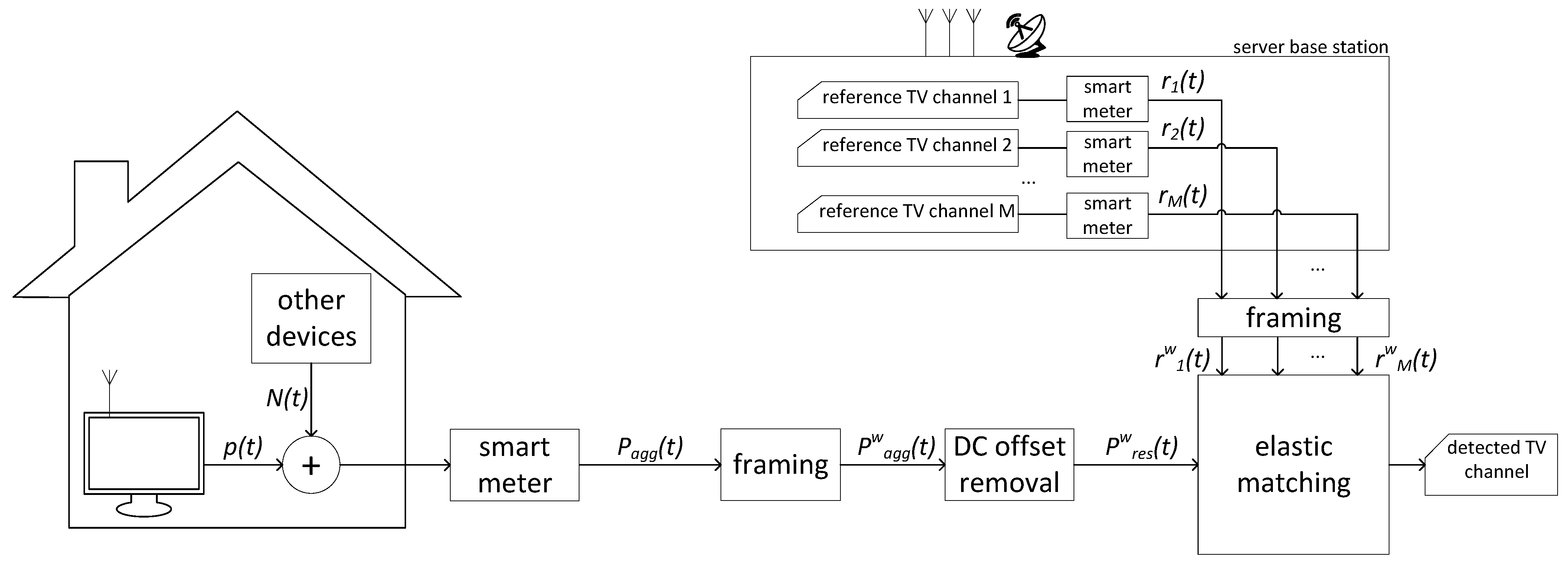
2. TV Channel Watching Identification from Smart Meter Data Architecture

The presented architecture aims to investigate the potential of identifying the TV channel watching preferences of residents based on the aggregated energy consumption signal measured by a smart meter at the main inlet of the household. The conceptual diagram of the architecture for the identification of watched TV channels using smart meter’s energy data is explicitly illustrated in Figure 1.

Specifically, the architecture in Figure 1 underlies the following five assumptions:

• The number of TV channels is of medium size (∼20 different channels);
• The noise of the ‘other devices’ is generated through multiple different scenarios, each with different noise levels. In detail, to assure realistic noise levels, noise data were generated using the UK-DALE dataset, which consists of real households energy measurements with a high number of appliances working in parallel;
• There is no time-lag between the recordings in the household and the server base station;
• In the considered household, a maximum of one TV device is turned on at the same time;
• The TV operates in real-time watching mode not in video on demand mode.

As can be seen in Figure 1, a smart meter measures the aggregated energy consumption, $P_{agg}\left(t\right)$, of a household. The aggregated signal is the sum of the energy consumption of all the devices of the house and in the present setup we consider the TV device (or a monitor) as the target device with energy consumption $p\left(t\right)$ and all other home appliances having energy consumption $N\left(t\right)$, meaning:

$$P_{agg}\left(t\right)=p\left(t\right)+N\left(t\right)=p\left(t\right)+\sum _{i=1}^{N-1}{n}_i\left(t\right)$$

(1)

where N is the number of all appliances of the household, including the TV device, fridge and washing machine, operating in the considered household.

Subsequently, the aggregated signal, $P_{agg}\left(t\right)$, is frame blocked in frames of constant length equal to W samples and from every energy frame, $P_{agg}^w\left(t\right)\in {\mathbb{R}}^w:P_{agg}(t-W:t)$, the DC offset is removed, resulting in $P_{res}^w$. The DC offset is removed due to the fact that most common home appliances like fridges, refrigerators, boilers, electric heating bodies, electric ovens etc., have energy consumption values within a range of 200–2000 Watts while the average energy consumption of a TV device or monitor is in the order of 25–250 Watts. Therefore, the DC part of the energy signal within each frame is attributed to devices with high energy consumption and after removing the remaining residual signal, $P_{res}^w\left(t\right)\in {\mathbb{R}}^W$, the contour shape characteristics of the energy signal of devices with lower energy consumption like the TV device will be shown more clearly.

Apart from the household aggregated energy consumption measurements, we considered a server base station where the broadband signals from M TV channels are received, assuming that M are all available TV channels. Each of the received signals is played by M reference TV devices of the same brand and model and the corresponding energy consumption signals, $r_m\left(t\right)$, with $1\le m\le M$, are measured by smart meters. It is worth mentioning that the TV devices used at the server base station are not the same with the TV device of the household. Then, each of the M reference signals, $r_m\left(t\right)$, is frame blocked in frames of constant length equal to W samples, i.e., $r_m^w\left(t\right)\in {\mathbb{R}}^W$.

Assuming there is no significant time-lag for the reception of the TV broadband signal between the house and the server base station, template matching (elastic matching) is performed between the unknown residual signal, $P_{res}^w\left(t\right)$, and each of the M reference signals, $r_m\left(t\right)$, the reference TV channel energy consumption signal with the lowest distance from the residual household’s signal, is considered as the detected TV channel $Ch\left(t\right)$ watched at time frame t, meaning:

$$Ch\left(t\right)=\underset{1\le m\le M}{arg\; min}\left\{f(P_{res}^w\left(t\right),r_m\left(t\right))\right\}$$

(2)

where $f(·)$ is a template (elastic) matching algorithm and $Ch\left(t\right)\in [1,...,M]$ is the detected TV channel watched at time frame t.

In order to provide more distinctive information, the above described architecture can be expanded with the elastic matching algorithm $f(·)$ not only considering the aggregated active power samples, but a set of F features $X_{res}^w\left(t\right)\in {\mathbb{R}}^{FxW}$ and $r_m^{{}^{\prime }}\left(t\right)\in {\mathbb{R}}^{FxW}$. The F features are computed from the raw current and voltage samples, $i_{agg}\left(t\right)$ and $v_{agg}\left(t\right)$, providing a set of the most common electrical features, e.g., reactive power or harmonics, and include the active power samples. Therefore, Equation (3) can be rewritten as

$$Ch\left(t\right)=\underset{1\le m\le M}{arg\; min}\left\{f(X_{res}^w\left(t\right),r_m^{{}^{\prime }}\left(t\right))\right\}$$

(3)

In the presented architecture, the case of not watching TV can be considered either by applying threshold values to the elastic matching algorithms of the detected TV channels or by considering not watching TV as an additional class, i.e., the (M + 1)th one. In addition, the architecture can be expanded to the case of more than two TV devices to play different channels simultaneously by considering one of them as belonging to the ‘other devices’ or by selecting all elastic matching scores below a threshold as detected devices. Furthermore, switching TV channels would not require a different architecture as the proposed methodology is performing TV channel identification at the frame level, thus only the frames capturing the switch time event would contain samples from two different TV channels, which will practically not affect the detected time period per channel by more than 1 frame (20 milliseconds), given that a user will watch a TV channel for at least few seconds before switching to another one.

3. Experimental Setup

The video classification architecture presented in Section 2 was evaluated using the dataset, energy features, classification models and experimental protocols presented below.

3.1. Evaluation Data

As there is no benchmark dataset with energy consumption measurements from the TV or monitoring devices, we recorded a dataset for video classification using the publicly available video footage from the THUMOS challenge 2014 [41]. In detail, we selected the first 26 videos from the background data, excluding videos 11, 14, 20, 23, 24 and 25, as their duration was less than 1 min, resulting in a set of 20 videos. Energy consumption data measurements were taken from two different monitors, namely an Acer P235H which was used as the test screen at the house as shown in Figure 1 and an Iiyama Prolite B2483HS which was used as a reference pattern at the servers station. The technical characteristics of the two monitors are tabulated in

Table 1. Technical characteristics of the monitors used.

	Acer P235H	Iiyama B2483HS
Technology	LCD	LED
Screen size (inch)	23	24
Brightness (cd/${\mathrm{m}}^2$)	300	250
Resolution (pixels)	1920 × 1080	1920 × 1080
Power (Watts)	31.7	24.9

.

For measuring the electrical energy consumption of the monitors, a hardware prototype smart meter developed by MEAZON (https://meazon.com/, accessed on 20 April 2021) was used for the first 1 min of each video. The smart meter is a energy circuit-level meter, measuring current, voltage, line frequency, active and reactive power and energy as well as harmonics and crest factor. It was designed for monitoring loads in an electrical board in commercial or industrial buildings or homes with an internal control capability up to 16 Amperes that can be extended further by driving an external relay. The USB port and the ARM Cortex M3 CPU run at 32 MHz Clock Speed with 512 Kbyte of In-System Programmable Flash and 32 Kbytes of Memory. All the above parameters, e.g., the active power or reactive power, were outputted once per electrical cycle by the smart meter, thus at a rate of 50 times per second. Specifically, the internal sampling rate for calculating each feature was 8000 Hz, thus for each output sample, 160 samples were used for the calculation. The prototype of the used smart meter is shown in Figure 2.

As regards the UK-DALE database [42], it was used to generate the energy consumption signal of N-1 ‘other devices’ from a real house. In particular, UK-DALE was chosen among other online available databases, e.g., REDD [43], ECO [44] or AMPds [45], since it provides high frequency measurements (16 kHz) of households combined with a large number of appliances operating in parallel. Specifically, we used one hour of the first house of UK-DALE (maximum of 52 appliances) from the 2 December 2014 between 4 p.m. and 5 p.m. due to the presence of between 1 and 26 electrical appliances within this time window, with none of them being a TV device. The aggregated current $i_{agg}\left(t\right)$ and the aggregated voltage $v_{agg}\left(t\right)$ were used to calculate the 19 features described in Section 3.2, e.g., $p_{agg}=\frac{1}{T_s}{\int }_0^{T_s}{v}_{agg}\left(t\right)·i_{agg}\left(t\right)dt$ in case of the active power. The calculated features were then utilized to generate the noise vector $N\left(t\right)$ as described in Section 2. In order to have the same sampling rate as measured by the smart meter, the data were down-sampled to 50 Hz.

3.2. Feature Extraction and Feature Ranking

The raw samples of the aggregated current and voltage, $i_{agg}$ and $v_{agg}$, was frame-blocked in frames of 160 samples. For every frame, a feature vector was calculated consisting of four statistical features (peak voltage ($\widehat{V}$), rms current/voltage (iFRMS, vFRMS), crest factor of current (cF)) and 15 electrical features (current (I), voltage (V), active power (P), frequency (f), reactive power (Q), apparent power (S), load angle ($\phi$), total harmonic distortion current/voltage (iTHD, vTHD), $3\mathrm{rd}$/$5\mathrm{th}$/$7\mathrm{th}$ harmonic current/voltage (iHD3/5/7, vHD3/5/7) resulting in the feature vectors of dimensionality equal to $F=19$. In order to calculate the statistical importance of the 19 features, the ReliefF feature ranking algorithm [46] was used by averaging the ranking scores across the 20 measured video signals. The results are illustrated in Figure 3.

As can be seen in Figure 3, in general, most of the electrical features outperform the statistical features with the most dominant features being the frequency, apparent power, raw current as well as of the set current and voltage harmonics. This is in line with previous publications reporting the high importance of electrical features [47,48]. Regarding the current and voltage harmonics, they carry a significant amount of the video playing energy signal’s information, e.g., both iHD5 and iHD7 have high feature ranking scores. Active power P, reactive power Q and apparent power S carry similar information as they can be computed by the relation $S=\sqrt{P^2+Q^2}$, thus Q has a relatively low feature ranking score as it can be computed by S and P. Especially, the results in Figure 3 illustrate that several different features contribute to an accurate description of the TV channels and thus using a single feature, e.g., current or voltage, might not be sufficient for identifying TV channels. Since it is not clear how discriminative electric measurements of monitors are when being used for TV channel classification, e.g., electrical measurements might be filtered through a large capacitor at the monitor input, and the time domain signals of eight different features are illustrated for two different video sequences in Figure 4.

As illustrated in Figure 4 all eight features show different shapes for the two different video signals, respectively. Specifically, the following four instances marked with bounding boxes (i)–(iv) were analysed. The first case, denoted as ‘(i)’, illustrates the voltage envelop over time for both videos showing a significantly stronger decrease in the red curve compared to the blue curve. The second case, denoted as ‘(ii)’, illustrates the difference between the two signals for the active power consumption. In detail, the time envelop of the signals was inversed, showing a decrease in the blue signal and an increase in the red signal. The third case, denoted as ‘(iii)’, illustrates the envelop of the THD of the voltage showing a significant peak for the blue signal while the red signal is relatively constant. The last case ‘(iv)’ shows the time envelop of the $7\mathrm{th}$ voltage harmonic, with the red signal being relatively constant while the blue signal has a significant drought. To summarize, Figure 4 illustrates that especially features with high feature ranking show significantly different patterns in the time domain for two different videos.

Further to feature ranking measurements, examples of the monitor’s energy consumption information carried by the active power, raw current and the $7\mathrm{th}$ current harmonic are illustrated in Figure 5, Figure 6 and Figure 7, respectively, including the aggregated signals before and after the frame’s DC offset removal.

3.3. Elastic Matching Algorithms

For the classification, four different well known and widely used elastic matching algorithms were employed, namely the dynamic time warping (DTW), soft dynamic time warping (sDTW), minimum variance matching (MVM), and global alignment kernel (GAK) [49,50,51]. Each of these algorithms can be used to compare one- and multi-dimensional time series’ of possible unequal length and thus found application in several areas of signal processing, e.g., speech processing [52,53], image processing [54,55] or energy disaggregation [16,56]. Each of these algorithms has advantages and disadvantages which make them appropriate or not for application in different problems. In detail, DTW is the oldest elastic matching algorithm and many modifications of it have been proposed for feature concatenation, e.g., parallel, serial and decoupled concatenation as described in [57], or restrictions on the warping path [58,59], improving the performance or the computational effort. However, DTW has the disadvantage of not having additional degrees of freedom in the warping path as offered by sDTW, GAK or MVM. Specifically, the sDTW and GAK allow a smoothing of the warping path and thus consider a richer presentation of the similarities of the two signals. This property was especially utilized for multi-step ahead prediction of time series’ [49,60], where the uncertainty between the elastic matching dataset and the example signatures increased with an increasing number of ahead predictions. Moreover, MVM gives an additional degree of freedom, namely allowing to skip outliers and matching sub-sequences without necessarily matching the first and last samples of the two sequences, conversely to DTW alignment where the first and last sample always have to be aligned. This property has been reported to be advantageous in several applications, i.e., in energy disaggregation scenarios with high noise levels or a small amount of training data [16]. The mathematical descriptions of these four template matching algorithms are presented below.

Let us consider the aggregated power consumption signal $P_{agg}\left(t\right)\forall t:t\in \{1,\cdots ,T\}$ as measured by a smart meter. For simplicity, let the $w\mathrm{th}$ frame of $P_{res}^w$ be denoted by $P_a$, where $P_a=[p\left(i\right),p(i+1),\cdots ,p(i+K)]$ be a sequence of length K where $p\left(i\right)$ is the $i\mathrm{th}$ sample of $P_{agg}$. Furthermore, let $P_b=[p\left(j\right),p(j+1),\cdots ,p(j+L)]$ be a second sequence of length L where $p\left(j\right)$ is the $j\mathrm{th}$ sample of $P_{agg}$ and $K<L$. Furthermore, let $\Delta (P_a,P_b)={\left[\delta (p_a^k,p_b^l)\right]}_{i,j}\in {\mathbb{R}}^{KxL}$ be an arbitrary cost matrix, where $\delta (·)$ is a distance metric, e.g., Euclidean distance, Manhattan distance or Kullback–Leibler (KL) distance and $\langle A,\Delta (P_a,P_b)\rangle$ being the inner product of matrix A with the cost matrix $\Delta (P_a,P_b)$, where A is an alignment matrix with $A_{k,l}$ giving the scores of A. Based on the above, the generalized $mi{n}^{\gamma }$ operator, with the smoothing parameter $\gamma \ge 0$, can be written as in Equation (4) and is referred to as soft dynamic time warping $dt{w}_{\gamma }$:

$$dt{w}_{\gamma }:=mi{n}^{\gamma }\{\langle A,\Delta (P_a,P_b)\rangle A\in A_{k,l}\}$$

(4)

$$mi{n}^{\gamma }\{a_1,\cdots ,a_k\}:=\left\{\begin{array}{cc}mi{n}_{i\le k}{a}_i\hfill & \gamma =0\hfill \\ -\gamma log\sum _{i=1}^k{e}^{-a_i/\gamma }\hfill & \gamma >0\hfill \end{array}\right.$$

(5)

where the original DTW score is recovered by setting $\gamma =0$. Extending the previous definition of sDTW, the Global Alignment (GA) kernel was defined as the exponentiated soft-minimum of all alignments distances and can be written as in Equation (6):

$$k_{GA}^{\gamma }:=\sum _{A\in A_{k,l}}{e}^{-\langle A,\Delta (P_a,P_b)\rangle /\gamma }$$

(6)

where $\gamma >0$ is the smoothing parameter of the kernel. Compared to DTW, $k_{GA}^{\gamma }$ incorporates the whole spectrum of costs $\langle A,\Delta (P_a,P_b)\rangle$ and thus provides a richer representation than the absolute minimum of set A, as considered by DTW.

In contrast to DTW, sDTW and GAK, MVM tries not to find the optimal alignment between the two sequences $P_a$ and $P_b$, but also considers the alignment of sub-sequences. Therefore, MVM tries to find a subsequence $P_a^{{}^{\prime }}$ of length K such that $P_b$ best matches $P_a^{{}^{\prime }}$. To formally describe MVM, the difference matrix r between the two sequences $P_a$ and $P_b$ and is defined as follows:

$$r=\left(r_{kl}\right)=(p_a^k-p_b^l)$$

(7)

Furthermore, $r_{kl}$ is treated as a directed graph with the following links [51]:

$$r_{kl}\leftrightarrow r_{rs}withr-k=1andl+1\le l+K-L$$

(8)

Using Equations (7) and (8) the least-value path in terms of the linkcost and pathcost can be written as described in [51].

A bootstrap training subset utilizing 50% of the evaluation data was used in order to optimize the free parameters of the elastic matching algorithms. The grid search results are shown in

Table 2. Classification accuracy (%) for different parameter values of the sDTW, GAK and MVM algorithms. Best performing parameter setups are marked with bold.

sDTW
$\mathit{\gamma }$	1	2	5	10	100	500
	91.0%	91.1%	91.3%	90.1%	89.8%	89.8%
GAK
$\mathit{\gamma }$	1	2	5	10	100	500
	52.3%	65.9%	71.8%	71.4%	69.7%	63.2%
MVM
v	5	10	15	20	25	30
	95.5%	95.6%	95.5%	95.5%	95.5%	95.5%

and the best elastic matching classification accuracy corresponding to the optimal values of each elastic matching algorithm are shown in bold.

As can be seen in Table 2, the optimal parameters of the elastic matching algorithms used are $\gamma =5$ for sDTW, $\gamma =5$ for GAK and $v=10$ for MVM. The best classification accuracy on the bootstrap training data was achieved by the MVM algorithm and was equal to 95.6%—outperforming all other evaluated elastic matching algorithms.

3.4. Experimental Protocols

To evaluate the proposed architecture, three different experimental protocols were utilized:

(A) Evaluation under noiseless conditions, i.e., $N\left(t\right)=0$, was carried out to determine whether or not different videos can be distinguished from their electrical energy signals recorded from the same monitors, thus in this protocol it will be $P\left(t\right)=P^{{}^{\prime }}\left(t\right)$. No DC offset removal was applied in this protocol as there were no other devices distorting the TV signal;

(B): Evaluation with additional ‘other devices’ was carried out, thus $N\left(t\right)={\sum }_{i=1}^{N-1}{n}_i\left(t\right)$, using the aggregated energy signal from the UK-DALE dataset and reference patterns from the same monitor, i.e., $P\left(t\right)=P^{{}^{\prime }}\left(t\right)$;

(C): Evaluation with additional ‘other devices’ was carried out using different monitors, i.e., $P\left(t\right)\ne P^{{}^{\prime }}\left(t\right)$, using Acer P235H monitor at the target house and Iiyama B2483HS monitor at server station.

For the additional ‘other devices’, 59 different sets of recordings were randomly selected from the 1 h duration measurements of the UK-DALE dataset and added to the energy measurement of the respective video signal. It must be noted that 59 noise scenarios were chosen in order to avoid zero padding for the $60\mathrm{th}$ noise scenario, as the 1 h UK-DALE datafile is slightly shorter than 60 min. Furthermore, it must be pointed out that the UK-DALE dataset consists of energy data measured from real households, thus providing a realistic noise scenario for the evaluations.

4. Experimental Results

The architecture presented in Section 2 for the identification of the TV channels watched using an outdoors smart meter was evaluated according to the experimental setup described in Section 3. The performance of the three evaluated protocols was estimated in terms of accuracy (ACC) and in terms of F-score ($F_1$), meaning:

$$ACC=\frac{TP+TN}{TP+TN+FP+FN}$$

(9)

$$F_1=\frac{2·TP}{2·TP+FN+FP}$$

(10)

where TP are the true positives, TN are the true negatives, FP are the false positives and FN are the false negatives, respectively. For each of the three experimental protocols (A, B and C) 21 energy signals (from playing 20 videos and one experiment with no video played) were tested for 60 different noise scenarios and the averaged results are tabulated in

Table 3. Classification results (%) for three experimental protocols (A) noiseless; (B) noisy; and (C) noisy using different monitors, averaged over 60 different noise scenarios. Best performing setups are marked with bold.

Classifier	ACC			F1
	A	B	C	A	B	C
DTW	100.0	82.6	81.1	100.0	81.6	80.2
sDTW	100.0	89.3	87.1	100.0	88.4	86.0
GAK	100.0	67.2	63.7	100.0	66.4	62.8
MVM	100.0	94.7	93.8	100.0	94.3	93.3

in terms of ACC and $F_1$ scores for the noiseless (A), noisy (B) and noisy using different monitors (C) experimental protocol.

As can be seen in Table 3, all four elastic matching algorithms were able to identify the played videos with 100% accuracy when intrusive load monitoring was used (protocol A) in a noiseless scenario. When identification was performed using the aggregated signal (protocol B) and using the same monitor (Acer P235H), MVM outperformed all other elastic matching algorithms, achieving an accuracy of 94.7% and an $F_1$ score 94.3%. In protocol C, elastic matching was performed on the signals from different monitors and MVM again achieved the highest performance among all evaluated algorithms (accuracy 93.8% and $F_1$ score 93.3%), which is in agreement with our previous study [16], where MVM was also found to perform well on the NILM task.

In a further step, the results of the best performing architecture (MVM) were evaluated using confusion matrices for the 21 signals and compared to the baseline system when utilizing DTW. First, when considering protocol A, there was no difference in terms of classification between DTW and MVM as all signals were perfectly classified for each of the 59 noise scenarios (Figure 8a,b). Second, for protocol B, there is a significant drop in performance for DTW, which is mostly due to the misclassification of TV signals with the case of not watching TV (Figure 8c,d). In detail, there were 35 misclassifications when utilizing DTW, while there were only five misclassifications when utilizing MVM. Third, in protocol C, a similar behaviour was observed as in protocol B with a high number of misclassifications and thus a relatively large performance decrease for DTW and only a small performance decrease for MVM (Figure 8e,f). In detail, there were 81 misclassifications with the scenario of not watching TV when utilizing DTW as elastic matching algorithm and 20 misclassifications for MVM, respectively. The results of protocols B and C are in line with the work presented in [61], where significantly better performances for elastic matching were reported in noisy scenarios when utilizing MVM. Furthermore, a similar behaviour was reported in our previous study where MVM has also been proven to enhance accuracy for the energy disaggregation task [16].

5. Conclusions

Currently, TV audience measurements are made by companies that have installed monitoring devices in a limited number of households, e.g., BARB in the UK. Identifying TV channel watching from the household’s smart meter expands the usage of the device beyond energy monitoring and allows energy supplier companies to also offer other commercial services. On the other hand, the detection of multimedia content from smart meters raises concerns regarding the privacy of households. In this paper, we investigated the potential of identifying the watched TV channel or multimedia content using a smart meter installed outside a house by comparing the household’s aggregated energy consumption signal with a closed set of reference signals acquired from the energy consumption of other monitor devices. The experimental results for a set of 20 possible TV channel options revealed that this is possible and the best identification performance, achieved by the MVM elastic matching algorithm, was equal to 93.8% in terms of accuracy and 93.3% in terms of $F_1$ score, followed by sDTW reporting performances of 87.1% in terms of accuracy and 86.0% in terms of $F_1$ score. Conversely, DTW has reported slightly worse results, while GAK was not able to match the performance of the other algorithms. It was also shown that all of the investigated elastic matching algorithms were capable of dealing with different noise levels, as well as with different monitors installed at the server station and the local TV under investigation, which is crucial for a real world implementation. Moreover, it was shown that elastic matching algorithms are a suitable choice for identifying TV channels in real-time as they do not rely on training a classifier and thus can be used directly without previous training and can operate continuously without need for the re-training of any models. The proposed proof of concept methodology was evaluated under a number of assumptions and in a next research direction, will be tested considering a large scale experimental setup including several houses with different locations and varying time-lags between the server broadcasting station and the receivers which can be addressed by expanding the elastic matching search to the previous N-frames as well as different types of TV devices, including smart TVs. Finally, the effect of multiple TVs operating simultaneously in a household should be investigated.

References

1. Cooper, A. Electric Company Smart Meter Deployments: Foundation for a Smart Grid; The Institute for Electric Innovation (IEI): Washington, DC, USA, 2016. [Google Scholar]
2. Zhou, S.; Brown, M.A. Smart meter deployment in Europe: A comparative case study on the impacts of national policy schemes. J. Clean. Prod. 2017, 144, 22–32. [Google Scholar] [CrossRef]
3. Althaher, S.; Mancarella, P.; Mutale, J. Automated demand response from home energy management system under dynamic pricing and power and comfort constraints. IEEE Trans. Smart Grid 2015, 6, 1874–1883. [Google Scholar] [CrossRef]
4. Hart, G.W. Nonintrusive appliance load monitoring. Proc. IEEE 1992, 80, 1870–1891. [Google Scholar] [CrossRef]
5. Figueiredo, M.; Ribeiro, B.; de Almeida, A. Electrical Signal Source Separation Via Nonnegative Tensor Factorization Using On Site Measurements in a Smart Home. IEEE Trans. Instrum. Meas. 2014, 63, 364–373. [Google Scholar] [CrossRef]
6. Rahimpour, A.; Qi, H.; Fugate, D.; Kuruganti, T. Non-Intrusive Energy Disaggregation Using Non-Negative Matrix Factorization with Sum-to-k Constraint. IEEE Trans. Power Syst. 2017, 32, 4430–4441. [Google Scholar] [CrossRef]
7. Makonin, S.; Bajic, I.V.; Popowich, F. Efficient Sparse Matrix Processing for Nonintrusive Load Monitoring (NILM). Available online: http://nilmworkshop.org/2014/proceedings/makonin_efficient.pdf (accessed on 8 March 2021).
8. Schirmer, P.A.; Mporas, I.; Sheikh-Akbari, A. Energy Disaggregation Using Two-Stage Fusion of Binary Device Detectors. Energies 2020, 13, 2148. [Google Scholar] [CrossRef]
9. Johnson, M.J.; Willsky, A.S. Bayesian nonparametric hidden semi-Markov models. J. Mach. Learn. Res. 2013, 14, 673–701. [Google Scholar]
10. He, K.; Jakovetic, D.; Zhao, B.; Stankovic, V.; Stankovic, L.; Cheng, S. A Generic Optimisation-Based Approach for Improving Non-Intrusive Load Monitoring. IEEE Trans. Smart Grid 2019, 10, 6472–6480. [Google Scholar] [CrossRef] [Green Version]
11. Harell, A.; Makonin, S.; Bajić, I.V. Wavenilm: A Causal Neural Network for Power Disaggregation from the Complex Power Signal. Available online: https://ieeexplore.ieee.org/document/8682543 (accessed on 8 March 2021).
12. Schirmer, P.A.; Glose, D. Optimal Interleaved Modulation for DC- Link Loss Optimization in Six-Phase Drives. In Proceedings of the 2019 IEEE 13th International Conference on Power Electronics and Drive Systems (PEDS), Toulouse, France, 9–12 July 2019; pp. 1–6. [Google Scholar]
13. Schirmer, P.A.; Mporas, I.; Sheikh-Akbari, A. Robust energy disaggregation using appliance-specific temporal contextual information. EURASIP J. Adv. Signal Process. 2020, 2020, 394. [Google Scholar] [CrossRef] [Green Version]
14. Makonin, S. Investigating the switch continuity principle assumed in Non-Intrusive Load Monitoring (NILM). In Proceedings of the 2016 IEEE Canadian Conference on Electrical and Computer Engineering (CCECE), Vancouver, BC, Canada, 15–18 May 2016; IEEE: Piscataway, NJ, USA, 2016; pp. 1–4. [Google Scholar]
15. Kaselimi, M.; Doulamis, N.; Doulamis, A.; Voulodimos, A.; Protopapadakis, E. Bayesian-optimized Bidirectional LSTM Regression Model for Non-intrusive Load Monitoring. In Proceedings of the ICASSP 2019—2019 IEEE International Conference on Acoustics, Speech and Signal Processing (ICASSP), Brighton, UK, 12–17 May 2019; pp. 2747–2751. [Google Scholar]
16. Schirmer, P.A.; Mporas, I.; Paraskevas, M. Energy Disaggregation Using Elastic Matching Algorithms. Entropy 2020, 22, 71. [Google Scholar] [CrossRef] [PubMed] [Green Version]
17. Liao, J.; Elafoudi, G.; Stankovic, L.; Stankovic, V. Power Disaggregation for Low-sampling Rate Data. Available online: http://nilmworkshop.org/2014/proceedings/liao_power.pdf (accessed on 8 March 2021).
18. Lin, Y.H.; Tsai, M.S. An Advanced Home Energy Management System Facilitated by Nonintrusive Load Monitoring with Automated Multiobjective Power Scheduling. IEEE Trans. Smart Grid 2015, 6, 1839–1851. [Google Scholar] [CrossRef]
19. Kelly, J.; Knottenbelt, W. Does Disaggregated Electricity Feedback Reduce Domestic Electricity Consumption? A Systematic Review of the Literature. Available online: https://arxiv.org/pdf/1605.00962.pdf (accessed on 8 March 2021).
20. Ju, C.; Wang, P.; Goel, L.; Xu, Y. A two-layer energy management system for microgrids with hybrid energy storage considering degradation costs. IEEE Trans. Smart Grid 2017, 9, 6047–6057. [Google Scholar] [CrossRef]
21. Pilz, M.; Al-Fagih, L. A dynamic game approach for demand-side management: Scheduling energy storage with forecasting errors. Dyn. Games Appl. 2019, 10, 897–929. [Google Scholar] [CrossRef] [Green Version]
22. Shimizu, Y.; Sakagami, T.; Kitano, H. Prediction of weather dependent energy consumption of residential housings. In Proceedings of the 6th IEEE International Conference on Renewable Energy Research and Applications (ICRERA 2017), San Diego, CA, USA, 5–8 November 2017; IEEE: Piscataway, NJ, USA, 2017; pp. 967–970. [Google Scholar]
23. Schirmer, P.A.; Geiger, C.; Mporas, I. Residential energy consumption prediction using inter-household energy data and socioeconomic information. In Proceedings of the 2020 28th European signal processing conference (EUSIPCO), Amsterdam, The Netherlands, 24–28 August 2020; pp. 1595–1599. [Google Scholar]
24. Schirmer, P.A.; Geiger, C.; Mporas, I. Reducing Grid Distortions Utilizing Energy Demand Prediction and Local Storages. IEEE Access 2021, 9, 15122–15132. [Google Scholar] [CrossRef]
25. Zeifman, M. Disaggregation of home energy display data using probabilistic approach. IEEE Trans. Consum. Electron. 2012, 58, 23–31. [Google Scholar] [CrossRef]
26. Bousbiat, H.; Klemenjak, C.; Leitner, G.; Elmenreich, W. Augmenting an Assisted Living Lab with Non-Intrusive Load Monitoring. In Proceedings of the 2020 IEEE International Instrumentation and Measurement Technology Conference (I2MTC), Dubrovnik, Croatia, 25–28 May 2020; pp. 1–5. [Google Scholar]
27. Mrabet, Z.E.; Kaabouch, N.; Ghazi, H.E.; Ghazi, H.E. Cyber-security in smart grid: Survey and challenges. Comput. Electr. Eng. 2018, 67, 469–482. [Google Scholar] [CrossRef] [Green Version]
28. Anzalchi, A.; Sarwat, A. A survey on security assessment of metering infrastructure in smart grid systems. In Proceedings of the SoutheastCon 2015, Fort Lauderdale, FL, USA, 9–12 April 2015; pp. 1–4. [Google Scholar]
29. McLaughlin, S.; McDaniel, P.; Aiello, W. Protecting consumer privacy from electric load monitoring. In Proceedings of the 18th ACM Conference on Computer and Communications Security, Chicago, IL, USA, 17–21 October 2011; Chen, Y., Danezis, G., Shmatikov, V., Eds.; ACM: New York, NY, USA, 2011; p. 87. [Google Scholar]
30. Ur-Rehman, O.; Zivic, N.; Ruland, C. Security issues in smart metering systems. In Proceedings of the 2015 IEEE International Conference on Smart Energy Grid Engineering (SEGE), Oshawa, ON, Canada, 17–19 August 2015; pp. 1–7. [Google Scholar]
31. Zhao, J.; Liu, J.; Qin, Z.; Ren, K. Privacy protection scheme based on remote anonymous attestation for trusted smart meters. IEEE Trans. Smart Grid 2016, 9, 3313–3320. [Google Scholar] [CrossRef]
32. Dong, R.; Ratliff, L.J. Energy Disaggregation and the Utility-Privacy Tradeoff. In Big Data Application in Power Systems; Arghandeh, R., Zhou, Y., Eds.; Elsevier: Amsterdam, The Netherlands, 2017; pp. 409–444. [Google Scholar]
33. Li, D.; Bissyande, T.F.; Kubler, S.; Klein, J.; Le Traon, Y. Profiling household appliance electricity usage with N-gram language modeling. In Proceedings of the 2016 IEEE International Conference on Industrial Technology (ICIT), Taipei, Taiwan, 14–17 March 2016; IEEE: Piscataway, NJ, USA, 2016; pp. 604–609. [Google Scholar]
34. Papagiannakopoulou, E.I.; Koukovini, M.N.; Lioudakis, G.V.; Garcia-Alfaro, J.; Kaklamani, D.I.; Venieris, I.S.; Cuppens, F.; Cuppens-Boulahia, N. A privacy-aware access control model for distributed network monitoring. Comput. Electr. Eng. 2013, 39, 2263–2281. [Google Scholar] [CrossRef] [Green Version]
35. Wang, T.K.; Chang, F.R. Network time protocol based time-varying encryption system for smart grid meter. In Proceedings of the 2011 IEEE Ninth International Symposium on Parallel and Distributed Processing with Applications Workshops, Busan, Korea, 26–28 May 2011; pp. 99–104. [Google Scholar]
36. Greveler, U.; Glösekötterz, P.; Justusy, B.; Loehr, D. Multimedia content identification through smart meter power usage profiles. In Proceedings of the International Conference on Information and Knowledge Engineering (IKE), the Steering Committee of the World Congress in Computer Science, Computer, Las Vegas, NV, USA, 16–19 July 2012; p. 1. [Google Scholar]
37. Bouhouras, A.S.; Gkaidatzis, P.A.; Panagiotou, E.; Poulakis, N.; Christoforidis, G.C. A NILM algorithm with enhanced disaggregation scheme under harmonic current vectors. Energy Build. 2019, 183, 392–407. [Google Scholar] [CrossRef]
38. Gao, J.; Kara, E.C.; Giri, S.; Berges, M. A feasibility study of automated plug-load identification from high-frequency measurements. In Proceedings of the 2015 IEEE Global Conference on Signal and Information Processing (GlobalSIP), Orlando, FL, USA, 14–16 December 2015; IEEE: Piscataway, NJ, USA, 2015; pp. 220–224. [Google Scholar]
39. Schirmer, P.A.; Mporas, I. Energy Disaggregation Using Fractional Calculus. In Proceedings of the ICASSP 2020—2020 IEEE International Conference on Acoustics, Speech and Signal Processing (ICASSP), Barcelona, Spain, 4–8 May 2020; pp. 3257–3261. [Google Scholar] [CrossRef]
40. Schirmer, P.A.; Mporas, I. Energy Disaggregation from Low Sampling Frequency Measurements Using Multi-Layer Zero Crossing Rate. In Proceedings of the ICASSP 2020—2020 IEEE International Conference on Acoustics, Speech and Signal Processing (ICASSP), Barcelona, Spain, 4–8 May 2020; pp. 3777–3781. [Google Scholar] [CrossRef]
41. Jiang, Y.G.; Liu, J.; Zamir, A.R.; Toderici, G.; Laptev, I.; Shah, M.; Sukthankar, R. THUMOS Challenge: Action Recognition with a Large Number of Classes. Available online: http://crcv.ucf.edu/THUMOS14/ (accessed on 8 March 2021).
42. Kelly, J.; Knottenbelt, W. The UK-DALE dataset, domestic appliance-level electricity demand and whole-house demand from five UK homes. Sci. Data 2015, 2, 150007. [Google Scholar] [CrossRef] [PubMed] [Green Version]
43. Kolter, J.Z.; Johnson, M.J. (Eds.) REDD: A Public Data Set for Energy Disaggregation Research. Available online: https://people.csail.mit.edu/mattjj/papers/kddsust2011.pdf (accessed on 8 March 2021).
44. Beckel, C.; Kleiminger, W.; Cicchetti, R.; Staake, T.; Santini, S. The ECO data set and the performance of non-intrusive load monitoring algorithms. In BuildSys’14; Srivastava, M., Ed.; ACM: New York, NY, USA, 2014; pp. 80–89. [Google Scholar]
45. Makonin, S.; Popowich, F.; Bartram, L.; Gill, B.; Bajić, I.V. AMPds: A public dataset for load disaggregation and eco-feedback research. In Proceedings of the 2013 IEEE Electrical Power & Energy Conference, Vancouver, BC, Canada, 21–25 July 2013; pp. 1–6. [Google Scholar]
46. Urbanowicz, R.J.; Meeker, M.; LaCava, W.; Olson, R.S.; Moore, J.H. Relief-Based Feature Selection: Introduction and Review. J. Biomed. Informatics 2018, 85, 189–203. [Google Scholar] [CrossRef] [PubMed]
47. Ghorbanpour, S.; Mallipeddi, R. Significance of Classifier and Feature Selection in Automatic Identification of Electrical Appliances. In Proceedings of the 2018 IEEE International Conference on Systems, Man, and Cybernetics (SMC), Miyazaki, Japan, 7–8 October 2018; pp. 4184–4189. [Google Scholar]
48. Huang, N.; Wang, W.; Wang, S.; Wang, J.; Cai, G.; Zhang, L. Incorporating load fluctuation in feature importance profile clustering for day-ahead aggregated residential load forecasting. IEEE Access 2020, 8, 25198–25209. [Google Scholar] [CrossRef]
49. Cuturi, M.; Blondel, M. Soft-DTW: A Differentiable Loss Function for Time-Series. Available online: https://dl.acm.org/doi/10.5555/3305381.3305474 (accessed on 8 March 2021).
50. Cuturi, M. Fast Global Alignment Kernels. In Proceedings of the 28th International Conference on International Conference on Machine Learning (ICML’11), Bellevue, WA, USA, 28 June–2 July 2011; pp. 929–936. [Google Scholar]
51. Longin Jan Latecki, V.M.Q.W.D.Y. An elastic partial shape matching technique. Pattern Recognit. 2007, 40, 3069–3080. [Google Scholar] [CrossRef] [Green Version]
52. Juang, B.H. On the hidden Markov model and dynamic time warping for speech recognition—A unified view. AT&T Bell Lab. Tech. J. 1984, 63, 1213–1243. [Google Scholar]
53. Abdulla, W.H.; Chow, D.; Sin, G. Cross-words reference template for DTW-based speech recognition systems. In Proceedings of the TENCON 2003—Conference on Convergent Technologies for Asia-Pacific Region, Bangalore, India, 15–17 October 2003; Volume 4, pp. 1576–1579. [Google Scholar]
54. Cheng, H.; Dai, Z.; Liu, Z. Image-to-class dynamic time warping for 3D hand gesture recognition. In Proceedings of the 2013 IEEE International Conference on Multimedia and Expo (ICME), San Jose, CA, USA, 15–19 July 2013; pp. 1–6. [Google Scholar]
55. Sharma, S.K.; Phan, H.; Lee, J. An application study on road surface monitoring using DTW based image processing and ultrasonic sensors. Appl. Sci. 2020, 10, 4490. [Google Scholar] [CrossRef]
56. Liao, J.; Elafoudi, G.; Stankovic, L.; Stankovic, V. Non-intrusive appliance load monitoring using low-resolution smart meter data. In Proceedings of the 2014 IEEE International Conference on Smart Grid Communications (SmartGridComm 2014), Venice, Italy, 3–6 November 2014; IEEE: Piscataway, NJ, USA, 2014; pp. 535–540. [Google Scholar]
57. Liu, B.; Luan, W.; Yu, Y. Dynamic time warping based non-intrusive load transient identification. Appl. Energy 2017, 195, 634–645. [Google Scholar] [CrossRef]
58. Itakura, F. Minimum prediction residual principle applied to speech recognition. IEEE Trans. Acoust. Speech Signal Process. 1975, 23, 67–72. [Google Scholar] [CrossRef]
59. Sakoe, H.; Chiba, S. Dynamic programming algorithm optimization for spoken word recognition. IEEE Trans. Acoust. Speech Signal Process. 1978, 26, 43–49. [Google Scholar] [CrossRef] [Green Version]
60. Cuturi, M.; Vert, J.P.; Birkenes, O.; Matsui, T. A kernel for time series based on global alignments. In Proceedings of the 2007 IEEE International Conference on Acoustics, Speech and Signal Processing—ICASSP’07, Honolulu, HI, USA, 15–20 April 2007; Volume 2, pp. II–413–II–416. [Google Scholar]
61. Latecki, L.J.; Megalooikonomou, V.; Wang, Q.; Lakaemper, R.; Ratanamahatana, C.A.; Keogh, E. Elastic Partial Matching of Time Series. In Knowledge Discovery in Databases; Jorge, A.M., Torgo, L., Brazdil, P., Camacho, R., Gama, J., Eds.; Springer: Berlin/Heidelberg, Germany, 2005; pp. 577–584. [Google Scholar]
Figure 1. Block diagram of the architecture for identifying the TV channel being watched using smart meter data.
Energies 14 02485 g001
Figure 2. Cerberus smart meter from MEAZON: (a) CAD drawing including PCB and casing (b) the smart meter device.
Energies 14 02485 g002
Figure 3. Feature ranking for the set of 4 statistical (red) and 15 electrical features (blue).
Energies 14 02485 g003
Figure 4. Illustration of eight different features for two different video sequences on the same monitor (blue: video #1, red: video #2). Specifically, the following four instances marked with bounding boxes (i)–(iv) show significant differences between the two video signals.
Energies 14 02485 g004
Figure 5. Illustration of the active power of (a) the TV/monitor only; (b) other appliances; (c) the aggregated signal; and (d) the aggregated signal after DC offset removal.
Energies 14 02485 g005
Figure 6. Illustration of the current of (a) the TV/monitor only; (b) other appliances; (c) the aggregated signal; and (d) the aggregated signal after DC offset removal.
Energies 14 02485 g006
Figure 7. Illustration of the 7 th current harmonic of (a) the TV/monitor only; (b) other appliances; (c) the aggregated signal; and (d) the aggregated signal after DC offset removal.
Energies 14 02485 g007
Figure 8. Confusion matrix for three different experimental protocols using DTW and MVM as elastic matching algorithms (for best visibility, the reader is referred to the electronic version of the document).
Energies 14 02485 g008