Understanding the Potential of Wind Farm Exploitation in Tropical Island Countries: A Case for Indonesia

Abstract

Countries worldwide must dramatically reduce their emissions to achieve the goal of limiting temperature increases in line with the Paris Agreement. Involving developing countries in global actions on emission reduction will greatly enhance the effectiveness of global warming mitigation. This study investigated the feasibility of establishing a wind farm at four onshore and three offshore sites in Indonesia. Installing wind turbines with the highest hub height, largest rotor diameter, and lowest cut-in and rated wind speed in an identified area off Wetar Island presented the highest time-based availability and a capacity factor of 46%, as well as the highest power-based availability at 76%. The levelized cost of electricity at 0.082 USD/kWh was comparable to that of power generated from fossil fuels, which ranges from 0.07 to 0.15 USD/kWh in Indonesia. Increasing the feed-in-tariff for wind power from the current 0.08 USD/kWh would provide sufficient incentive for investment. Moving subsidies from fossil fuels toward renewables would facilitate the transition to low-carbon renewables without increasing the financial burden on the country.

1. Introduction

With climatic catastrophes, such as floods and wildfires occurring worldwide, the United Nations Environmental Programme announced that dramatic strengthening of nationally determined contributions (NDCs) to emission cuts is required in 2020. Countries must increase their NDC ambitions threefold to achieve the “well below 2 °C goal” and more than fivefold to achieve the 1.5 °C goal. To be in line with the Paris Agreement, emissions must drop 7.6% per year from 2020 to 2030 to reach the 1.5 °C goal and 2.7% per year to reach the 2 °C goal. Greater cuts will be required the longer action is delayed [1]. These alarming estimates indicate that more active emission cuts are required worldwide. However, energy demand and fossil fuel use are expected to grow in the coming decades due to population and economic growth in many developing countries [2]. Promoting the use of renewable energy in these countries is essential to the global effort to mitigate global warming.

A part of the global trend in energy transition, the Association of Southeast Asian Nations (ASEAN) is devoted to the development of renewable energy in this region. It set a target of renewable energy comprising 23% of total primary energy supply by 2025, compared with 9.4% in 2014. However, current policies are projected to reach only a renewable energy share of 17% by 2025, creating a 6% “gap” [3].

Indonesia is the most populated country in ASEAN and the largest archipelago country in the world, with more than 17,000 islands. Many remote islands are untouched by the national electricity grid. The development of renewable energy is especially crucial to meet the energy needs of these islands. Micro hydroelectric power systems are a possible renewable energy source for more remote islands because they are simple and affordable. Wind and photovoltaic energy sources offer solutions on islands with few water sources. According to the Indonesian Ministry of Energy and Mineral Resources, the national target for renewable energy is a share of 23% by 2025 and 31% by 2050 [4]. Developing renewable energy on remote islands is necessary to reach this goal.

Indonesia is a tropical country located near the equator. Sunlight produces a nearly uniform temperature throughout the year with little wind variation. The region where this phenomenon occurs, known as the doldrums and the Intertropical Convergence Zone, is located only near the equator. In the doldrums, the prevailing trade winds of the northern hemisphere blow to the southwest and collide with the southern hemisphere’s northeast trade winds. The winds blow up into the atmosphere and return to the northern and southern hemispheres, and velocity distribution near the equator becomes low to marginal. The doldrums are typically located within the five-degree latitude of the equator [5].

Wind energy utilization in Indonesia was recently realized with the establishment of the first wind farm, Sidrap Wind Farm, located on South Sulawesi Island. Hardianto et al. indicated that the potential of wind power at a height of 43.2 m reaches 277.03 W/m² in Puger Beach, East Java [6]. Martosaputro and Murti performed a preliminary analysis to investigate wind energy potential for Indonesia. It showed that wind energy resources are available on the south coast of Java Island, the eastern part of Indonesia, and the south part of Sulawesi Island [7]. Some parts of Sumantera, Kalimantan, and Papua, especially the islands, also have resources for wind energy that can be utilized to generate electricity, especially in rural and remote areas where access to electricity facilities remains limited.

The development of and investment in wind farms depend on accurate wind resource evaluation, which requires reliable wind measurement data and appropriate methodologies. One of the most widely used models for evaluating onshore and offshore wind resources is the Weather Research and Forecasting (WRF) model [8,9,10]. This mesoscale model enables the application of various numerical and physical options to a set of atmospheric and geographic scales [11,12]. These capabilities of the WRF model enable the simulation of wind fields worldwide [8,13], making it a useful tool for conducting wind prospecting studies where meteorological data are unavailable.

The performance of the WRF model has been examined in numerous studies. Olaofe [14] analyzed the spatial distributions of historical wind conditions by using the WRF model to quantify long-term changes in surface wind conditions off the African coast. These long-term historical wind conditions in time and space revealed that the WRF model is a reliable tool for replicating the coastal wind conditions of Africa. Salvaçáo and Guedes Soares [15] simulated a 10-year wind hindcast for the Iberian Peninsula coast with the WRF model at a spatial resolution of 9 and 3 km and a 6-hourly output. The amount of energy that can be generated by an energy conversion device, as well as the annual operating hours and capacity factors, were estimated and presented as wind resource maps. Comparisons with observational data revealed that the WRF model is a proficient tool for use in wind-power generation surveys in both coastal waters and the open ocean, and even when the model is run at a low spatial resolution. Prósper et al. [16] conducted a production forecast and validation study for a real onshore wind farm in a complex region with abundant wind resources in Galicia, northwestern Spain, by using WRF model simulations with high horizontal and vertical resolution. The results revealed that the WRF model yields favorable wind power operational predictions for the wind farms.

In addition to the necessity of using a sophisticated tool for evaluating wind resources, the layout of a wind farm affects the efficacy of its power generation. The optimization of a wind farm layout involves identifying the optimal locations for wind turbines in a wind farm to maximize the total energy output of the farm. Bansal and Farswan [17] used a biogeography-based approach to optimize wind farm layout by maximizing energy production and reducing the wake effect. Patel et al. [18] used a geometric pattern-based approach to optimize wind farm layout by maximizing the total power output of a wind farm. Park and Law [19] employed a mathematical optimization scheme to efficiently optimize the locations of wind turbines for maximizing wind farm power production. Considering the emerging trend of replacing fossil fuels with renewable energy for mitigating climate change, maximizing wind farm power production has become a major element of wind farm optimization.

In this context, this study investigated the feasibility of establishing wind farms in four onshore (Banyuwangi, Baron, Lebak, and Sukabumi) and three offshore (Jeneponto, Wetar Island, and Banten) locations in Indonesia. The selection of these locations was based on a preliminary wind assessment for Indonesia [7]. The wind properties in these locations were characterized to select the most suitable site with the best wind speed distribution and power production estimation. A wind farm design was then simulated and analyzed for each location to determine the optimal farm size and layout. Finally, an economic analysis was performed using discounted cash flow models to determine the most feasible investment scenario.

2. Methodology

2.1. Sites for Evaluation

The sites for evaluation in this study were onshore sites in Banyuwangi, Baron, Sukabumi, and Lebak in the south of Java Island, and offshore sites in Banten, Jeneponto, and Wetar Island (Figure 1).

2.2. Wind Dataset

WRF mesoscale maps were used as the wind data source for this study. Established in 2017 by EMB International A/S, Denmark, they are financed by the Environmental Support Programme (ESP3)/Daninda in collaboration with the Indonesian Ministry of Energy and Mineral Resources. The WRF dataset has a resolution of 0.029° (ca. 3 km) and is driven by ERA-Interim global data for the period 2004–2015 (Figure 1). The maps contain weather data for all of Indonesia. WRF data were used because of their relatively high spatial resolution as well as their availability and quality; actual high-quality wind data for Indonesia were unavailable. The measurement heights were 10, 25, 50, 75, 100, 150, and 200 m. WRF wind data at 1-h time intervals at heights of 100 m were used in this analysis in accordance with the hub height of modern wind turbines.

2.3. Wind Characteristics

Wind speed trends were identified using monthly averaged wind speeds from 2004 to 2015 to include speeds in rainy and dry seasons. Speeds at 100 m were then analyzed using a Weibull fit distribution estimation to determine annual wind speed distributions. The Weibull fit distribution parameters were compared to determine the wind speed characteristics of each site so that optimal potential sites could be identified.

The energy production of a wind turbine was calculated using wind speed and the turbine power curve. The energy production status of a wind turbine was classified as below the cut-in wind speed, between the cut-in and rated wind speed, the rated wind speed, and the cut-out wind speed as follows:

$$\begin{gathered} V_w<V_i, P_w=0 \\ {V}_i\le V_w<V_r, P_w=P_i \\ {V}_r\le V_w<V_o, P_w=P_r \\ {V}_o<V_w, P_w=0 \end{gathered}$$

where V_w is wind speed, V_i is cut-in wind speed, P_w is power output, V_r is rated wind speed, P_i is power output interpolated from the power curve, V_o is cut-out wind speed, and P_r is rated power output.

The analysis was performed using the wind data input into the turbine power curve, after which the power production was interpolated using the power curve. The annual total power production was then aggregated. Three types of wind turbines built by different manufacturers in the wind energy market were selected. The turbines are widely used by wind energy researchers for the middle wind speed region. The availability of power curves of wind turbines, which are often commercially confidential, was also considered. The technical specifications of the three commercial wind turbines selected for the study indicated that wind turbine C has the highest hub height, the largest rotor diameter, and the lowest cut-in and rated wind speed (

Table 1. Technical specifications of selected wind turbines.

Turbine	IEC Class	Rated Output (kW)	Hub Height (m)	Rotor Diameter (m)	Cut-In Wind Speed (m/s)	Rated Wind Speed (m/s)	Cut-Out Wind Speed (m/s)
A	IIIA	1800	90	100	4	12	20
B	IIB	2300	80	90	4	13	25
C	IIIA	2000	93	114	2	10	25

).

2.4. WindSim

WindSim is a wind farm design tool based on computational fluid dynamics and used to solve flow equations in body-fitted geometry. It employs a 3D Reynolds Averaged Navier–Stokes (RANS) solver and is appropriate for sites with complex climatology and terrain. The input data for the WindSim simulation was a terrain model that included information about terrain orography, roughness, and objects. Meteorological data from one or more sites inside the modeled area were also required. This study was aimed at identifying the best-case scenario for a wind farm on Wetar Island. Turbulence intensity was not discussed because it was not a priority of the study. The main work focused on using the outputs of WindSim (wind speed, wind direction, and turbulence intensity) to establish the wind turbine layout for each scenario and further determine which scenario was both technically and economically viable.

2.5. Wind Farm Performance

The effectiveness of the wind farms was evaluated for time-based availability, power production-based availability, and capacity factor. The capacity factor represents the amount of electricity produced relative to its turbine-rated power capacity. At times, the turbine stops operating due to low wind speed conditions or for maintenance. Time-based availability describes the effective operation time of the turbine, as represented below:

$$A_t=\frac{T_o}{T_t}\times 100\%$$

where A_t is time-based availability, T_o is turbine operating hours, and T_t is total hours in one year.

Power-based availability is the ratio of energy produced by a wind farm to expected power production. It can be expressed as follows:

$$A_p=\frac{E}{E_x}\times 100\%$$

where A_p is the power-based availability, E is the power production of the wind farm, and E_x is the expected power production of the wind farm calculated from the estimated power production of a single turbine using the WRF dataset multiplied by the number of turbines in the farm.

2.6. Economic Analysis of Wind Farm Design

An economic evaluation was performed to determine the investment value of the wind farm and the feasibility of the project. In this study, the wind farm cost model was derived from Cali et al. [21], who split the model into capital expenditures (CapEx) and operational expenditures (OpEx). An investment indicator was also included in the investment scenario. Wind farm scenarios were obtained from WindSim results.

3. Wind Characteristics of the Studied Sites

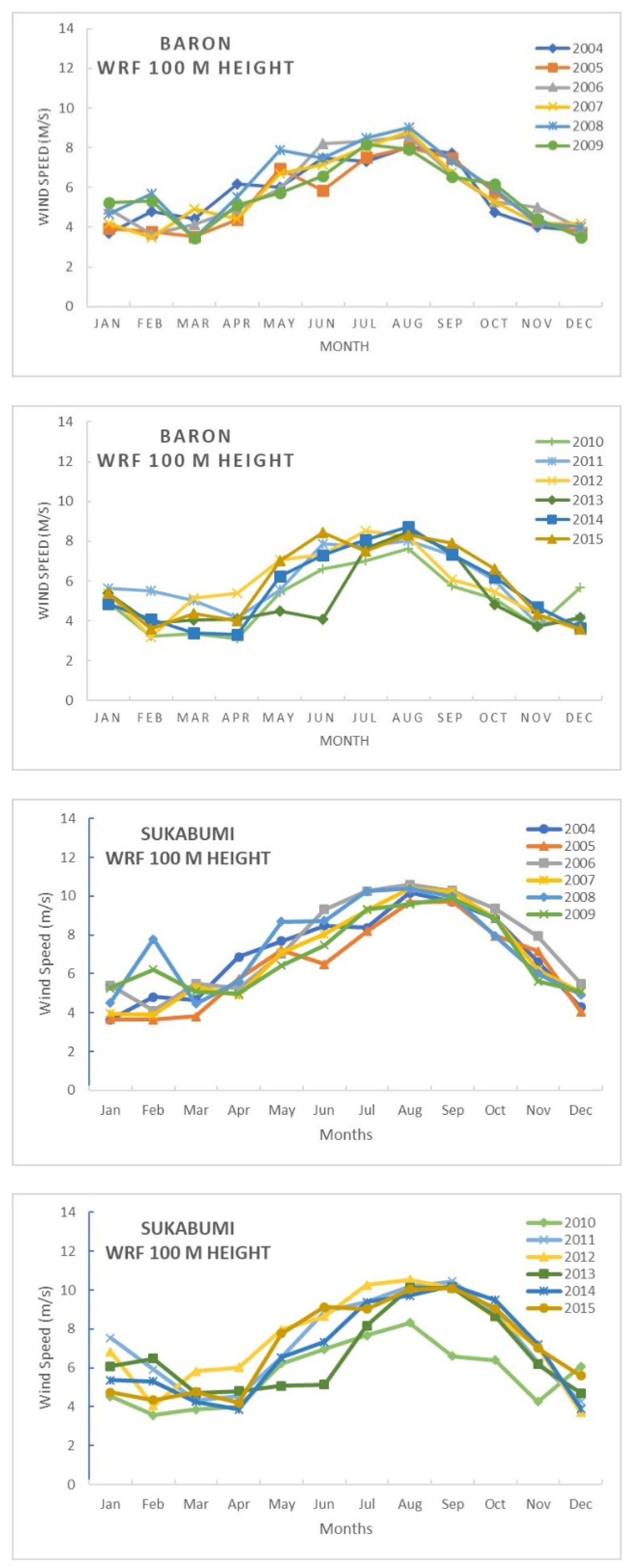
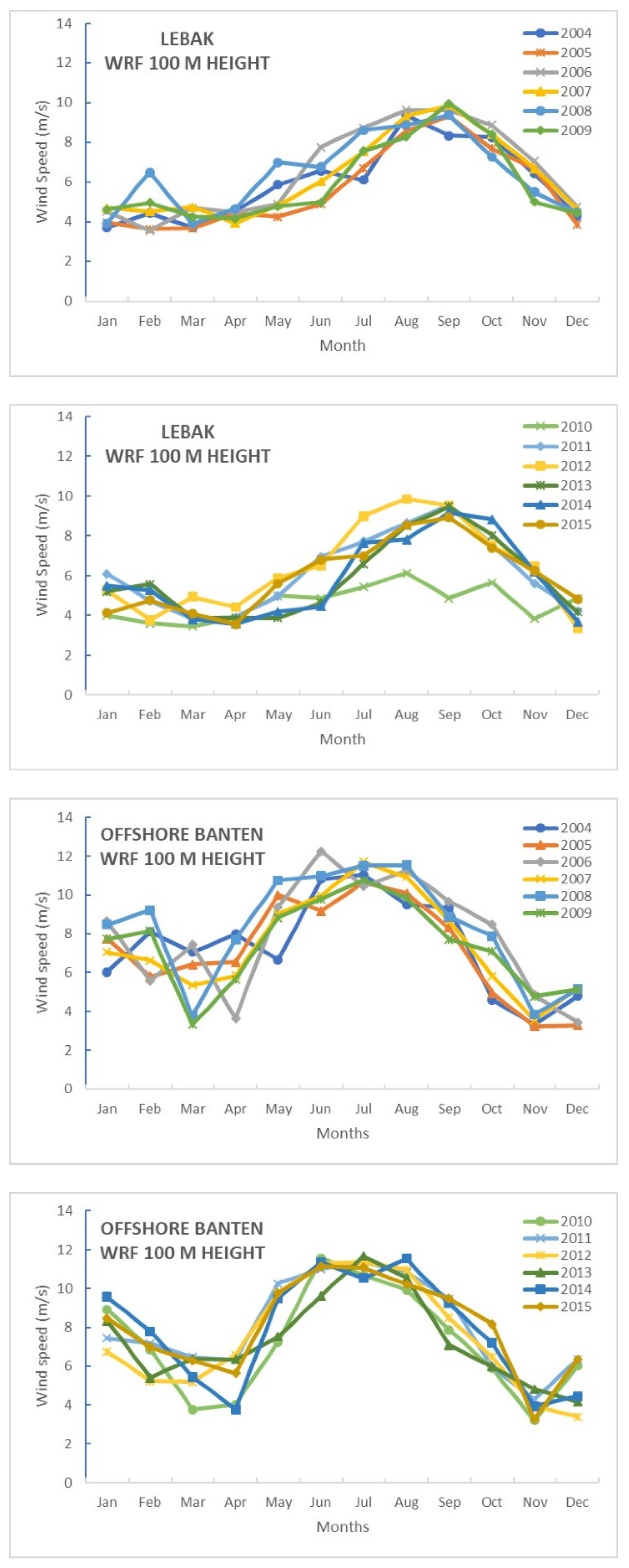
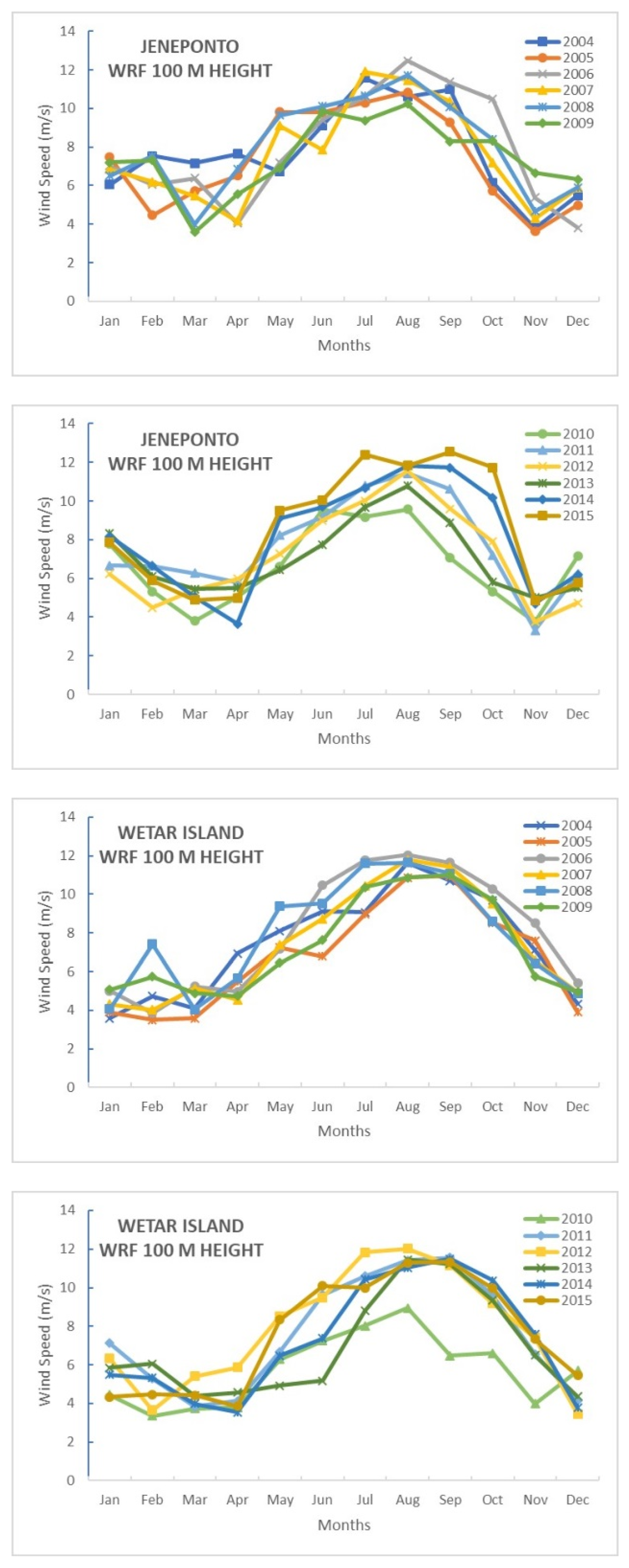
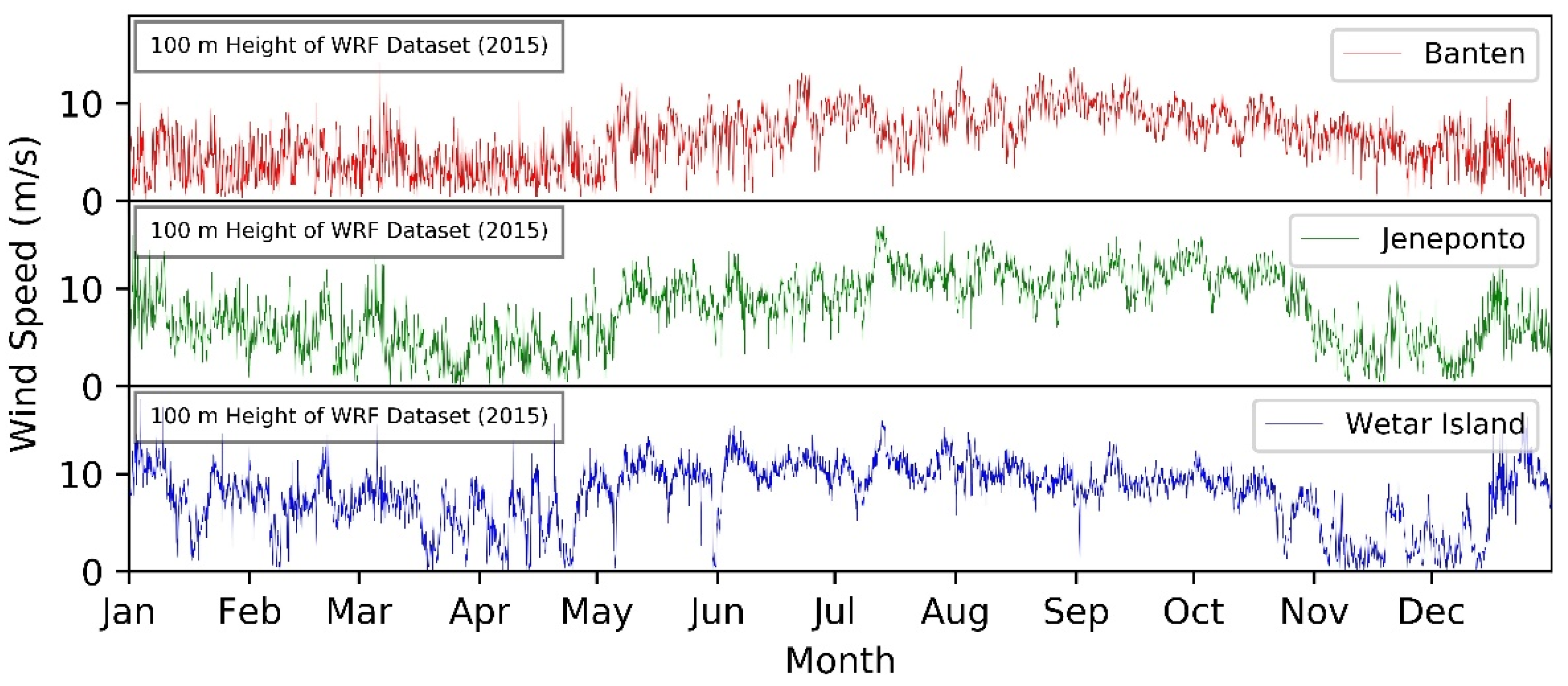
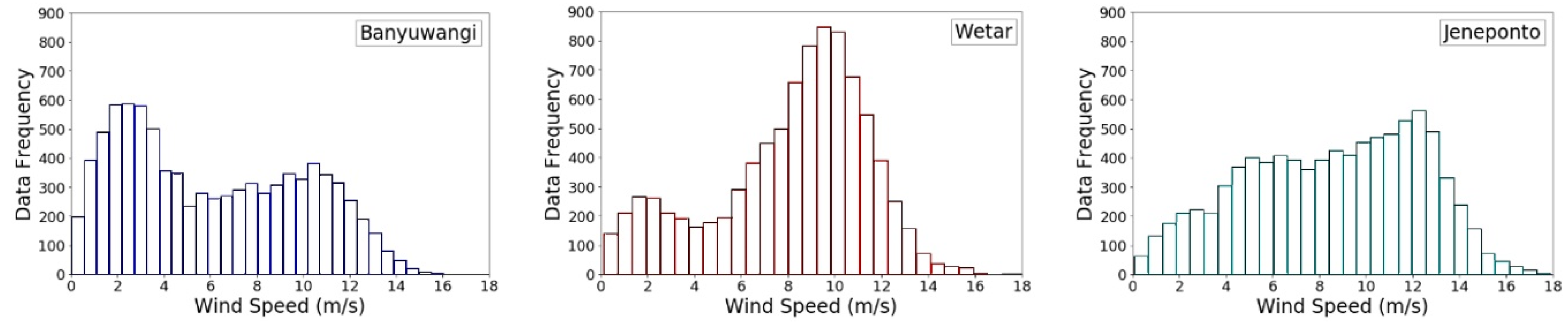
3.1. Wind Speed and Direction

Indonesia has two major seasons, rainy and dry. Monsoon wind is a dominant factor in weather changes in the country. The monthly averaged wind speed from 2004 to 2015 (Appendix A) indicated that the dry season between June and October had a higher wind speed than the rainy season between November and March. These phenomena occur in all onshore and offshore sites (Figure 2). April to May is the transition from the rainy to dry season. The weather is varied during this time.

The wind roses for the individual sites indicated that the wind direction was dominated by southeast and east–southeast winds, followed by south–southwest and east winds (Figure 3).

3.2. Comparisons of Wind Speeds Among Sites

The wind speed distribution in 2015 revealed that Banyuwangi had the highest mean onshore wind speed (6.09 m/s; Figure 4) and Jeneponto the highest offshore speed (8.51 m/s; Figure 5;

Table 2. Weibull fit distribution parameters for the studied sites (2015).

Parameter	Banyuwangi	Baron	Lebak	Sukabumi	Banten	Jeneponto	Wetar
Scale c (m/s)	6.78	6.68	6.75	5.90	7.04	9.60	9.05
Shape k	1.55	2.39	2.39	2.19	2.46	2.41	2.61
Variance	15.95	6.95	7.10	6.34	8.08	14.08	10.95
Mean wind speed (m/s)	6.09	5.92	5.98	5.23	6.56	8.51	8.04

). The offshore wind potential in both Jeneponto and Wetar Island appeared to be excellent.

The shape parameter (k) controls the width of the distribution. Higher values of k indicate a narrower frequency distribution—a steadier, less variable wind [22]. Variance refers to how much the wind speed in the wind dataset differs from the mean wind speed and thus from all other wind speed data in the dataset. Variance and the shape parameter have a strong relation, and a high shape parameter k indicates a small variance in the wind data. However, the values for k and variance in Jeneponto and Wetar Island did not seem to conform with this relation. Both the k values and variance of Jeneponto and Wetar Island were high. The reason for this phenomenon was the different wind conditions in rainy and dry seasons. A high wind speed trend is evident in dry seasons, and a low one is evident in rainy seasons. The large difference between them resulted in a high variance in these regions. The wind speed distribution in Banyuwangi, Jeneponto, and Wetar Island indicated that each has both a higher and a lower peak (Figure 6), indicating that the Weibull distribution did not fit these sites well because the distinct wind climates in rainy and dry seasons are better represented by a double-peaked distribution. Another possible reason is that the Weibull curve is an approximation of the true wind speed frequency distribution. Although the real speed distributions at many sites fit the Weibull curve well, the fit is poor in some sites.

Differences in wind distribution in the rainy and dry seasons were supplementary to the main aims of the study. The average wind speeds in the rainy and dry seasons are discussed in Section 3.1, and the wind characteristics (i.e., wind speed distributions in rainy and dry seasons) of the proposed regions were discussed in the current section. The energy production for each region was estimated as a preliminary result to select the region with the best prospects for the establishment of a wind farm. Therefore, a power production analysis was conducted.

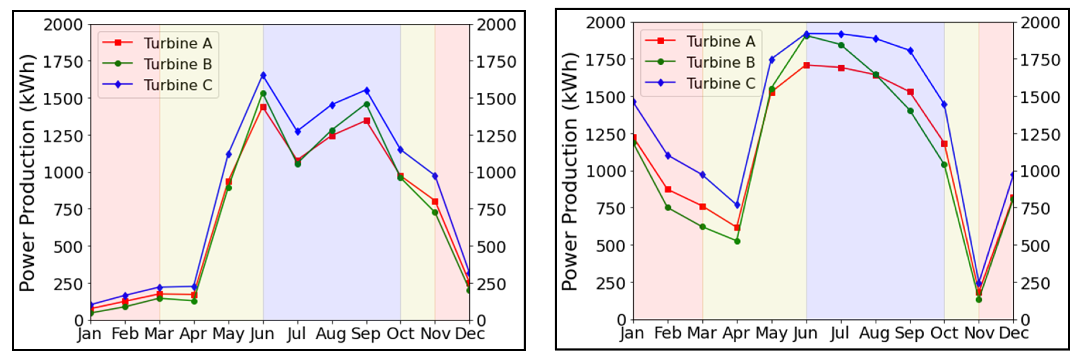
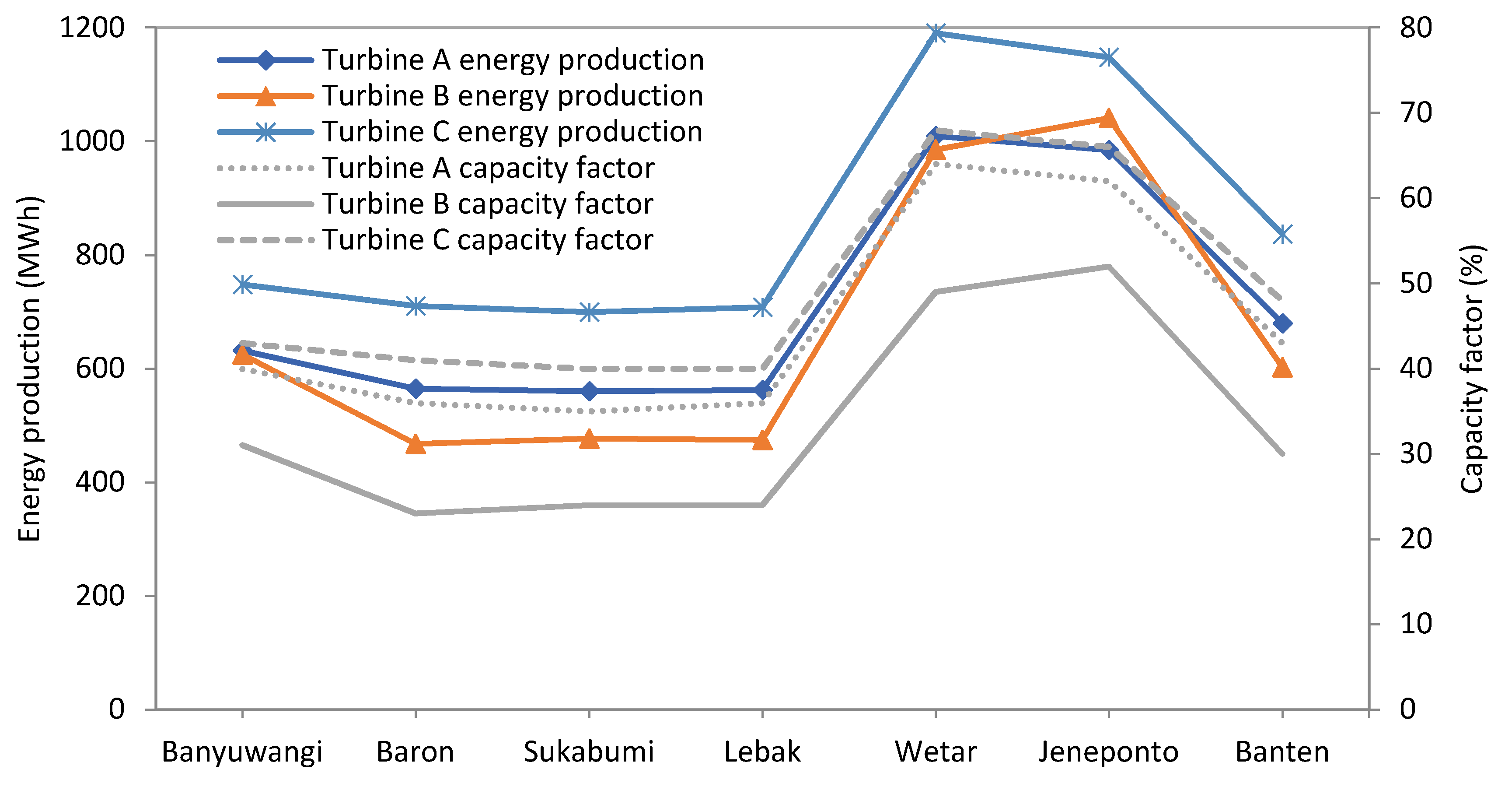
3.3. Estimated Power Production

Power production was estimated using the 2015 dataset and the power curves of the selected turbines for each site (Figure 7). Wind data at 100 m were input into the three curves. The estimated monthly average power production is depicted in Figure 8.

The results were comparable to wind speed trends; denser power production occurred in the dry season rather than in the rainy season. Wind turbine C presented the highest power production and capacity factor in all sites, followed by turbines A and B (Figure 9). This can be attributed to the fact that turbine C has the largest diameter (114 m) of the three (Table 1). Turbines with larger diameters have a larger turbine sweep area, resulting in higher power production. Another possible reason for the difference is that turbine C has the lowest cut-in and rated wind speed, enabling it to produce more power. Because the goal of the study was to determine the best scenario for building a wind farm rather than to compare the performances of wind turbines with similar specifications, the results averaged for the same rotor diameter and the impact of the wind were not discussed.

Among the sites, Wetar Island had the highest estimated power production at 1190 MWh per year and a capacity factor of 67% with turbine C, meaning that it had the greatest potential for wind energy production. Wind farm design and analysis were thus performed for Wetar Island by using WindSim.

4. Wind Farm Design and Analysis for Wetar Island

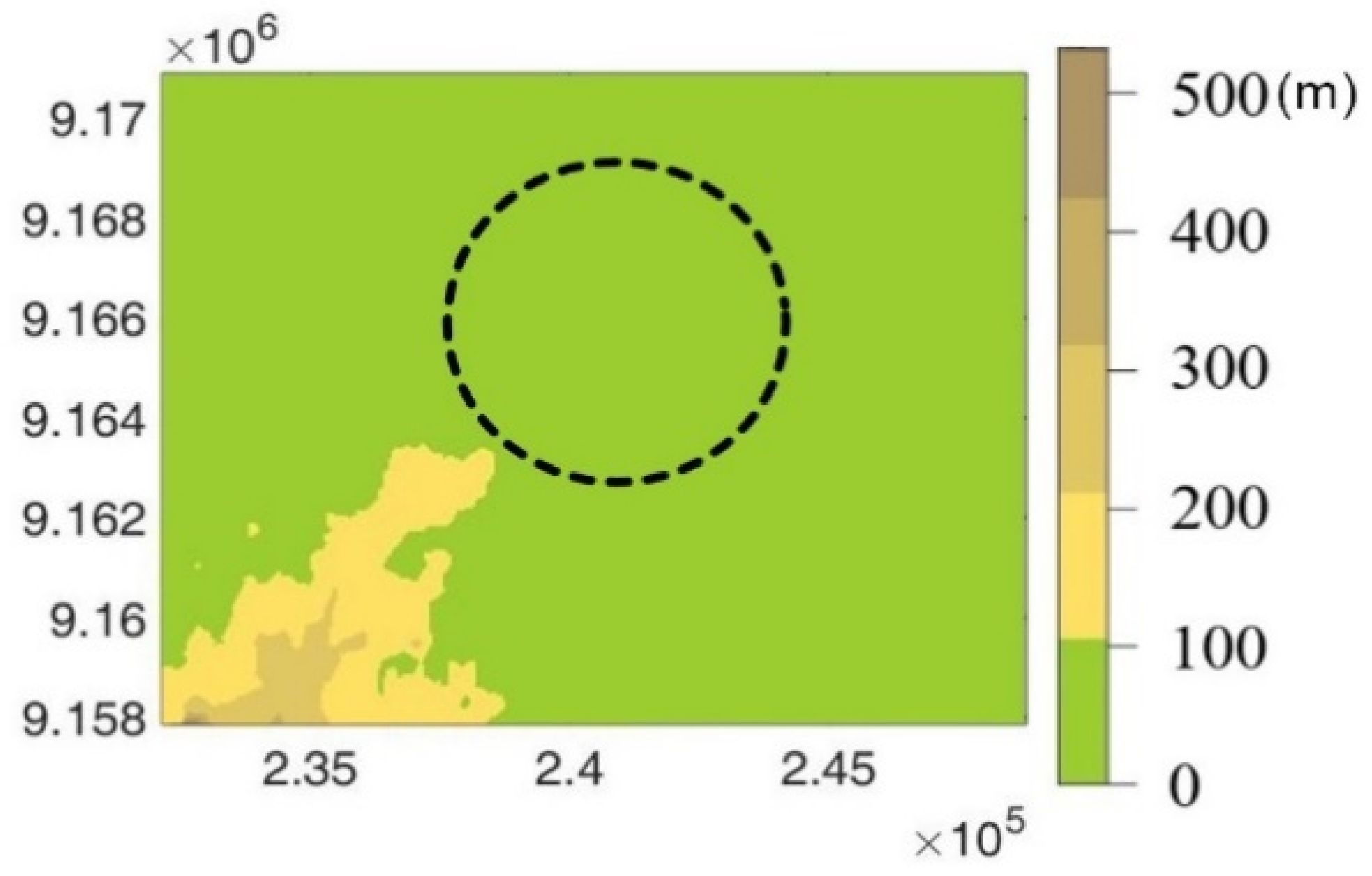
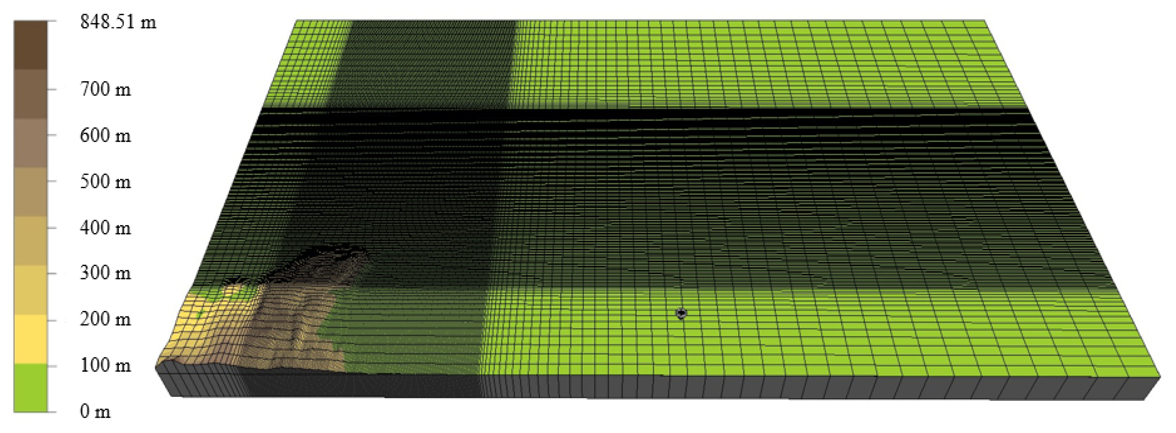
In this section, the building of terrain and wind field modules for Wetar Island by using WindSim is discussed, and the wind farm design and power production simulation are explained.

4.1. Terrain Setup

The site terrain was created in the WindSim Terrain Editor by using an orography map and a roughness map. The orography and roughness were described with counter lines on the maps, where each line provided information about the terrain. ASTER GDEM v2 Worldwide Elevation Data is a global orography map with an arc-second resolution (38.219 m). In this study, a Wetar Island orography map was derived from ASTER GDEM v2 Worldwide Elevation Data via Global Mapper software [23]. The terrain elevation of Wetar Island is depicted in Appendix B.

The roughness map was created using WindSim Terrain Editor by classifying the terrain based on roughness length (Appendix C). Globeland30 is a land cover map dataset that covers the earth from 80 N to 80 S in the baseline year of 2010. Global Mapper software was used to classify the Globeland30 map into a roughness map that was then merged with the orography map to create a terrain file. The classified landscapes and roughness lengths from Globeland30 are listed in

Table 3. Roughness length provided by Globeland30.

Landscape	Roughness Length (m)
Cultivated Land	0.050
Forest	0.180
Grassland	0.150
Shrubland	0.040
Wetland	0.003
Water Bodies	0.003
Tundra	0.200
Artificial Surfaces	0.150
Bare land	0.030
Permanent Snow and Ice	0.001
Sea	0.002

.

Sentinel-2 is optical imagery provided by the European Space Agency with a high spatial resolution (up to 10 m) for land services. The Sentinel-2 maps of Wetar Island were used to classify land use based on roughness lengths (Table 3). The orography and roughness maps were then combined into a GWS file for import into WindSim for wind farm design and analysis.

Defining the simulation domain is necessary for WindSim settings to constrain the simulation. The aim of the Terrain module is to generate a 3D model of the terrain and define mesh settings for the terrain model. The mesh of the terrain calculated in this study is presented in Figure 10 and

Table 4. Mesh of terrain.

	x	y	z	Total
Grid spacing, min–max (m)	54.1–1179.5	54.4–648.0	Variable	-
Number of cells	217	230	20	998,200

. The grid was refined, and the refinement area was centered in the northeast of Wetar Island.

4.2. Boundary Conditions

The Wind Fields module works by simulating wind fields by applying RANS equations to the 3D model mesh. The height of the boundary layer was set to 500 m, and the speed above the boundary layer was set to 10 m/s. Air density was set to 1.225 kg/m³, and the standard k-$ϵ$ model was selected as the turbulence model [24]. The general collocated velocity method was used as the solver. For a more detailed result, convergence monitoring was set in the densest cell location because the default setting was set in the center of the terrain. The number of iterations required for convergence of the spot values varied between 80 and 150, as shown in Appendix D. Usually, increasing the number of iterations was required for the residual values to reach an acceptable convergence level, which occurred after approximately 80 to 120 iterations. The variables were scaled according to the minimum and maximum values listed to the right in Appendix D. The minimum (125) and maximum (206) number of spot value iterations for a whole sector are illustrated in Appendix D.

4.3. Wind Farm Layout Optimization

The wind dataset was derived and processed from the WRF dataset at 100-m heights. The data contained the wind speed and direction, temperature, humidity, and other weather property values. The modified wind data were input into the object module as data gained from a virtual met mast located at −7.6° latitude and 126.75° longitude.

The wind resource module provides results such as mean wind speed, power density, Weibull scale and shape parameters, and wake deficit. The Jensen wake model was used because of its simplicity and relatively high accuracy [25], and the heights were set to 80, 90, and 93 m according to wind turbine specifications. Energy maps were generated using the Park Optimizer module in WindSim by combining wind speed data with the power curves of the selected turbines, as illustrated in Figure 11. Energy maps were then used as input for wind farm layout optimization.

The wind farm layout was optimized using the module Park Optimizer of WindSim. Multiple wind farm sizes were tested to assess how wind farm size influenced power production and to determine the optimal size. Wind farm sizes were classified as three variant areas: Area-1 (8.174 × 3.35 km²), Area-2 (5.5 × 3.35 km²), and Area-3 (4.1 × 3.35 km²). The size decreased from the original size in Area-1 to half that in Area-2 and one-third in Area-3. The selected wind turbine power curves and wind resource maps were input into the wind resource module, and nine variations were simulated with three wind farm sizes and three types of wind turbines.

The constraints were defined using parameters such as terrain inclination, flow inclination, shear exponent, turbulence intensity, and extreme wind. The minimal and maximal number of turbines was set to 1 and 80, respectively, with the area defined in Area-1 divided by the largest turbine diameter. The inter-turbine distance was set to 8 and 5 times the rotor diameter. The layout produced using WindSim Park Optimizer indicated that the layout typically produced a line perpendicular to the prevailing wind direction (Figure 12). An asymmetric layout order occurred because of the increase in the number of turbines. The number of turbines generated by the WindSim Park Optimizer is summarized in

Table 5. Number of turbines in a wind farm off Wetar Island calculated by WindSim Park Optimizer.

Area	Turbine A	Turbine B	Turbine C
1	61	75	48
2	42	50	35
3	32	39	27

. The turbine B required the highest number of turbines for each area. The optimized wind farm layouts are illustrated in Figure 11.

4.4. Power Production Simulations

Power estimation refers to calculating power production by combining an hourly average wind dataset with a power curve. Annual energy production (AEP) is the total hourly power production in 1 year. Power production was estimated by WindSim for all nine variations based on layout optimizations. Wind farm layouts for Area-1, -2, and -3 indicated that turbine numbers decreased with farm area (Figure 11). The results of the power production estimation indicated no significant difference in annual power production among the turbines.

The wake losses in each layout calculated by WindSim indicated that turbine B consistently had the highest wake loss, with a higher wake loss (14%) in every park layout than the other turbines (9%). Because turbine B had the smallest diameter, the Park Optimizer produced a higher number of turbines, which increased wake loss in the area.

Wind farm performance was evaluated for capacity factor and time-based availability, and power-based availability. Turbine C had the highest time-based availability and capacity factor (46% in Area-1), followed by turbine A (42% in Area-3) and turbine B (27% in Area-3). Turbine C also had the highest power-based availability (76% in Area-1), followed by turbine A (73% in Area-3) and turbine B (62% in Area-3). Turbine C appeared as the most suitable wind turbine for the wind farm on Wetar Island. The relatively low cut-in wind speed (2 m/s) and rated wind speed (10 m/s) of turbine C allow this turbine to work efficiently. Using the turbine C in Area-1 represented the best performance from the perspective of energy production.

5. Economic Analysis of Wind Farm Investment

An economic evaluation of wind farm investment is conducted in this section through an analysis of investment cost, investment indicators, and their implications for energy policy.

5.1. Wind Farm Investment Cost

The analysis of wind farm investment cost in this study was based on the assumption that the facilities were imported from Europe because Indonesia does not yet have a wind turbine manufacturer. Using the European data may provide adequate initial values to estimate the cost of each part of the wind farm. In addition, the following cost estimations (based on European data) may provide a basis for determining which scenario will be more economically viable for Wetar Island.

Investment cost comprises capital and operational expenditures. Capital expenditure involves the costs of turbines, the support system, the electrical system, and project development and management. The cost of a wind turbine with 2 to 5 MW capacity, including transportation and installation costs, can be estimated as follows [21]:

$$C_{turbine}=3.245·{10}^{3}ln\left(P\right)-412.72 \left[\mathrm{k}€\right]$$

where C_turbine is the cost of the wind turbine, and $P$ is the capacity of the wind turbine.

Support system (foundation and tower) costs include manufacturing, transportation, and installation costs. The cost of transportation and installation is assumed to be 50% of the manufacturing cost of the overall system [21,26]. The support system cost can be calculated as follows:

$$C_{support}=480·P\left(1+0.02\left(d-8\right)\right)(1+0.8·{10}^{-6}(h(\frac{D}{2}{)}^2-{10}^5)) \left[\mathrm{k}€/\mathrm{turbine}\right]$$

where C_support is the cost of the support system of the turbine, $d$ is sea depth (m), $h$ is hub height (m), and $D$ is rotor diameter (m). The cost is valid for installing wind turbines to a sea depth of 45 m and when soil properties are neglected. The electrical system functions to distribute energy generated at the wind farm to the shore area. The system is built from various components. The cost of the electrical system component ranges from 10% to 30% of the manufacturing cost depending on the electrical design and distance to the shore [21].

Collection system costs include the cost of the submarine cable used to deliver power from turbines to onshore substations at medium and high voltages. The 3-core XLPE (cross-linked polyethylene) insulated cables were selected as the collection system cable. The cost of these cables usually changes with unit length (km). The XLPE cable calculation and costs can be calculated using the turbine power rating and system voltage level as follows [21]:

$$C_{cable/km} = \alpha +\beta \times e^{\frac{\gamma ·I_n}{{10}^5}} \left[\mathrm{k}€/\mathrm{km}\right]$$

where C_cable/km is cable cost per kilometer, $\alpha$ = 52.08, $\beta$ = 75.51, $\gamma$ = 234.34 are coefficients of different cable voltage levels, and $I_n$ is cable capacity. The radial, star, and circle are common electrical layouts for wind farms. In this case, the radial electrical layout was chosen due to the number of turbines, which varied from 4 to 12 for each line depending on the layout. A maximum of 12 turbines was determined by the maximum cable capacity of the XLPE cable type [21]. Total cable cost can be calculated as follows:

$$C_{cable} = C_{cable/km} m{l}_{cable} \left[\mathrm{k}€\right]$$

where $l_{cable}$ is cable length in kilometers. A 40-m cable is recommended as a supplementary cable extension [27]. Offshore cables must be buried for safety reasons and to prevent external damage. The cost of burying cable changes with unit length (km). Following Quinonez-Varela et al. [28], the cost of burying cable is as follows:

$$C_{burying} = 273 3 l_{cable} \left[\mathrm{k}€\right]$$

Onshore substation components mainly consist of transformers, high voltage busbars, switch gears, and backup generators. The cost of a substation is a function of wind farm capacity. The cost of a substation is 50 k€/MW [27]. Power factor correction devices, such as shunt reactors, static VAR compensators, and STATCOMs, are necessary to increase power efficiency during electricity distribution. The cost model was calculated as follows [27]:

$$\{\begin{array}{c}{C}_{shunt-reactor}=2.556 \mathrm{k}€/\mathrm{MVAr}\\ C_{SVC}=6.39 \mathrm{k}€ + 63.9 \mathrm{k}€/\mathrm{MVAr}\\ C_{STATCOM}=128 \mathrm{k}€/\mathrm{MVAr}\end{array}$$

Total substation cost can therefore be calculated as follows:

$$C_{substation} = 50 \left[\mathrm{k}€\right]/\mathrm{MW} + C_{shunt-reactor} + C_{SVC} + C_{STATCOM}$$

The transmission line is the cable connecting the collection line to a substation. Because the cable must transfer electricity from the turbine, this price is different from that for the collection cable system. The transmission line cost is $673.6 \mathrm{k}€/\mathrm{km}$ for $630-{\mathrm{mm}}^2$ and $150-\mathrm{kV}$ based on Indonesia’s transmission line standards. Grid connection cost is considered a function of installed wind power [27] and was calculated as follows [21]:

$$C_{GC} = 8.047 .0P^{1.66}$$

where $C_{GC}$ is grid connection cost and P is installed capacity.

Project development, management, and other costs vary depending on project details. The estimation of this cost usually includes insurance, employee salaries, and engineering design of approximately 280.38 USD/MW [21]. The operational expenditure of a wind farm covers operational and maintenance costs, including administrative costs, insurance premiums, and royalties. This cost is usually estimated at 1.9% of the CapEx per year over a 20-year farm life-span [21].

The capital and operational expenditures for each scenario were calculated to determine which scenario is the most economically viable. The cost breakdown of the wind farm indicated that the highest total CapEx for Area-1 was for the turbine B layout at approximately 539 million USD, whereas that for Area-2 and Area-3 was for the turbine B at 390 million USD and 286 million USD, respectively (

Table 6. Cost breakdown of wind farms off Wetar Island by area and turbine (all costs in thousands of USD).

Area		1			2			3
Type of Turbine	A	B	C	A	B	C	A	B	C
CapEx
Wind turbine	121,716.6	229,293.3	117,685.6	83,804.9	152,862.2	85,812.5	63,851.4	119,232.5	66,198.2
Support system a	103,710.4	155,467.7	95,764.0	71,407.2	103,645.1	69,827.9	54,405.5	80,843.2	53,867.2
Electrical system
Collection system
Inner cable	22,528.1	25,193.7	19,666.6	14,215.0	18,074.3	13,179.2	10,623.2	8870.6	9663.9
Buried cable	21,883.0	24,450.6	19,769.2	15,861.2	20,703.9	15,004.5	12,907.3	11,106.7	12,275.8
Onshore substation	11,199.3	15,427.0	10,205.3	7729.9	10,320.6	7441.9	5902.8	8054.6	5741.9
Transmission line	36,656.6	40,756.1	36,845.5	38,056.2	52,028.7	37,471.0	36,146.2	32,647.4	36,759.8
Grid connection	28.5	42.8	33.9	28.5	42.8	33.9	28.5	42.8	33.9
Project development	30,785.7	48,365.6	26,916.5	21,196.7	32,243.7	19,626.6	16,149.9	25,150.1	15,140.5
Total	348,508.2	538,996.7	326,886.7	252,299.6	389,921.4	248,397.4	200,014.7	285,947.9	199,681.3
OpEx (per year)	6.6	10.2	6.2	4.8	7.4	4.7	3.8	5.4	3.8

^a Average sea depth was set at 25 m for Wetar Island.

). Turbine and support system costs comprised most of the total CapEx costs, with values ranging from 32% to 42% for turbine cost and 28% to 29% for support system cost. The cost for the electrical system was divided into collection system cost, onshore substation cost, transmission line, and grid connection. The main cost for the electrical system was the cable cost. This cost can be divided into the cable used for each turbine (collection system cable) and the transmission line. The cable length was estimated by calculating the distance for each turbine and then adding 40 m for supplementary use. The radial layout was chosen because it is more economical than the ring or star layout [28]. The wind farm cabling layout is presented in Figure 13. The highest cost in the electrical system was the transmission line, which depended on cable length and the diameter between cables.

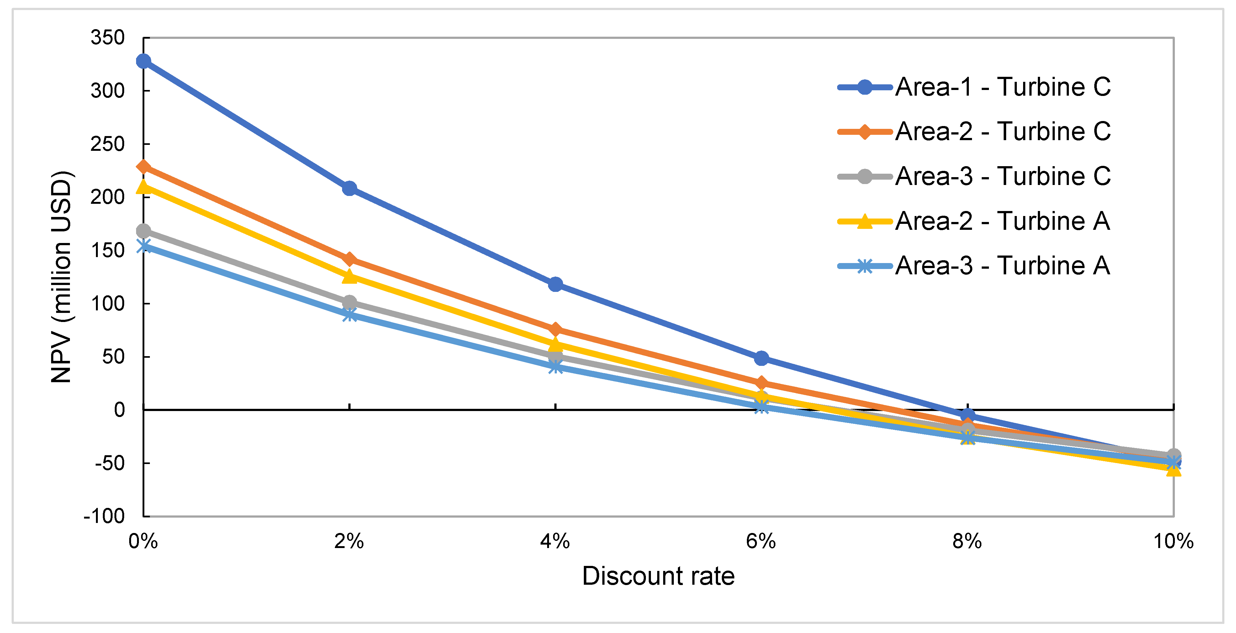
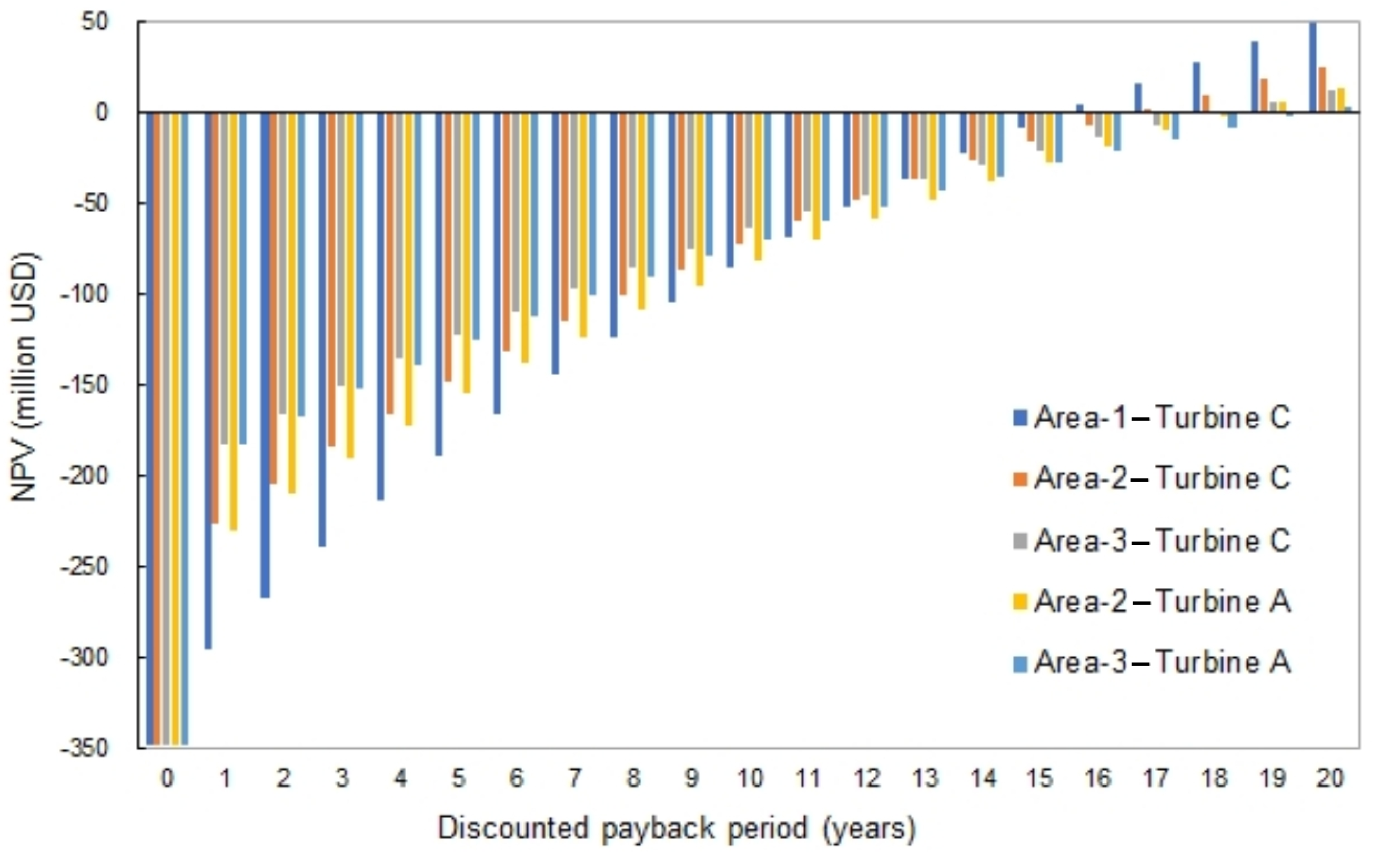
5.2. Investment Indicator

The NPV (net present value), LCOE (Levelized Cost of Electricity), and DPBP (Discounted Payback Period) were used in this study to evaluate the wind farm investment. NPV represents the difference between the present value of cash inflows and the present value of cash outflows over a period of time. Positive NPV values represent economic viability [21]. NPV can be expressed by:

$$\mathrm{NPV} = -C_{CAPEX} + {\displaystyle \sum _{t=1}^T}\frac{\mathit{netCashFlow}\left(t\right)}{{(1+r)}^t}$$

where $C_{CAPEX}$ is the total capital expenditure, $T$ is the lifespan of the wind farm, and $r$ is the annual discount rate.

LCOE represents the offshore wind farm net present value divided by the wind farm lifetime. LCOE can be calculated as follows:

$$\mathrm{LCOE}=\frac{{\displaystyle {\sum }_{t=1}^T\frac{C_{CapEx}(t)+C_{OpEx}(t)}{{(1+r)}^t}}}{{\displaystyle {\sum }_{t=1}^T\frac{net\mathrm{AEP}}{{(1+r)}^t}}}$$

where $C_{OpEx}\left(t\right)$ is the operational expenditure of wind farms for the year of $t$, the netAEP is the total estimated energy production for one year.

DPBP represents the time required for the cumulative profit to equal the cumulative cost, considering the discount rate. DPBP is applied when the discount rate is greater than zero. DPBP can be calculated as follows:

$$\mathrm{DPBP}=\frac{ln\left(\frac{1}{1-\frac{C_{CapEx}\times r}{NetCashFlow}}\right)}{ln\left(1+r\right)}$$

According to Indonesian regulations, the feed-in-tariff (FIT) for wind energy cannot be higher than the regional cost of provision [29]. The regional cost of provision near Sidrap Wind Farm was approximately 0.08 USD/kWh. The projected lifespan of the proposed wind farm was set at 20 years. Discount rates of 2%, 6%, and 10% were considered in the sensitivity analysis.

The AEP of farms was calculated using the WindSim results. The annual revenue was the product of the multiplication of AEP and FIT. The annual revenue increased with AEP; Area-1 with wind turbine B produced the highest annual revenue.

NPV analysis indicated that wind turbine C always had a positive (i.e., feasible) NPV value, whereas turbine B always had a negative (infeasible) value. The highest NPV was for the wind turbine C in Area-1 at USD 48.7 million. Variations in the discount rate revealed the sensitivity of NPV change (Figure 14). Area-1 had a higher NPV compared with others with a discount rate lower than 6%. A 6% discount rate appeared to be the highest acceptable rate. A discount rate higher than 6% led to negative NPV, making the project infeasible.

LCOE for various wind farm sizes off Wetar Island indicated that LCOE slightly increased as farm size dwindled. The lowest LCOE was 0.082 USD/kWh for the turbine C in Area-1, followed by 0.085 USD/kWh in Area-2. Turbine A had slightly higher LCOE than turbine C did, whereas turbine B had substantially higher LCOE. The lowest LCOE at 0.082 USD/kWh was still higher than the FIT for wind power in Indonesia at 0.08 USD/kWh. A higher FIT would be required for Indonesia to draw investment in wind energy.

DPBP can be observed at the point where NPV starts to have a positive value, which means the farm is profitable. DPBPs for five feasible scenarios indicated that turbine C had the shortest DPBP at 16 and 17 years in Area-1 and Area-2, respectively (Figure 15).

5.3. Implications for Energy Policy

The LCOE of wind farms off Wetar Island was estimated as 0.082 USD/kWh, which is higher than the current FIT for wind power in Indonesia. When considering the external costs of fossil fuels, such as costs from global warming and health detriment, wind farms off Wetar Island may be a cost-effective and more sustainable option for power generation in comparison with power generation from fossil fuels with LCOE between 0.07 and 0.15 USD/kWh in Indonesia [30]. In addition, the 0.08 USD/kWh FIT for wind power in Indonesia is relatively low (Figure 16). Increasing the FIT may be required to promote offshore wind energy production in Indonesia. Total energy subsidies in Indonesia were estimated at 27.7 billion USD in 2014 (about 3% of GDP), almost 6% of the 493 billion USD in global subsidies to fossil fuels that same year [31]. Moving subsidies from fossil fuels toward renewables would be required to facilitate the use of low-carbon wind energy without increasing the financial burden on the country.

6. Conclusions

In this study, wind power potential in Indonesia was evaluated at four onshore and three offshore sites. The novel findings are as follows:

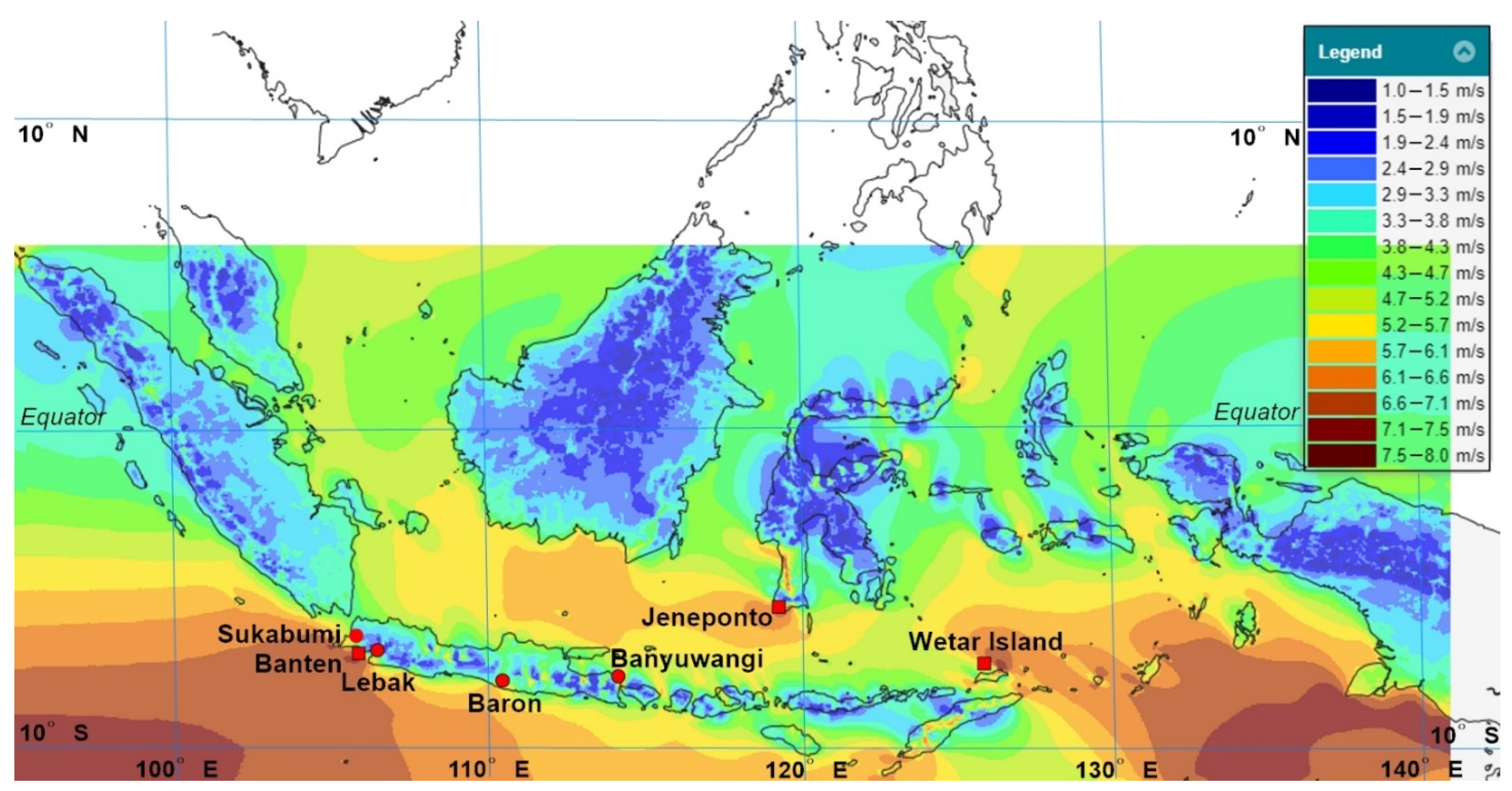
• The tropical regions of Southeast Asia are generally characterized by scarce wind resources. However, the mean annual wind speeds offshore Jeneponto and Wetar Island reached 8.51 m/s and 8.04 m/s, respectively, in 2015. The capacity factor and power-based availability of a wind farm for each location reached 46% and 76%, respectively, exhibiting an excellent potential for wind energy production;
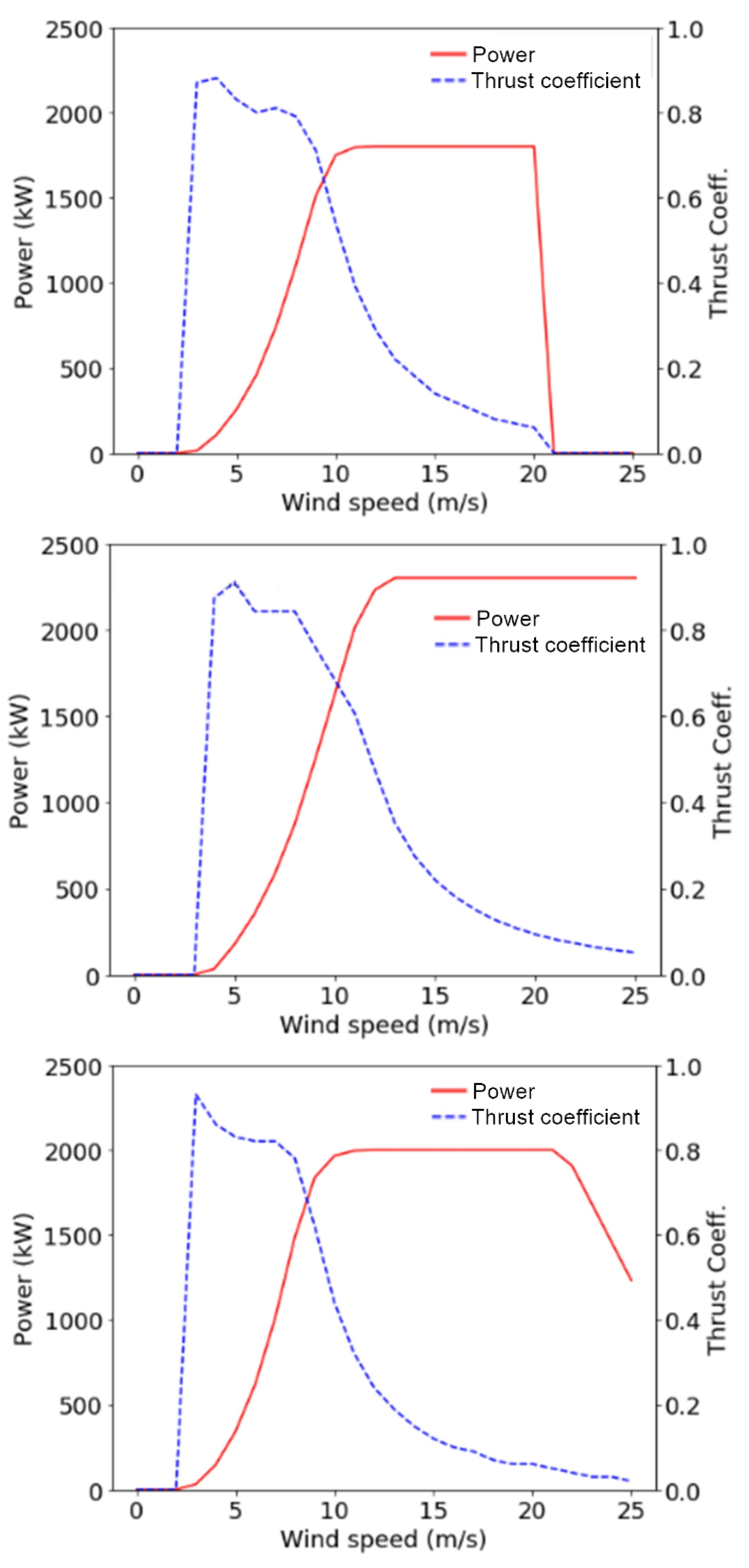
• Using wind turbine C with the highest hub height, largest rotor diameter, and lowest cut-in and rated wind speed achieved the largest capacity factor among the selected commercial wind turbines, indicating that these features may enhance the efficiency of wind power generation;
• Wake loss was affected more by the performance of individual turbines rather than the size of the farm. Using turbines with smaller rotor diameters often leads to a layout with a higher number of turbines, increasing wake loss in the area;
• The LCOE of various wind farm sizes indicated that LCOE slowly increased as farm size shrank. Increasing the size of a wind farm may enhance the economic effectiveness of investment;
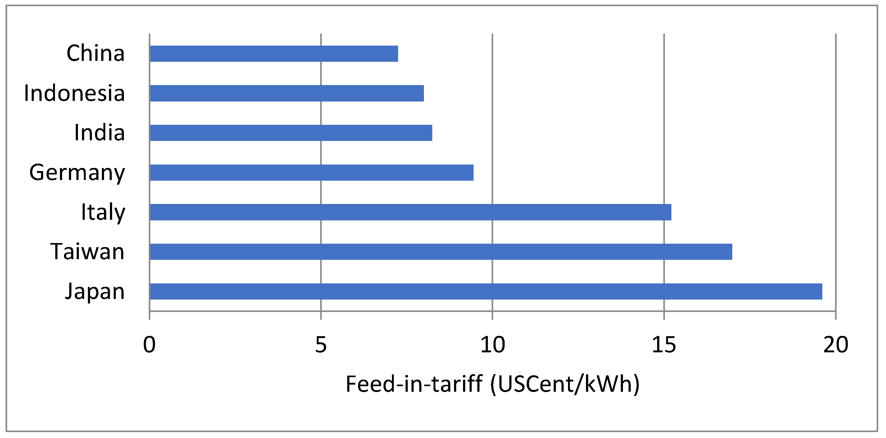
• The LCOE of offshore wind farms can be as low as 0.082 USD/kWh, which is comparable to that of power generation from fossil fuels (between 0.07 and 0.15 USD/kWh) in Indonesia. The current FIT for wind power (0.08 USD/kWh) would require enhancement to attract investment.

The cost of wind energy has considerably reduced to a level now comparable to that of fossil fuels. This study demonstrated that offshore wind energy has become a cost-effective low-carbon option for power generation. Moving subsidies from fossil fuels toward renewables would facilitate the use of low-carbon wind energy without increasing the financial burden on the country.

This study provides vital findings for wind farm stakeholders. First, increasing the size of a wind farm may enhance its economic effectiveness. Second, using turbines with larger rotor diameters may help minimize turbine number and wake loss. In contrast to past findings indicating that the tropical regions of Southeast Asia have sparse wind energy resources, this study reveals that this region has considerable wind energy potential. This finding may inform regional and international low-carbon policy in addition to promoting further research activities and investment in wind power generation in this region.

References

1. UNEP. Emissions Gap Report 2019; United Nations Environment Programme (UNEP): Nairobi, Kenya, 2019. [Google Scholar]
2. Lin, Y.R. Global Coal-Fired Power Generation is Increasing While European and American Investors Raise the Stakes, Awakening News Networks. Available online: https://udn.com/news/story/6811/4298905?from=udn-catelistnews_ch2 (accessed on 20 January 2020).
3. IRENA; ACE. Renewable Energy Outlook for ASEAN: A REmap Analysis; International Renewable Energy Agency (IRENA): Abu Dhabi, United Arab Emirates; ASEAN Centre for Energy (ACE): Jakarta, Indonesia, 2016. [Google Scholar]
4. Yuliani, D. Is feed-in-tariff policy effective for increasing deployment of renewable energy in Indonesia? In The Political Economy of Clean Energy Transitions; Arent, D., Arndt, C., Miller, M., Tarp, F., Zinaman, O., Eds.; Oxford University Press: Oxford, UK, 2017; Available online: https://www.oxfordscholarship.com/view/10.1093/oso/9780198802242.001.0001/oso-9780198802242-chapter-8?print=pdf (accessed on 2 April 2019).
5. Lutgens, F.K.; Tarbuck, E.J. The Atmosphere: An Introduction to Meteorology; Prentice Hall: New York, NY, USA, 2001. [Google Scholar]
6. Hardianto, T.; Supeno, B.; Saleh, A.; Setiawan, D.K.; Gunawan; Indra, S. Potential of Wind Energy and Design Configuration of Wind Farm on Puger Beach at Jember Indonesia. Energy Procedia 2017, 143, 579–584. [Google Scholar] [CrossRef]
7. Martosaputro, S.; Murti, N. Blowing the Wind Energy in Indonesia. Energy Procedia 2014, 47, 273–282. [Google Scholar] [CrossRef] [Green Version]
8. Carvalho, D.; Rocha, A.; Gómez-Gesteira, M.; Silva-Santos, C. Off-shore winds and wind energy production estimates derived from ASCAT, OSCAT, numerical weather prediction models and buoys e a comparative study for the Iberian Peninsula Atlantic coast. Renew. Energy 2017, 102, 433–444. [Google Scholar] [CrossRef]
9. Mattar, C.; Borvarán, D. Off-shore wind power simulation by using WRF in the central coast of Chile. Renew. Energy 2016, 94, 22–31. [Google Scholar] [CrossRef]
10. De Linaje, N.G.-A.; Mattar, C.; Borvarán, D. Quantifying the wind energy potential differences using different WRF initial conditions on Mediterranean coast of Chile. Energy 2019, 188, 116027. [Google Scholar] [CrossRef]
11. Grell, G.; Peckham, S.; Schmitz, R.; McKeen, S.; Frost, G.; Skamarock, W.; Eder, B. Fully coupled “online” chemistry within the WRF model. Atmos. Environ. 2005, 39, 6957–6975. [Google Scholar] [CrossRef]
12. Skamarock, W.; Klemp, J.; Dudhia, J.; Gill, D.; Barker, D.; Duda, M.; Huang, X.; Wanf, W.; Powers, J. A Description of the Advanced Research WRF Version 3 [Online]. 2008. Available online: http://www2.mmm.ucar.edu/wrf/users/docs/arw_v3.pdf (accessed on 13 April 2021).
13. Ulazia, A.; Saenz, J.; Ibarra-Berastegui, G. Sensitivity to the use of 3DVAR data assimilation in a mesoscale model for estimating off-shore wind energy potential. A case study of the Iberian northern coastline. Appl. Energy 2016, 180, 617–627. [Google Scholar] [CrossRef]
14. Olaofe, Z. Quantification of the near-surface wind conditions of the African coast: A comparative approach (satellite, NCEP CFSR and WRF-based). Energy 2019, 189, 116232. [Google Scholar] [CrossRef]
15. Salvação, N.; Soares, C.G. Wind resource assessment offshore the Atlantic Iberian coast with the WRF model. Energy 2018, 145, 276–287. [Google Scholar] [CrossRef]
16. Prósper, M.A.; Otero-Casal, C.; Fernández, F.C.; Miguez-Macho, G. Wind power forecasting for a real onshore wind farm on complex terrain using WRF high resolution simulations. Renew. Energy 2019, 135, 674–686. [Google Scholar] [CrossRef]
17. Bansal, J.C.; Farswan, P. Wind farm layout using biogeography based optimization. Renew. Energy 2017, 107, 386–402. [Google Scholar] [CrossRef]
18. Patel, J.; Savsani, V.; Patel, V.; Patel, R. Layout optimization of a wind farm using geometric pattern-based approach. Energy Procedia 2019, 158, 940–946. [Google Scholar] [CrossRef]
19. Park, J.; Law, K.H. Layout optimization for maximizing wind farm power production using sequential convex programming. Appl. Energy 2015, 151, 320–334. [Google Scholar] [CrossRef]
20. EMD. WindPROSPECTING: Wind Energy Resources of Indonesia. EMD International A/S. Available online: http://indonesia.windprospecting.com/ (accessed on 24 March 2016).
21. Cali, U.; Erdogan, N.; Kucuksari, S.; Argin, M. Techno-economic analysis of high potential offshore wind farm locations in Turkey. Energy Strategy Rev. 2018, 22, 325–336. [Google Scholar] [CrossRef]
22. Brower, M. Wind Resource Assessment: A Practical Guide to Developing a Wind Project; John Wiley & Sons: New York, NY, USA, 2012. [Google Scholar]
23. NASA/METI/AIST/Japan Space Systems; U.S./Japan ASTER Science Team. ASTER Global Digital Elevation Model [Data Set]. NASA EOSDIS Land Processes DAAC. 2009. Available online: https://doi.org/10.5067/ASTER/ASTGTM.002 (accessed on 6 December 2020).
24. Yakhot, V.; Orszag, S.A.; Thangam, S.; Gatski, T.B.; Speziale, C.G. Development of turbulence models for shear flows by a double expansion technique. Phys. Fluids A Fluid Dyn. 1992, 4, 1510–1520. [Google Scholar] [CrossRef] [Green Version]
25. Shakoor, R.; Hassan, M.Y.; Raheem, A.; Wu, Y.-K. Wake effect modeling: A review of wind farm layout optimization using Jensen’s model. Renew. Sustain. Energy Rev. 2016, 58, 1048–1059. [Google Scholar] [CrossRef]
26. Dicorato, M.; Forte, G.; Pisani, M.; Trovato, M. Guidelines for assessment of investment cost for offshore wind generation. Renew. Energy 2011, 36, 2043–2051. [Google Scholar] [CrossRef]
27. Gonzalez-Rodriguez, A.G. Review of offshore wind farm cost components. Energy Sustain. Dev. 2017, 37, 10–19. [Google Scholar] [CrossRef]
28. Quinonez-Varela, G.; Ault, G.W.; Anaya-Lara, O.; McDonald, J.R. Electrical collector system options for large offshore wind farms. IET Renew. Power Gener. 2007, 1, 107–114. [Google Scholar] [CrossRef]
29. MMRI. Ministry of Mineral Resources of Indonesia Regulation No. 50/2017; Ministry of Mineral Resources of Indonesia (MMRI): Jakarta, Indonesia, 2017.
30. IRENA. Renewable Energy Prospects: Indonesia. International Renewable Energy Agency (IRENA). Available online: https://irena.org/2017 (accessed on 24 April 2020).
31. IEA. Fossil Fuel Subsidy Database. Available online: http://www.worldenergyoutlook.org/resources/energysubsidies/fossilfuelsubsidydatabase/ (accessed on 24 February 2016).
32. MEAROC. Feed-In Tariff of Electricity Generated from Renewable Energy Sources and its Calculation Formula; Ministry of Economic Affairs of the Republic of China (MEAROC): Taipei, Taiwan, 2019.
33. OECD. Renewable Energy Feed-In Tariffs. Available online: https://stats.oecd.org/Index.aspx?DataSetCode=RE_FIT (accessed on 24 April 2020).
Figure 1. WRF map of Indonesia generated using the ERA-Interim data map (2004–2015) [20]. The locations of onshore sites in Banyuwangi, Baron, Lebak, and Sukabumi (circular points) and offshore sites in Jeneponto, Wetar Island, and Banten (square points) are indicated. The colored contours denote horizontal wind speeds at a height of 100 m.
Energies 14 02652 g001
Figure 2. Average wind speed (2004–2015) for dry and rainy seasons in onshore (left) and offshore (right) sites.
Energies 14 02652 g002
Figure 3. Wind roses in 2015 for the onshore Banyuwangi, Baron, Lebak, and Sukabumi sites (top, left to right) and offshore Wetar, Jeneponto, and Banten sites (bottom, left to right).
Energies 14 02652 g003
Figure 4. WRF wind speed at 100 m for onshore sites in 2015.
Energies 14 02652 g004
Figure 5. WRF wind speed at 100 m for offshore sites in 2015.
Energies 14 02652 g005
Figure 6. Wind speed distribution for Banyuwangi, Wetar, and Jeneponto.
Energies 14 02652 g006
Figure 7. Power curves of selected wind turbines A (top), B (middle), and C (bottom).
Energies 14 02652 g007
Figure 8. Monthly average power production estimated using the power curve of three selected wind turbines in Banyuwangi (left) and Wetar Island (right) (2015 data). The red-colored region indicates the rainy season, blue indicates the dry season, and yellow indicates the transition seasons between the dry and rainy season and vice versa.
Energies 14 02652 g008
Figure 9. Power production and capacity factor of the turbines at all sites.
Energies 14 02652 g009
Figure 10. Terrain model grid of Wetar Island with the wind data source location.
Energies 14 02652 g010
Figure 11. Energy maps and optimized wind farm layouts off Wetar Island using turbine A (top), turbine B (middle), and turbine C (bottom) in Area-1, Area-2, and Area-3, respectively.
Energies 14 02652 g011
Figure 12. Symmetric (left) and asymmetric (right) wind farm layout off Wetar Island.
Energies 14 02652 g012
Figure 13. Wind farm cabling for wind turbine A in Area-1. The blue lines represent collection system cables, and the black lines represent transmission lines. The square represents the onshore substation.
Energies 14 02652 g013
Figure 14. Sensitivity of NPV for different discount rates at the proposed wind farms off Wetar Island.
Energies 14 02652 g014
Figure 15. Discounted payback period for five feasible scenarios for wind farms off Wetar Island.
Energies 14 02652 g015
Figure 16. Comparison of feed-in tariffs for electricity from wind energy in selected countries in 2017 [29,32,33].
Energies 14 02652 g016