Reinforcement Learning Path Planning Method with Error Estimation

Abstract

Path planning is often considered as an important task in autonomous driving applications. Current planning method only concerns the knowledge of robot kinematics, however, in GPS denied environments, the robot odometry sensor often causes accumulated error. To address this problem, an improved path planning algorithm is proposed based on reinforcement learning method, which also calculates the characteristics of the cumulated error during the planning procedure. The cumulative error path is calculated by the map with convex target processing, while modifying the algorithm reward and punishment parameters based on the error estimation strategy. To verify the proposed approach, simulation experiments exhibited that the algorithm effectively avoid the error drift in path planning.

1. Introduction

Path planning is often utilized to design the optimal trajectory from the start point to the destination. To achieve this goal, various information is required such as the geometric and dynamic information [1], environment map [2], initial state and target state [3]. Furthermore, due to different requirements [4], the collision-free paths are also calculated through multidimensional based on structured scenarios [5].

So far, path planning methods consist of heuristic searching, sampling planning, and model-dependent methods [6]. However, none of the aforementioned methods considers the localization uncertainty issue. In scenarios of GPS denied environments, noisy odometer measurements often lead to unbounded positioning errors. Hence, optimization based on error statistical characteristics is considered, by using the machine learning method. Ref. [7] assumed the background knowledge of the distances is known, and the planning process only needs to update the entries of Q-Table once with four derived attributes. Ref. [8] formulated the behavioral rules of the agent according to the prior environment characteristics. Based on Dubin’s vehicle model, ref. [9] used the dynamic MPNet to generate a suboptimal path. Ref. [10] proposed the integral reinforcement learning path planning solution in continuous state space. Ref. [11] combined soft mobile robot modeling with iterative learning control, and considered adaptive motion planning and trajectory tracking algorithms as its kinematic and dynamic states. Ref. [12] proposed a path planning method called CNPP-Convolutional Network. The method allows multipath planning at one time, that is, a multipath search can be realized through a single prediction iteration of the network. Although the machine learning-based methods were well studied, the method which considers the positioning error is still missing.

Furthermore, traditional planning methods rarely perform fault-tolerant on the control strategy [13]. Therefore, it is quite challenging to plan the path without considering the inevitable errors. Ref. [14] demonstrated a fully convolutional network method to learn human perception, with a real-time RRT* planner to enhance the planner’s ability. By the deep Q-networks calculated from the dense network framework, ref. [15] solved the robot drift issue. Ref. [16] improved the hybrid reciprocating speed obstacle method with dynamic constraints. However, the current approach does not consider the mechanism of initial cumulative error to reduce the positioning uncertainty, which is unacceptable for robots with fine operations.

The proposed approach bridges gaps between the localization process with theoretical qualitative analysis, and the path planning process with the reinforcement learning algorithm, to address cumulative error issues during the navigation procedure. In this paper, an improved path model based on error strategy is established, and the optimal path is calculated through offline learning. The core idea of this paper is that the robot tracking forward will produce the cumulative error drift relative to set path, and the change of set path will also change the drift error. Based on this, the error drift is considered and processed in process of path planning, which can effectively reduce the tracking error.

This paper is organized as follows: Section 2 introduces the statistical characteristics of localization error. Section 3 presents the reinforcement learning-based path planning framework. Section 4 analyzes the effect of the planning algorithm and Section 5 concludes the paper and discusses possible directions for future work.

2. Background

Normally, the robot uses GPS combined with attitude and inertial sensors (gyroscopes and accelerometers) for localization. In the absence of GPS scenarios, the position is calculated by the dead-reckoning approach. It is assumed that the errors in IMU come from measuring white noise only, ignoring Shura period oscillations, Foucault period oscillations, and Earth period oscillations. Assuming the noise is distributed with independent and identical distribution (IID) in polar coordinates, the robot needs to regularly correct errors to achieve high-precision navigation.

Hence, the main challenge is the drift caused by noisy measurement, whereas the localization error accumulates nonlinearly through distance. Based on our original work [17], a statistical formula concerning the noisy measurement is proposed, to obtain the cumulative error growth rate. The solution is as follows:

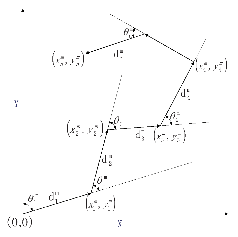
In polar coordinates, the robot position is localized by measuring the relative angle and distance step by step, which is shown in Figure 1. The corresponding metric is expressed as:

$${\theta }_n^m={\overline{\theta }}_n+{\tilde{\theta }}_n;d_n^m={\overline{d}}_n+{\tilde{d}}_n$$

(1)

where n is the time index, $d,\theta$ represents relative distance and direction between consecutive frames. The pose measurement $({\theta }_n^m,d_n^m)$ is then consisted of ground truth $({\overline{\theta }}_n,{\overline{d}}_n)$ and error $({\tilde{\theta }}_n,{\tilde{d}}_n)$ with standard deviation ${\delta }_{\theta }$ and ${\delta }_d$.

The principle of robot dead reckoning in the Cartesian coordinate system is as follows:

$$x_n^m={\sum }_{i=1}^n\left(d_i^{m}sin{\sum }_{j=1}^i{\theta }_j^m\right)$$

(2)

$$y_n^m={\sum }_{i=1}^n\left(d_i^{m}cos{\sum }_{j=1}^i{\theta }_j^m\right)$$

(3)

Since the localization drift based on the noisy measurement is unbounded, it is challenging to estimate the cumulative error; however, the error could be presented by its statistical characteristics.

Assuming the ground truth is known, the trajectory is expressed as:

$$\begin{array}{cc}\hfill x_n^m& =\overline{x_n}+\widetilde{x_n}\hfill \\ \hfill & ={\sum }_{i=1}^n\left(d_i^{m}sin{\sum }_{j=1}^i{\theta }_j^m\right)\hfill \\ \hfill & ={\sum }_{i=1}^n\left(\left(\overline{d_i}+{\tilde{d}}_i\right)sin{\sum }_{j=1}^i\left(\overline{{\theta }_j}+{\tilde{\theta }}_j\right)\right)\hfill \\ \hfill & =\left({\sum }_{i=1}^n\overline{d_i}+{\sum }_{i=1}^n{\tilde{d}}_i\right)·\left[sin{\sum }_{j=1}^i\overline{{\theta }_j}cos{\sum }_{j=1}^i{\tilde{\theta }}_j+cos{\sum }_{j=1}^i{\overline{\theta }}_{j}sin{\sum }_{j=1}^i{\tilde{\theta }}_j\right]\hfill \end{array}$$

(4)

Rearranging the above formula, the mathematical expression of cumulative error in x direction is acquired:

$$\begin{array}{c}\hfill \begin{array}{c}\widetilde{x_n}={\sum }_{i=1}^n\overline{d_i}\left[\begin{array}{c}sin{\sum }_{j=1}^i\overline{{\theta }_j}\left(cos{\sum }_{j=1}^i{\tilde{\theta }}_j-1\right)+cos{\sum }_{j=1}^i\overline{{\theta }_j}sin{\sum }_{j=1}^i{\tilde{\theta }}_j\hfill \end{array}\right]\\ +{\sum }_{i=1}^n{\tilde{d}}_i\left[\begin{array}{c}sin{\sum }_{j=1}^i\overline{{\theta }_j}cos{\sum }_{j=1}^i{\tilde{\theta }}_j+cos{\sum }_{j=1}^i\overline{{\theta }_j}sin{\sum }_{j=1}^i{\tilde{\theta }}_j\hfill \end{array}\right]\end{array}\end{array}$$

(5)

It is observed that the cumulative errors strongly depend on the ground truth. Furthermore, the first- and second-order moments of the cumulative error are expressed as:

$$\begin{array}{c}\hfill E\left[\tilde{x}|\overline{\theta },\overline{d}\right]={\sum }_{i=1}^n\overline{d_i}\left[sin{\sum }_{j=1}^i\overline{{\theta }_j}\left(e^{-\frac{i{\delta }_{\theta }^2}{2}-1}\right)\right]\end{array}$$

(6)

$$\begin{array}{cc}\hfill \mathrm{var}\left(\tilde{x}|\overline{\theta },\overline{d}\right)& =E\left[\tilde{x}|\overline{\theta },\overline{d}\right]-E^2\left[\tilde{x}|\overline{\theta },\overline{d}\right]\hfill \\ \hfill & =A+B+C-E^2\left[\tilde{x}|\overline{\theta },\overline{d}\right]\hfill \end{array}$$

(7)

where:

$$A={\sum }_{i=1}^n\overline{d_i^2}\left[{sin}^2{\sum }_{j=1}^i\overline{{\theta }_j}\left(0.5e^{-2i{\delta }_{\theta }^2}+1.5-2e^{-\frac{i{\delta }_{\theta }^2}{2}}\right)+0.5{cos}^2{\sum }_{j=1}^i\overline{{\theta }_j}\left(e^{-2i{\delta }_{\theta }^2}+1\right)\right]$$

(8)

$$\begin{array}{c}\hfill \begin{array}{c}B=2{\sum }_{i=1}^{n-1}{\sum }_{p=1+i}^n\overline{d_i{d}_p}\hfill \\ \left\{\begin{array}{c}{sin}^2{\sum }_{j=1}^i\overline{{\theta }_j}cos\Delta \overline{\theta }\left[\begin{array}{c}1+0.5\left(1+e^{-2i{\delta }_{\theta }^2}\right)e^{-0.5\left(p-i\right){\delta }_{\theta }^2}\hfill \\ e^{-0.5i{\delta }_{\theta }^2}-e^{-0.5i{\delta }_{\theta }^2}{e}^{-0.5\left(p-i\right){\delta }_{\theta }^2}\hfill \end{array}\right]\hfill \\ +sin{\sum }_{j=1}^i\overline{{\theta }_j}sin\Delta \overline{\theta }cos{\sum }_{j=1}^i\overline{{\theta }_j}\left[\begin{array}{c}1+0.5\left(1+e^{-2i{\delta }_{\theta }^2}\right)e^{-0.5\left(p-i\right){\delta }_{\theta }^2}+1\hfill \\ -e^{-0.5i{\delta }_{\theta }^2}-e^{-0.5i{\delta }_{\theta }^2}{e}^{-0.5\left(p-i\right){\delta }_{\theta }^2}\hfill \\ -0.5\left(1-e^{-2i{\delta }_{\theta }^2}\right)e^{-0.5\left(p-i\right){\delta }_{\theta }^2}\hfill \end{array}\right]\hfill \\ +{cos}^2{\sum }_{j=1}^i\overline{{\theta }_j}cos\Delta \overline{\theta }·0.5\left(1-e^{-2i{\delta }_{\theta }^2}\right)e^{-0.5\left(p-i\right){\delta }_{\theta }^2}\hfill \end{array}\right\}\hfill \end{array}\end{array}$$

(9)

$$C={\sum }_{i=1}^n\left[0.5{sin}^2{\sum }_{j=1}^i\overline{{\theta }_j}\left(e^{-2i{\delta }_{\theta }^2}+1\right)+0.5{cos}^2{\sum }_{j=1}^i\overline{{\theta }_j}\left(1-e^{-2i{\delta }_{\theta }^2}\right)\right]$$

(10)

However, the ground truth is almost nonexistent in practice. To address this problem, the expected values of true moments are evaluated conditional on the noisy relative measurements:

$$E\left[\widetilde{x_n^m}\right]={\sum }_{i=1}^n{d}_i^m\left(e^{-i{\delta }_{\theta }^2}-e^{-0.5i{\delta }_{\theta }^2}\right)sin{\sum }_{j=1}^i{\theta }_j^m$$

(11)

$$\mathrm{var}\left(\widetilde{x_n^m}\right)=A_1+B_1+C_1-E^2\left[\widetilde{x_n^m}\right]$$

(12)

where:

$$A_1={\sum }_{i=1}^n{\left(d_i^m\right)}^2\left\{\begin{array}{c}\left(\begin{array}{c}0.5e^{-2i{\delta }_{\theta }^2}+1.5\hfill \\ -2e^{-0.5i{\delta }_{\theta }^2}\hfill \end{array}\right)\left[\begin{array}{c}0.5\left(1+e^{-2i{\delta }_{\theta }^2}\right){sin}^2{\sum }_{j=1}^i{\theta }_j^m\hfill \\ +0.5\left(1-e^{-2i{\delta }_{\theta }^2}\right){cos}^2{\sum }_{j=1}^i{\theta }_j^m\hfill \end{array}\right]\hfill \\ +0.5\left(1+e^{-2i{\delta }_{\theta }^2}\right)\left[\begin{array}{c}0.5\left(1+e^{-2i{\delta }_{\theta }^2}\right){cos}^2{\sum }_{j=1}^i{\theta }_j^m\hfill \\ +0.5\left(1+e^{-2i{\delta }_{\theta }^2}\right){sin}^2{\sum }_{j=1}^i{\theta }_j^m\hfill \end{array}\right]\hfill \end{array}\right\}$$

(13)

$$\begin{array}{c}\hfill \begin{array}{c}{B}_1=2{\sum }_{i=1}^{n-1}{\sum }_{p=1+i}^n{d}_i^m{d}_p^m\hfill \\ \left\{\begin{array}{c}\left[\begin{array}{c}0.5\left(1+e^{-2i{\delta }_{\theta }^2}\right)·{sin}^2{\sum }_{j=1}^i{\theta }_j^m\hfill \\ +0.5\left(1-e^{-2i{\delta }_{\theta }^2}\right)·{cos}^2{\sum }_{j=1}^i{\theta }_j^m\hfill \end{array}\right]·\left[cos\Delta {\theta }^m{e}^{-0.5\left(p-i\right){\delta }_{\theta }^2}\right]\left[\cdots \right]\hfill \\ +\left[sin{\sum }_{j=1}^i{\theta }_j^m·sin\Delta {\theta }^m·cos{\sum }_{j=1}^i{\theta }_j^m·e^{-2i{\delta }_{\theta }^2}{e}^{-0.5\left(p-i\right){\delta }_{\theta }^2}\right]\left[\cdots \right]\hfill \\ +\left[\begin{array}{c}0.5\left(1+e^{-2i{\delta }_{\theta }^2}\right)·{cos}^2{\sum }_{j=1}^i{\theta }_j^m\hfill \\ +0.5\left(1-e^{-2i{\delta }_{\theta }^2}\right)·{sin}^2{\sum }_{j=1}^i{\theta }_j^m\hfill \end{array}\right]\left[cos\Delta {\theta }^m{e}^{-0.5\left(p-i\right){\delta }_{\theta }^2}\right]\left[\cdots \right]\hfill \end{array}\right\}\hfill \end{array}\end{array}$$

(14)

$$C_1={\sum }_{i=1}^n\left\{\begin{array}{c}0.25\left(e^{-2i{\delta }_{\theta }^2}+1\right)\left[\begin{array}{c}\left(e^{-2i{\delta }_{\theta }^2}+1\right)·{sin}^2{\sum }_{j=1}^i{\theta }_j^m\hfill \\ +\left(1-e^{-2i{\delta }_{\theta }^2}\right){cos}^2{\sum }_{j=1}^i{\theta }_j^m\hfill \end{array}\right]\hfill \\ +0.25\left(1-e^{-2i{\delta }_{\theta }^2}\right)\left[\begin{array}{c}\left(1+e^{-2i{\delta }_{\theta }^2}\right)·{cos}^2{\sum }_{j=1}^i{\theta }_j^m\hfill \\ +\left(1-e^{-2i{\delta }_{\theta }^2}\right)·{sin}^2{\sum }_{j=1}^i{\theta }_j^m\hfill \end{array}\right]\hfill \end{array}\right\}$$

(15)

More details could be found in [18] in the same manner, the complete cumulative errors are therefore calculated. In the course of dead reckoning navigation based on inertial navigation, the existence of error follows the above calculation results. Meanwhile, the propagation of errors accumulates with the growth of time. Through the statistical analysis of the cumulative error, the expected representation of the error can be obtained when the path is determined, which is helpful for us to carry out the route planning task. In the next section, RL-based approach is then utilized for evaluating rewards and punishments to reduce path drift.

3. Planning Strategy

The mathematical expression of path error is obtained, which is the basis of path planning. In the path planning algorithm of Q-learning, the robot explores the environment through discrete actions. This will produce different paths in each iteration, which means different errors, which is the part of the algorithm that needs to be optimized.

3.1. Principle of Q-Learning

Q-Learning is considered as a value-based learning algorithm [19], which makes constant attempts in the environment and adjusts the strategy according to the feedback information obtained from the attempts. By Q-Learning, the robot finally generates a better strategy $\pi$ to perform optimal actions in different states. Let S be the state set of the agent, $A\left(s\right)$ is the set of actions that can be performed in the state $s\in S$. The discount reinforcement of a given state-action pair $(s,a)$ is defined as follows:

$$V^{\lambda }(s,a)=E\left[{\sum }_{t=0}^{\infty }{\lambda }^t·r_t(s_t,a_t)|s_0=s,a_0=a\right]$$

(16)

where $\lambda$ is the discount factor and $r_t(s_t,a_t)$ is the reinforcement given at time t after performing action $a_t$ in state $s_t$.

Q-learning assigns a Q-value to each state-action pair $(s,a)$, which is to perform action a in state s. Then, in each subsequent state s, the approximate value of the discount reinforcement obtained by the action $a^{\prime }$ that maximizes $Q(s,a^{\prime })$ is selected.

The formulae used by Q-learning to update the Q-values are:

$$Q\left(s_t,a_t\right)\leftarrow Q\left(s_t,a_t\right)+\frac{1}{N}\left[r\left(s^{\prime }\right)+\lambda V\left(s^{\prime }\right)-Q\left(s_t,a_t\right)\right]$$

(17)

$$V\left(s^{\prime }\right)\leftarrow \underset{a\in A\left(s^{\prime }\right)}{max}Q(s^{\prime },a^{\prime })$$

(18)

where N is the cumulative quantity, $a^{\prime },s^{\prime }$ represent the next selected actions and state.

The Q-Learning-based path planning method is widely used in different platforms and scenarios, such as on smart ships [20], modular platforms [21], and urban autonomous driving scenarios [22]. This paper realizes the optimization of the path by adding the restriction conditions for judging the system error in the Q-Learning method.

3.2. Proposed Strategy

Tradition Q-Learning only selects the local optimum and does not follow the interaction sequence. In path planning, the algorithm has to select actions on each discrete grid [23]. The algorithm first establishes and initializes the action space and state space according to the planning task. Once a boundary or obstacle is encountered, the Q-Table would be updated according to the corresponding reward. After multiple iterations, a relatively fixed Q-Table and action selection sequence would be selected. During the planning procedure, each reward and punishment function contributes the robot to reaching the destination quickly and smoothly. Meanwhile, it is also required to reduce accumulated errors during the planning process.

Once the odometry sensor contains noises, the statistics of entire path are required to be re-calculated step by step. As the conventional planning method cannot work effectively in the beginning, a larger overall deviation may exist in the end. In comparison, the Q-Learning algorithm generates multiple paths through iteration, which is more conducive to effectively reducing the cumulative error.

According to the error estimation models, fewer turning actions result in a smaller cumulative error. Therefore, the reward strategy is adapted to the direction of error reduction. The complete pseudo-code of path planning strategy based on cumulative error statistics is shown in Algorithm 1.

Algorithm 1: Path planning algorithm considering cumulative error statistics

Require: Original map data, reward and punishment function rules, algorithm termination conditions

1:  initial $Q(s,a)$ according to map size;

2:  repeat (for each episode):

3:        Initialize s

4:        repeat (for each step of episode):

5:              Choose a from s using $\epsilon -greedy$ from Q;

6:              if a and $\_a$ is not consistent then

7:                    Give extra punishment;

8:              else

9:                    Normal rewards and punishments;

10:             end if

11:             Take action a, observe r, $s^{\prime }$;

12:       until s is terminal

13:  until the path expectation and variance meet the set value or $episodesetvalue$

After solving the Q value update, the algorithm will find the corresponding action with a strategy similar to greedy search. Based on considering the cumulative path error, the algorithm updates each iteration to estimate the advantages and disadvantages of action selection by calculating the path error. By avoiding local optimality and other problems, the algorithm can converge to the ideal path.

The planning strategy for error reduction needs the support of a priori map, and the algorithm learning based on Q-Learning is carried out based on determining the error distribution. This will be expanded in detail in the simulation section.

4. Simulation and Discussion

In planning process, paths candidates are crossing through the edges of obstacles, and there are many turns to significantly drop dead-reckoning performance. The robot is drifted from the desired path while the cumulative error increases. As the proposed algorithm may also fall into a suboptimal solution, the mature $\epsilon -greedy$ method [24] is thus used to effectively execute the interaction.

For Q-Learning algorithm, the action is discontinuous, and the map used in path planning is also discrete. The size of the initial map used in this paper is 100 m × 100 m, and the minimum resolution is 0.02 m (see Figure 2). In the algorithm learning process, a map that is too fine will cause a huge amount of calculation and a long time-consuming. And for robot motion control, the control strategy does not require very precise route guidance. Therefore, the initial map needs to be smoothed and zoomed to match the algorithm, especially for path planning of nonholonomically constrained robots, e.g., Autonomous Underwater Vehicles.

Given a configuration space (C-space) $\mathsf{\Omega }$, this paper assume that the complete set of constraints is described in a cost function $\tau$ [25]. The cost function depends only on the configuration x in isotropic case:

$$\tau :\mathsf{\Omega }\to {\mathbb{R}}_{+},x\to \tau \left(x\right),\tau \left(x\right)>0$$

(19)

The lower bound of the radius R of curvature of the obstacle boundary be expressed as:

$$R_{min}\ge \frac{{inf}_{\mathsf{\Omega }}\tau }{{sup}_{\mathsf{\Omega }}\left\{\Vert ▽\tau \Vert \right\}}$$

(20)

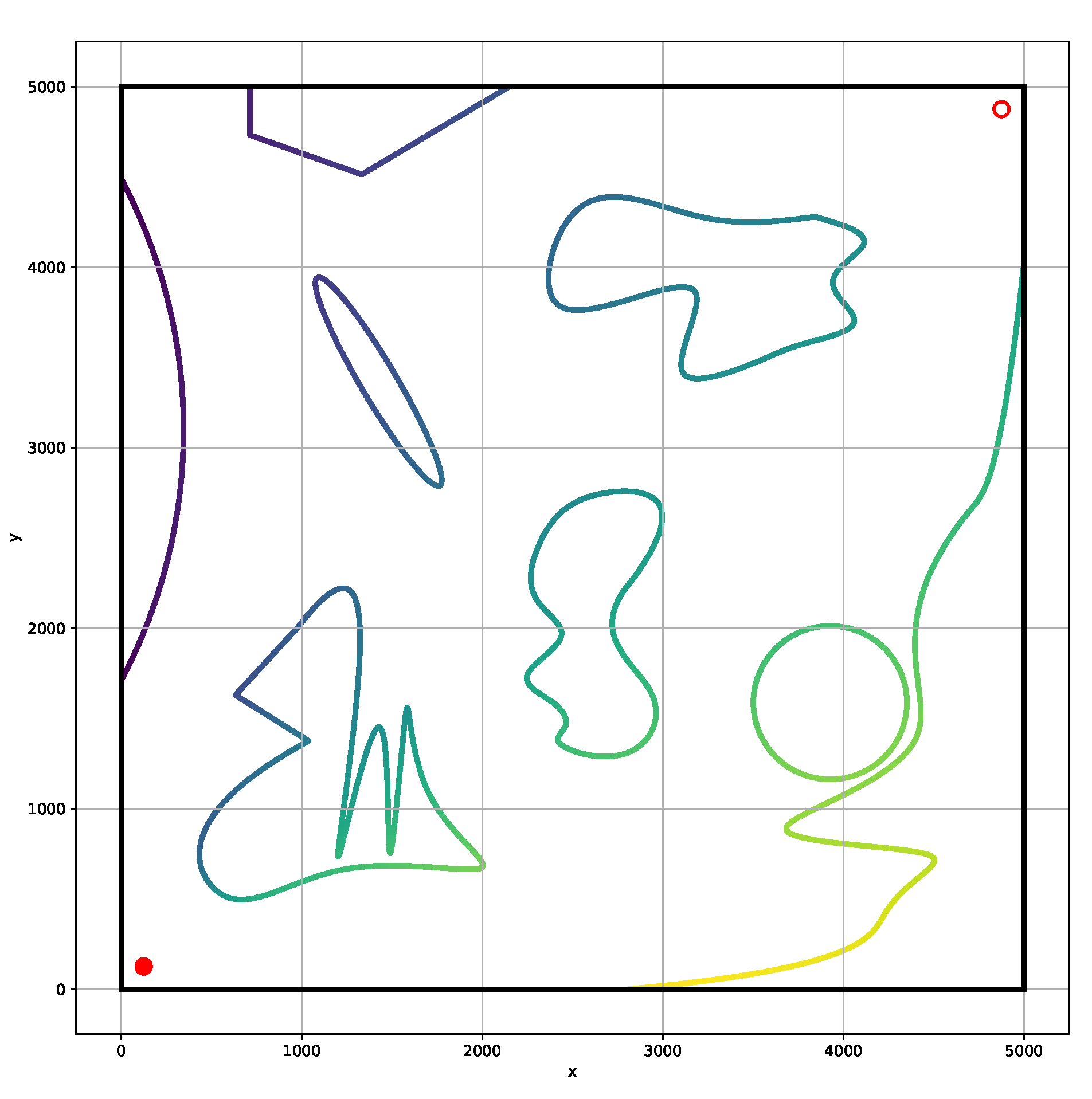
Smoothing is performed by including kinematics and curvature constraints on map obstacles. The final grid map is set to the resolution of 5 m/cell, as shown in Figure 3. The initial position is set at $(0.5,0.5)$, and the initial pose is defined as facing to the right, as shown in the red dot (lower left corner) in the figure. The target position is set at $(97.5,97.5)$, as shown in the red circle (upper right corner). The learning of the algorithm is mainly related to the a priori map and the starting point. The changing endpoint is always suitable for the cumulative error map to complete the learning and obtain the ideal path.

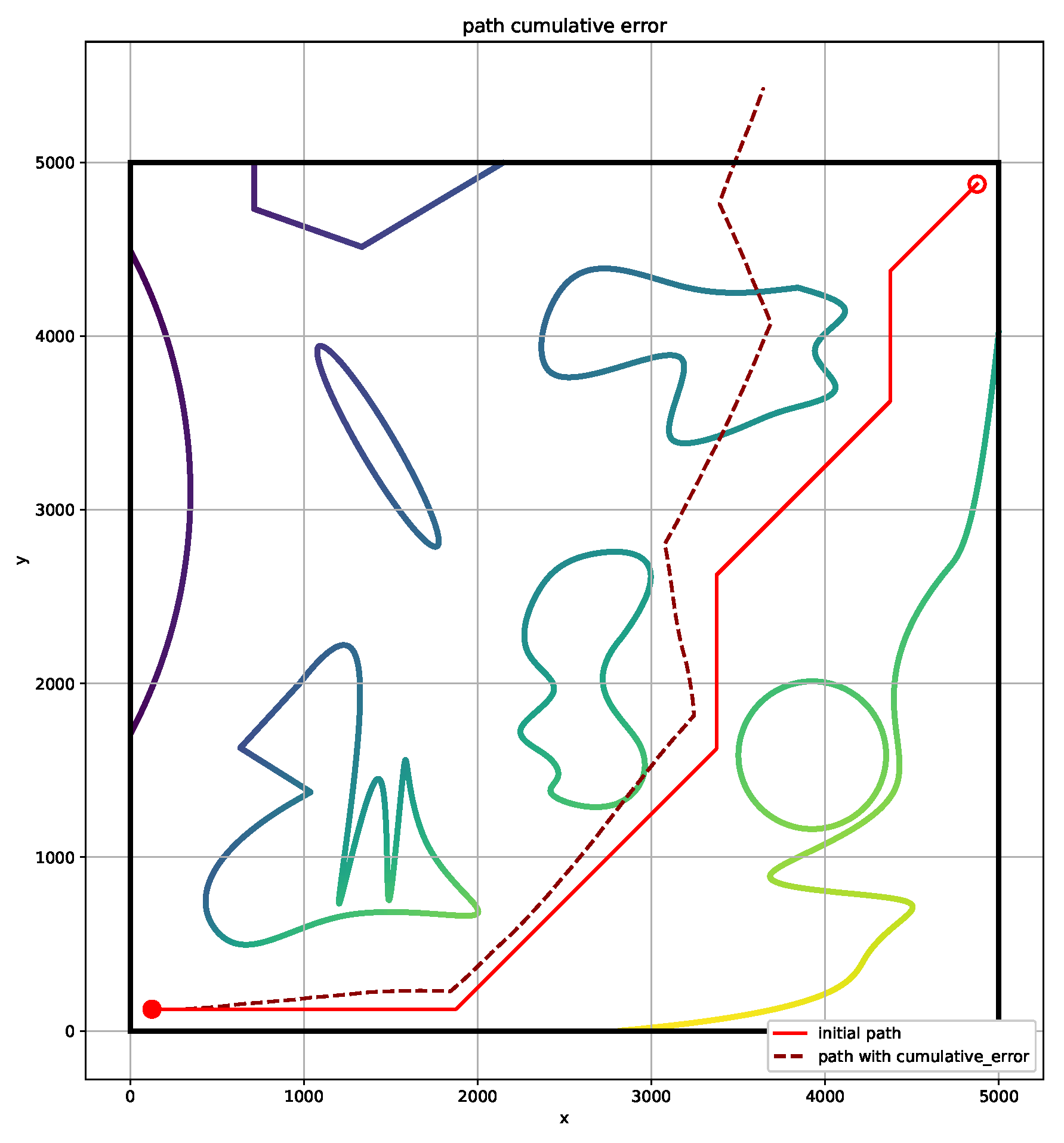
In general, the robot can accurately reach the end-point through the tracking process, with the help of high-precision GPS. In GPS-denied scenarios, considering the cumulative error originated from the noisy odometry sensors, with the distribution of $N(0,1)$ and $N(0,0.1)$ in both range and angular, respectively. As a result of the traditional reinforcement learning plan, the path can reach the end perfectly. At the moment, the reward/penalty is set to $1/-1$, and $\epsilon$ is set to $0.9$. However, considering the influence of the above-mentioned sensor noise, the actual path of the robot will deviate from original path and end-point to a large extent, as shown in Figure 4. The solid red path is originally planned and the red dotted path is one affected by the accumulated error. The cumulative error in paths with many turns is relatively large. In a scenario where the robot only relies on odometry, it is easy to deviate from the predetermined path.

Meanwhile, the proposed algorithm with reset parameters of rewards and punishments is adopted to obtain the ideal planning results. The specific parameter settings used in this paper are shown in

Table 1. Algorithm parameter settings.

States	Reward/Penalty	Value
Reach the boundary or obstacle	penalty	−1
Reach the end point	reward	100
Drive straight	penalty	−0.0001

, which does not imply optimal parameters. This paper has passed multiple tests and achieved a good simulation effect when $\epsilon =0.95$, and it is easier to get a convergence solution. Reinforcement learning algorithms based on probability selection have inconsistencies in results. This paper selects typical results as shown in Figure 5. The number of turns on planned path reduced, in which the cumulative error is significantly eliminated. The cumulative error is inevitable, whereas the localization error of the planning algorithm could be calculated effectively.

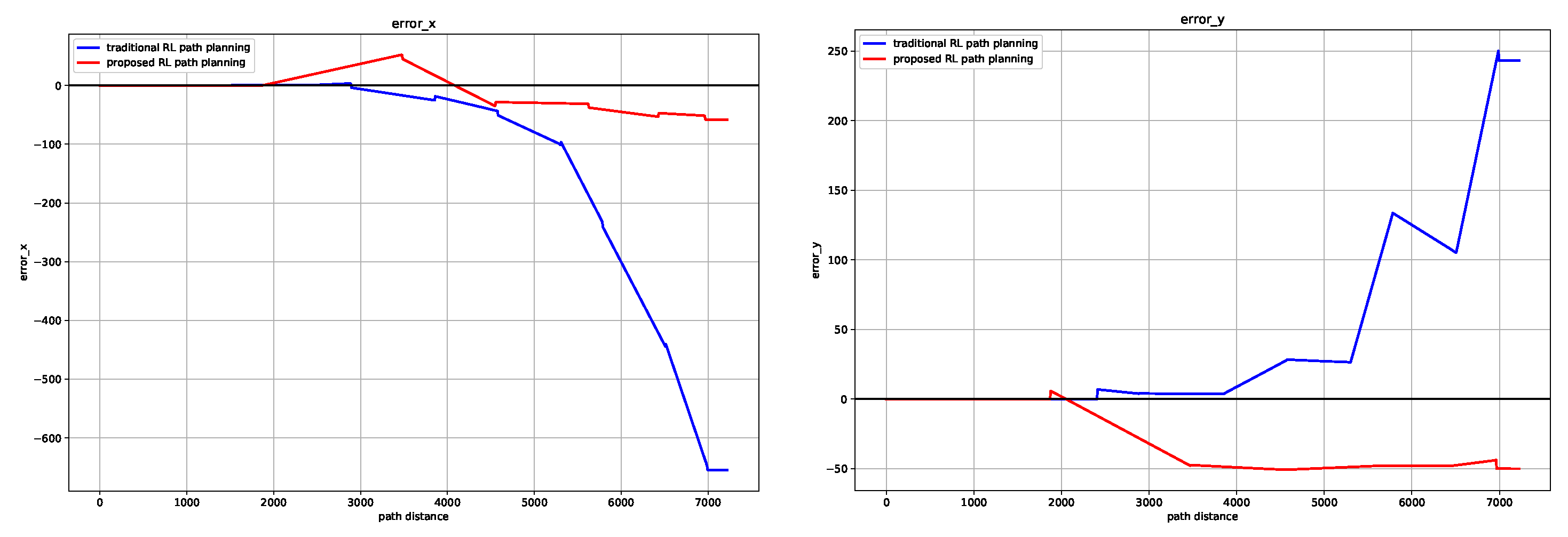
In the scene of constant robot speed, the cumulative error increases with time. Moreover, the cumulative error seems to increase significantly as the path turns increase. Compared with the traditional method, the proposed algorithm has a significant effect in reducing the cumulative error in the x and y directions (as shown in Figure 6), and the end-point of the tracking process is closer to the target point at the Euclidean distance. It is also verified from the application scenario that in the course of dead reckoning based on odometer, the positioning error caused by gyroscope error is greater than that caused by accelerometer error [26]. The reduction of accumulated error verifies the effectiveness of the algorithm.

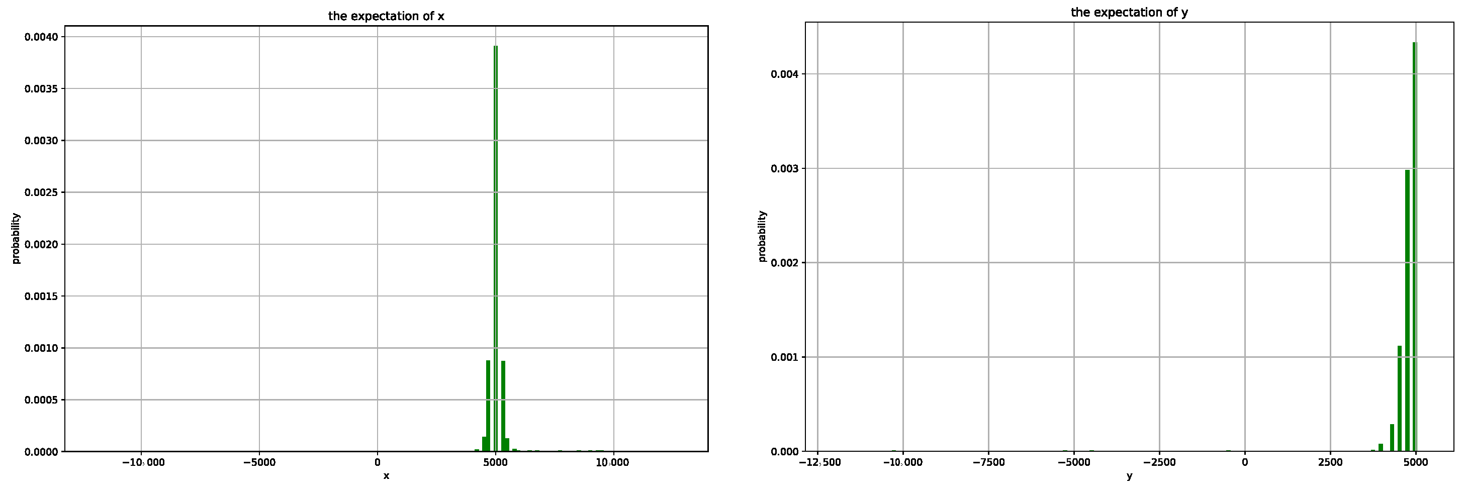
In the process of multiple iterations of planning, the expected value of each path in the x and y directions will fluctuate greatly, especially at the beginning of the algorithm. This is caused by the complicated path caused by probability in the early iteration process. After the algorithm converges, the expected values in the x and y directions remain around 4750 and 4750, as shown in Figure 7, which verifies the reliability of the algorithm.

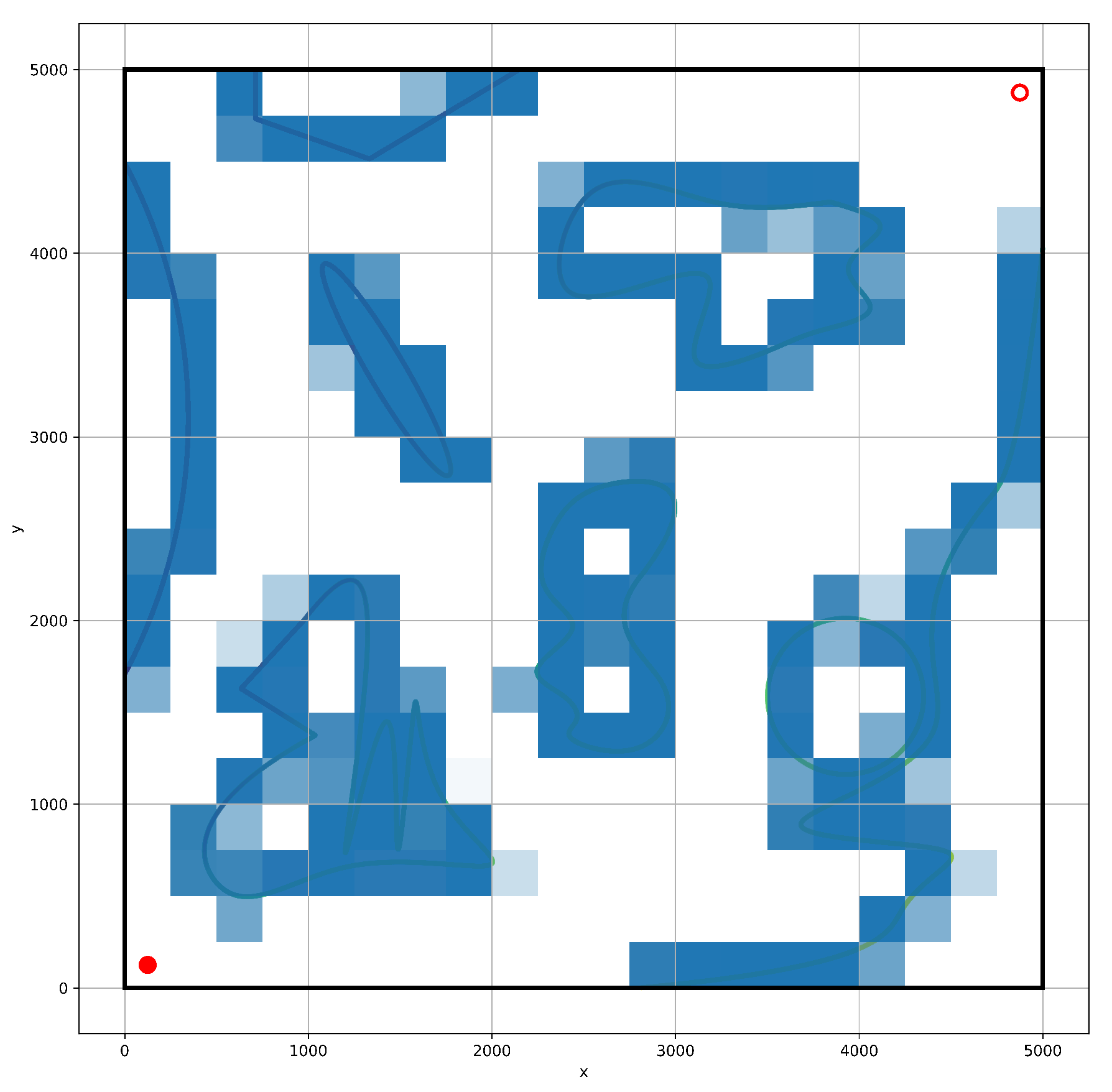
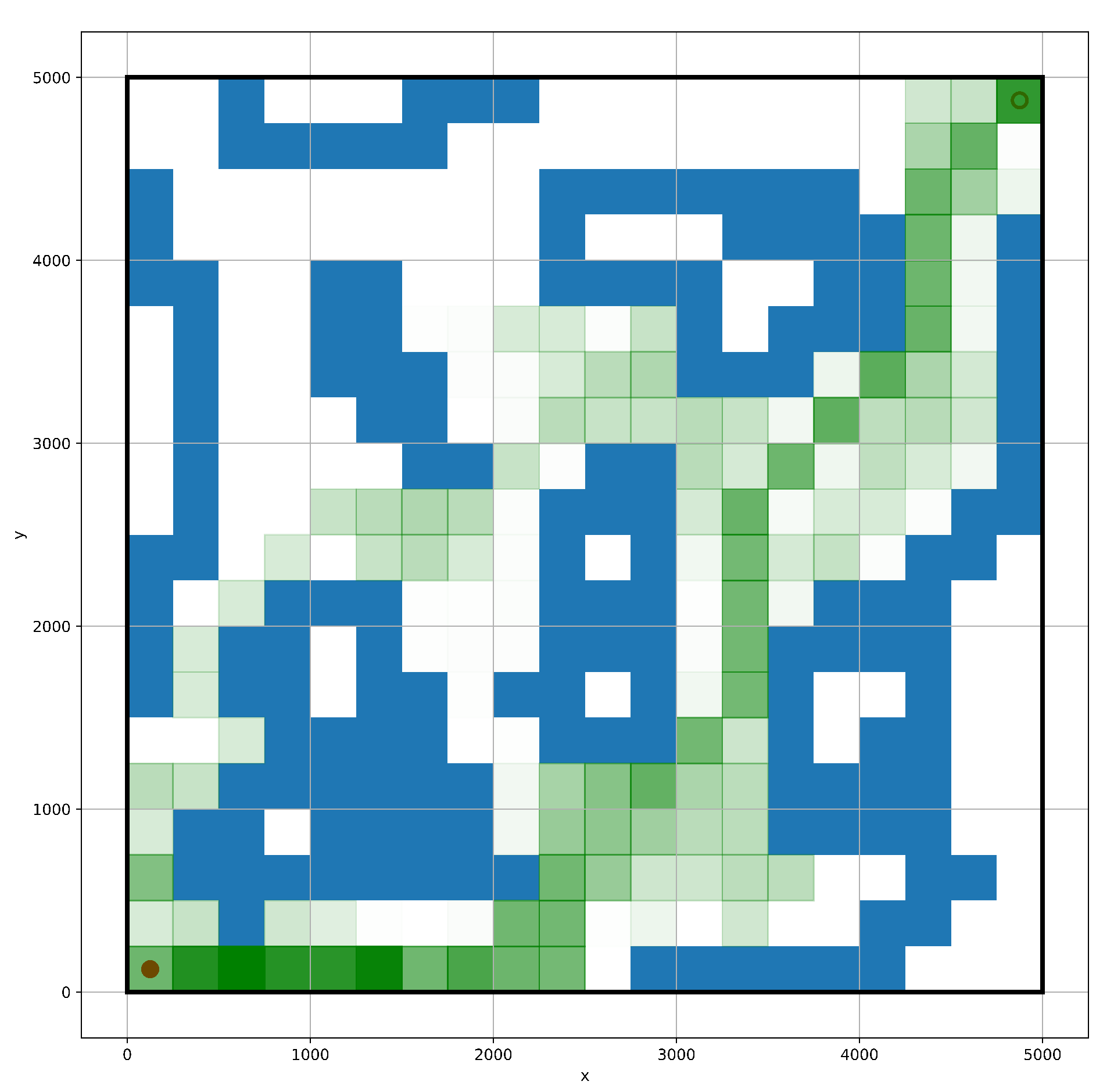
As the action selection is unknown, reinforcement learning algorithms will converge to different results, or even fail to converge to the best solution. In this paper, a heat map is made to visualize the iterative process of the algorithm, as shown in Figure 8. The agent reaches the area outside the optimal path many times, and finally, it converges to the vicinity of the optimal solution.

5. Conclusions

In GPS-denied scenarios, a path planning algorithm based on error estimation is proposed. Firstly, the cumulative error of the sensor noise is analyzed and the expectation and variance are described. Secondly, the reinforcement learning algorithm is utilized by considering the cumulative error during the planning process. Finally, the learning strategy is conducted to acquire an optimal path with noisy relative measurements. Simulation verifies that the proposed algorithm can effectively reduce the localization error of the robot in complex environments. The convergence results can be obtained through multiple learning processes, and the error expectation conforms to the theory, which shows the effectiveness and stability of the algorithm.