A New Model for Real-Time Prediction of Wellbore Stability Considering Elastic and Strength Anisotropy of Bedding Formation

Abstract

Severe wellbore stability issues were reported while drilling in laminated formation with weak planes such as beddings. To accurately determine the safe mud weight according to the changing environment is of primary importance for safety control of drilling. Considering both the elastic and strength anisotropy of bedding formation, a novel theoretical model is established and the stress and failure around wellbores are analyzed. The accuracy and applicability of the theoretical model is verified by in situ field data. For the purpose of fulfilling real-time prediction, the method flowchart of programming is also provided. The results show that the model built can be conveniently used to predict the stress distribution, failure area, and collapse and fracture pressure while drilling, and rather good predictions can be made compared to real field data. In addition, the inhomogeneity of in situ stress and elastic parameters affect the upper limit of the safe mud weight window (SMWW) greater than the lower limit. Negative SMWW may appear with the direction change of the wellbore or weak plane, especially when the azimuths of them change. As to the magnitude of SMWW, the anisotropic effects of Young’s modulus are greater than the Poisson’s ratio. The method established in this paper can greatly help with the precise prediction of wellbore stability as drilling proceeds in bedding formation.

1. Introduction

Bedding rocks such as shale are widely distributed in traditional energy deposition areas worldwide. According to the literature [1,2,3], shales constitute about 75% of the clastic sedimentary basins and about 90% of wellbore safety issues are related to the failure of shales. One of the most significant features about shale is the existence of bedding planes that originated from layered mineral sedimentation in history [4,5,6]. Therefore, the analysis of wellbore stability in bedding formations should fully consider the anisotropic effects that resulted from bedding planes.

Anisotropy, which is the intrinsic characteristic of bedding shales, has been widely researched in the literature. For example, lots of uniaxial and triaxial tests were carried out in the past to confirm that the compressive strength of bedding rocks is different when the angle between loading and bedding planes changes [7,8,9]. In addition, some researchers believe that the tensile strength of bedding rocks is also directional [10,11]. As to elastic parameters, some studies have proved that the anisotropies of Young’s modulus and Poisson’s ratio of bedding rocks are significant [12,13,14]. Ong [15] concluded that more than 30% of anisotropic rocks have an anisotropy ratio of 1.5 for Young’s modulus. Suarez-Rivera et al. [16] stated that the anisotropy ratio of Young’s modulus in tight gas shale can be up to 4.

Specialists have also made remarkable achievements related to wellbore stability in the past. Since Bradley [17] first established the systemic model of the hole-edge stress concentration problem, wellbore stability has been extensively studied under different conditions. Based on this basic model, the inclined and horizontal wellbore [18] and the failure criteria [19] are then analyzed. As to the multi-field coupling theory, Detournay and Cheng [20] built the earlier hydraulic-mechanical coupling model based on poroelastic theory to consider the infiltration effects of fluid. This model was further developed by Cui et al. [21] to incorporate the stability assessment of inclined wells. Based on this theory, Ding et al. [22] also considered the effects of anisotropic permeations that occurred around wellbores due to the existence of beddings. In addition, McTigue and Kurashige [23,24] established the thermal–hydraulic–mechanical coupling model to consider both the effects of thermal and hydraulic conduction around a wellbore. This model was further developed by many researchers [25,26,27] to consider the wider effects of non-isothermal condition, anisotropic thermal conduction, mechanical behavior of casing and cement sheath. As the drilling mud can be chemically-active and imbalance may exist between the drilling mud and rock formation, the chemical effects under this condition are investigated in the literature [28,29,30]. In addition, the plasticity effects were considered by Li et al. [31,32] to analyze the mechanical, seepage and temperature field around wellbores.

As to the effects of rock’s anisotropy on wellbore stability in bedding formation, the most common model only deals with strength anisotropy [33,34]. In this type of model, the bedding planes within rocks are believed to be weaker than the rock matrix and different strength criterion should be used to assess the failure of rock matrix and weak planes. For example, Deangeli and Omwanghe [35] applied this model to analyze how the orientation of weak planes and failure criterion affect wellbore stability in bedding formations. Ding et al. [18] built a model with generality to analyze inclined wellbores and compared it with the empirical model to verify its applicability in real field. The other type of model incorporates the effects of elastic anisotropy on the calculation of stresses around wellbores [36,37,38,39,40]. In this model, the elastic parameters such as Young’s modulus and Poisson’s ratio are assumed to have different values with regard to direction. Setiawan and Zimmerman [41] indicated that the stress concentration around wellbores when considering elastic anisotropy can be 25% higher than the isotropic condition. However, the model considering elastic anisotropy of rocks was not commonly applied when assessing wellbore stability in drilling practice as this model is rather complex and inconvenient to use.

Both the elastic and strength anisotropic effects of bedding rocks are significant according to the test results in the literature. It is quite necessary to establish the method that can be conveniently used to analyze the stresses and failures of bedding formation around wellbores. In this paper, a novel theoretical model of wellbore stability considering both strength and elastic anisotropy of rocks is established based on anisotropy theory, failure criteria and tensor transformations. The method flowchart for real-time calculation and analyzing of stresses and failures is provided, which can be easily applied as a framework of software programming and greatly increase the convenience of stability prediction while drilling in bedding formation. The accuracy and applicability of the model is verified by comparing the prediction results with the data in the real field. In addition, the influences of anisotropy, in situ stress and wellbore trajectory on the prediction results are also analyzed.

2. Stress Distribution around Wellbore in Anisotropic Bedding Rocks

The main problem to be solved in this paper is illustrated by Figure 1. The stresses around a deviated wellbore should be firstly calculated considering the elastic anisotropy of rocks. After that, transformation of stress and coefficient tensors should be carried out because different coordinate systems exist. Finally, the stability of the wellbore should be assessed considering the strength anisotropy of bedding formations. In addition, as the trajectory of wellbore and other factors may change with drilling proceeding to different depths, the real-time prediction of wellbore stability should be applicable.

2.1. Basic Equations for Drilling in Elastic Anisotropic Rocks

According to the elastic anisotropy theory and without the consideration of pore pressure, the general constitutive equations for the rocks around a wellbore can be expressed by Equation (1):

$$\left(\begin{array}{c}{\epsilon }_{xx}\\ {\epsilon }_{yy}\\ {\epsilon }_{zz}\\ {\gamma }_{yz}\\ {\gamma }_{xz}\\ {\gamma }_{xy}\end{array}\right)=\left(\begin{array}{cccccc}{a}_{11}& a_{12}& a_{13}& a_{14}& a_{15}& a_{16}\\ a_{21}& a_{22}& a_{23}& a_{24}& a_{25}& a_{26}\\ a_{31}& a_{32}& a_{33}& a_{34}& a_{35}& a_{36}\\ a_{41}& a_{42}& a_{43}& a_{44}& a_{45}& a_{46}\\ a_{51}& a_{52}& a_{53}& a_{54}& a_{55}& a_{56}\\ a_{61}& a_{62}& a_{63}& a_{64}& a_{65}& a_{66}\end{array}\right)\left(\begin{array}{c}{\sigma }_{xx}\\ {\sigma }_{yy}\\ {\sigma }_{zz}\\ {\tau }_{yz}\\ {\tau }_{xz}\\ {\tau }_{xy}\end{array}\right)$$

(1)

in which $a_{ij}$ are the components of the compliance tensor between stress and strain. As $a_{ij}$ have different values, we can see the anisotropic elastic property of rocks are fully considered here.

Considering the generalized plane strain conception built by Lekhnitskii-Amadei [36,37], one assumption is made that all the stresses, strain and displacements are identical within the plane vertical to the wellbore. According to this hypothesis, the governing equations are gradually introduced. First of all, the relation between strain and displacement can be written as:

$$\begin{array}{l}{\epsilon }_{xx}=\frac{\partial u}{\partial x}; {\epsilon }_{yy}=\frac{\partial v}{\partial y}; {\epsilon }_{zz}=0;\\ {\gamma }_{yz}=-\frac{\partial w}{\partial y}; {\gamma }_{zx}=-\frac{\partial w}{\partial x}; {\gamma }_{xy}=-\left(\frac{\partial u}{\partial y}+\frac{\partial v}{\partial x}\right)\end{array}$$

(2)

Then, the equilibrium equations can be expressed as

$$\begin{array}{l}\frac{\partial {\sigma }_{xx}}{\partial x}+\frac{\partial {\tau }_{xy}}{\partial y}=0\\ \frac{\partial {\tau }_{xy}}{\partial x}+\frac{\partial {\sigma }_{yy}}{\partial y}=0\\ \frac{\partial {\tau }_{xz}}{\partial x}+\frac{\partial {\tau }_{yz}}{\partial y}=0\end{array}$$

(3)

In addition, the compatibility equations can be expressed by Equation (4), as only three displacement components exist.

$$\begin{array}{l}\frac{{\partial }^2{\epsilon }_{xx}}{\partial y^2}+\frac{{\partial }^2{\epsilon }_{yy}}{\partial x^2}=\frac{{\partial }^2{\gamma }_{xy}}{\partial x\partial y}\\ \frac{\partial {\gamma }_{zx}}{\partial y}+\frac{\partial {\gamma }_{yz}}{\partial x}=0\end{array}$$

(4)

It is noted that ${\epsilon }_{zz}$ in Equation (1) is equal to zero according to the generalized plane strain assumption. Therefore, the axial stress can be expressed as

$${\sigma }_{zz}=-\frac{1}{a_{33}}(a_{31}{\sigma }_{xx}+a_{32}{\sigma }_{yy}+a_{34}{\tau }_{yz}+a_{35}{\tau }_{zx}+a_{36}{\tau }_{xy})$$

(5)

2.2. Solutions for Stress Distribution around Wellbore

The stresses in Equations (1) and (3) can be solved analytically. According to Amadei [37], two stress functions ($F(x,y)$, $\psi (x,y)$) are introduced to substitute the expression of stresses as:

$$\begin{array}{l}{\sigma }_{xx}=\frac{{\partial }^{2}F}{\partial y^2}; {\sigma }_{yy}=\frac{{\partial }^{2}F}{\partial x^2};\\ {\tau }_{xy}=-\frac{{\partial }^{2}F}{\partial x\partial y}; {\tau }_{xz}=-\frac{\partial \psi }{\partial y}; {\tau }_{Yz}=-\frac{\partial \psi }{\partial x}\end{array}$$

(6)

Then, the strain in Equation (1) can also be expressed by $F$ and $\psi$. After that, Equation (4) is converted to be the Beltrami–Michell equations as

$$l_4(\mu )l_2(\mu )-l_3{(\mu )}^2=0$$

(7)

in which $l_2$, $l_3$, $l_4$ are differential operators of different order:

$$\begin{array}{l}{l}_2(\mu )={\beta }_{44}\mu -2{\beta }_{45}\mu +{\beta }_{55}\mu \\ l_3(\mu )=-{\beta }_{24}\mu +({\beta }_{25}+{\beta }_{46})\mu -({\beta }_{14}+{\beta }_{56})\mu +{\beta }_{15}\mu \\ l_4(\mu )={\beta }_{22}\mu -2{\beta }_{26}\mu +(2{\beta }_{12}+{\beta }_{66})\mu -2{\beta }_{16}\mu +{\beta }_{11}\mu \end{array}$$

(8)

where ${\beta }_{ij}$ can be expressed by: ${\beta }_{ij}=a_{ij}-a_{i3}{a}_{j3}/a_{33}$. It is noted the six roots (${\mu }_i$, i = 1, 2, …, 6) of the above equation are all imaginary.

Define the spatial variable $z_i$ (i = 1, 2, 3) to be $z_i=x+{\mu }_{i}y$, then introduce the functions ${\varphi }_i(z_i)$ as:

$${\varphi }_1(z_1)=F_1{}^{\prime }(z_1); {\varphi }_2(z_2)=F_2{}^{\prime }(z_2); {\varphi }_3(z_3)=\frac{1}{{\lambda }_3}{F}_3{}^{\prime }(z_3)$$

(9)

where the ${\lambda }_i$ are expressed by:

$${\lambda }_1=-\frac{l_3({\mu }_1)}{l_2({\mu }_1)}; {\lambda }_2=-\frac{l_3({\mu }_2)}{l_2({\mu }_2)}; {\lambda }_3=-\frac{l_3({\mu }_3)}{l_4({\mu }_3)}$$

(10)

After that, the stress functions $F$ and $\psi$ can be generally expressed as:

$$\begin{array}{l}\frac{\partial F}{\partial x}=2\mathrm{Re}({\varphi }_1(z_1)+{\varphi }_2(z_2)+{\lambda }_3{\varphi }_3(z_3))\\ \frac{\partial F}{\partial y}=2\mathrm{Re}({\mu }_1{\varphi }_1(z_1)+{\mu }_2{\varphi }_2(z_2)+{\lambda }_3{\mu }_3{\varphi }_3(z_3))\\ \psi =2\mathrm{Re}({\lambda }_1{\varphi }_1(z_1)+{\lambda }_2{\varphi }_2(z_2)+{\varphi }_3(z_3))\end{array}$$

(11)

in which Re represents the real part of the expression. Once $F$ and $\psi$ are obtained, the stresses around the wellbore can be shown as:

$$\begin{array}{l}{\sigma }_{xx}=2\mathrm{Re}({\mu }_1{}^2{\varphi }_1{}^{\prime }(z_1)+{\mu }_2{}^2{\varphi }_2{}^{\prime }(z_2)+{\lambda }_3{\mu }_3{}^2{\varphi }_3{}^{\prime }(z_3))\\ {\sigma }_{yy}=2\mathrm{Re}({\varphi }_1{}^{\prime }(z_1)+{\varphi }_2{}^{\prime }(z_2)+{\lambda }_3{\varphi }_3{}^{\prime }(z_3))\\ {\tau }_{yz}=-2\mathrm{Re}({\lambda }_1{\varphi }_1{}^{\prime }(z_1)+{\lambda }_2{\varphi }_2{}^{\prime }(z_2)+{\varphi }_3{}^{\prime }(z_3))\\ {\tau }_{zx}=2\mathrm{Re}({\lambda }_1{\mu }_1{\varphi }_1{}^{\prime }(z_1)+{\lambda }_2{\mu }_2{\varphi }_2{}^{\prime }(z_2)+{\mu }_3{\varphi }_3{}^{\prime }(z_3))\\ {\tau }_{xy}=-2\mathrm{Re}({\mu }_1{\varphi }_1{}^{\prime }(z_1)+{\mu }_2{\varphi }_2{}^{\prime }(z_2)+{\lambda }_3{\mu }_3{\varphi }_3{}^{\prime }(z_3))\end{array}$$

(12)

To obtain the solution of ${\varphi }_i{}^{\prime }(z_i)$ (i = 1, 2, 3) in real field, the boundary conditions around the wellbore should be considered, which include the in situ stress acting in far-field and the mud pressure acting within the wellbore. These two boundary conditions can be expressed by Equations (13) and (14).

$$\begin{array}{l}{\sigma }_{xx}\cos \theta +{\tau }_{xy}\sin \theta =-({\sigma }_{xx,0}\cos \theta +{\tau }_{xy,0}\sin \theta )\\ {\tau }_{xy}\cos \theta +{\sigma }_{yy}\sin \theta =-({\tau }_{xy,0}\cos \theta +{\sigma }_{yy,0}\sin \theta )\\ {\tau }_{zx}\cos \theta +{\tau }_{yz}\sin \theta =-({\tau }_{zx,0}\cos \theta +{\tau }_{yz,0}\sin \theta )\end{array}$$

(13)

$$\begin{array}{l}{\sigma }_{xx}\cos \theta +{\tau }_{xy}\sin \theta =p_w\cos \theta \\ {\tau }_{xy}\cos \theta +{\sigma }_{yy}\sin \theta =p_w\sin \theta \\ {\tau }_{zx}\cos \theta +{\tau }_{yz}\sin \theta =0\end{array}$$

(14)

in which ${\sigma }_{kl,0}$ represent the components of in situ stress, p_w represents the mud pressure within the wellbore, $\theta$ represents the hoop angle around wellbore. Combining Equations (12)–(14), the ${\varphi }_i{}^{\prime }(z_i)$ can be solved as:

$$\begin{array}{cc}\hfill & {{\varphi }_1}^{\prime }\left(z_1\right)={\gamma }_1[({\mu }_3{\lambda }_2{\lambda }_3-{\mu }_2)({\sigma }_{yy,0}-i{\tau }_{xy,0}-p_w)+({\lambda }_2{\lambda }_3-1)({\tau }_{xy,0}-i{\sigma }_{xx,0}+i{p}_w)\hfill \\ \hfill & +{\lambda }_3({\mu }_3-{\mu }_2)({\tau }_{yz,0}-i{\tau }_{xz,0})]\hfill \\ \hfill & {{\varphi }_2}^{\prime }\left(z_2\right)={\gamma }_2[-({\mu }_3{\lambda }_1{\lambda }_3-{\mu }_1)({\sigma }_{yy,0}-i{\tau }_{xy,0}-p_w)+(1-{\lambda }_2{\lambda }_3)({\tau }_{xy,0}-i{\sigma }_{xx,0}+i{p}_w)\hfill \\ \hfill & +{\lambda }_3({\mu }_1-{\mu }_3)({\tau }_{yz,0}-i{\tau }_{xz,0})]\hfill \\ \hfill & {{\varphi }_3}^{\prime }\left(z_3\right)={\gamma }_3[({\mu }_2{\lambda }_1-{\mu }_1{\lambda }_2)({\sigma }_{yy,0}-i{\tau }_{xy,0}-p_w)+({\lambda }_1-{\lambda }_2)({\tau }_{xy,0}-i{\sigma }_{xx,0}+i{p}_w)\hfill \\ \hfill & +({\mu }_2-{\mu }_1)({\tau }_{yz,0}-i{\tau }_{xz,0})]\hfill \end{array}$$

(15)

with

$$\begin{array}{l}{\gamma }_j={\left(-2\Delta p_j\sqrt{{\left(\frac{z_j}{a}\right)}^2-1-{\mu }_j{}^2}\right)}^{-1},\hspace{1em}j=1,2,3\\ p_j=\frac{\frac{z_j}{a}+\sqrt{{\left(\frac{z_j}{a}\right)}^2-1-{\mu }_j{}^2}}{1-i{\mu }_j},\hspace{1em}j=1,2,3\\ \Delta ={\mu }_2-{\mu }_1+{\lambda }_2{\lambda }_3({\mu }_1-{\mu }_3)+{\lambda }_1{\lambda }_3({\mu }_3-{\mu }_2)\end{array}$$

(16)

where $a$ is the wellbore radius.

3. Failure Criteria Considering Strength Anisotropy of Rocks around Wellbore

Generally, the safe wellbore pressure window is determined by collapse and fracture failure criteria of surrounding rocks. When the mud pressure within the wellbore is low enough, collapse failure of rocks may occur on the wellbore wall. Otherwise, if the mud pressure is high enough, fracture failure of rocks will happen. Therefore, it is critical to predict the safe wellbore pressure window precisely to maintain stable drilling, especially when the orientation of the wellbore varies with depth. In laminated formation such as shale, the anisotropic strength of rocks should also be taken into consideration.

3.1. Collapse Failure of Rock Matrix

Many compressive failure criteria have been applied to assess the strength of intact rocks in the literature, for example, the Mohr–Coulomb criterion, the Drucker–Prager criterion, the Mogi–Coulomb criterion, the Hoek–Brown, etc. According to the illustrations of Al-Ajmi and Zimmerman [42], the Mohr–Coulomb criterion does not consider the influences of the intermediate stress while the D–P criterion exaggerates the strengthening effects; in contrast, the Mogi–Coulomb criterion can predict the strength of brittle rocks pretty well. This conclusion was further verified by the experiments and in situ studies of Zhang et al. [43] and Gholami et al. [44]. The form of this criterion is expressed as:

$${\tau }_{oct}=a+b{\sigma }_{m,2}$$

(17)

with

$$\begin{array}{l}{\tau }_{oct}=\frac{1}{3}\sqrt{{({\sigma }_1-{\sigma }_2)}^2+{({\sigma }_2-{\sigma }_3)}^2+{({\sigma }_1-{\sigma }_3)}^2}\\ {\sigma }_{m,2}=\frac{{\sigma }_1+{\sigma }_3}{2}\\ a=\frac{2\sqrt{2}}{3}{c}_m\cos {\phi }_m\\ b=\frac{2\sqrt{2}}{3}\sin {\phi }_m\end{array}$$

(18)

where $c_m$ and ${\phi }_m$ are the cohesion and friction angle of rock matrix, respectively. The effects of intermediate principal stress (${\sigma }_2$) are considered in the Mogi-C criterion. It should be noted that the principal stresses in Equation (18) are effective stresses therefore the influence of pore pressure on failure of rocks can be considered. This also applies to the subsequent failure criteria.

3.2. Collapse Failure of Weak Planes

As strength weakening effects of anisotropic rocks been verified by many experiments [7,8,9], the weak plane Mohr–Coulomb criterion [45] is applied to predict failure of weak planes:

$$\tau =c_w+{\sigma }_n\tan {\phi }_w$$

(19)

in which $c_w$ and ${\phi }_w$ are the cohesion and internal friction angle of weak planes, respectively.

3.3. Fracture Failure of Rocks

Fracture of rocks around wellbores is caused by tensile failure, therefore, a simple tensile strength criterion could be used:

$${\sigma }_3<S_t$$

(20)

in which ${\sigma }_3$ is the minimum principal stress around wellbore and $S_t$ is the tensile strength of rocks. If the anisotropy of tensile strength for bedding rocks is considered, Ding et al. [18] analyzed the related influences on wellbore stability, but this is not the focus here and thus is not discussed.

4. Real-Time Prediction of Safe Drilling Mud Weight in Anisotropic Bedding Formation

4.1. Tensor Transformations between Different Coordinate Systems

4.1.1. Stress Tensor Transformation

As shown by Figure 2, if we assume the in situ stress coordinate system is in accordance with the global coordinate system, then three coordinate systems (named the global coordinate system (GCS), the wellbore coordinate system (WCS) and the weak-plane coordinate system (WPCS)) can be built for further analyses. It is noted with the help of computer programing, tensor transformations can be conveniently realized between different coordinate systems. After that, the change of wellbore trajectory and the influences of inclined weak planes can be included in the real-time analysis processing.

According to geometric relation and the angle definitions of Figure 2, the transformation matrix between GCS and WCS (GCS and WPCS) can be written by $R_1$ ($R_2$) as:

$$R_1=\left[\begin{array}{ccc}\cos {\alpha }_1\cos {\beta }_1& \sin {\alpha }_1\cos {\beta }_1& -\sin {\beta }_1\\ -\sin {\alpha }_1& \cos {\alpha }_1& 0\\ \cos {\alpha }_1\sin {\beta }_1& \sin {\alpha }_1\sin {\beta }_1& \cos {\beta }_1\end{array}\right]$$

(21)

$$R_2=\left[\begin{array}{ccc}\cos {\alpha }_2\cos {\beta }_2& \sin {\alpha }_2\cos {\beta }_2& -\sin {\beta }_2\\ -\sin {\alpha }_2& \cos {\alpha }_2& 0\\ \cos {\alpha }_2\sin {\beta }_2& \sin {\alpha }_2\sin {\beta }_2& \cos {\beta }_2\end{array}\right]$$

(22)

As $R_1$ and $R_2$ are orthogonal, a stress tensor ${\sigma }_g$ (3 × 3 matrix) under GCS can be transformed to WCS by:

$${\sigma }_b=R_1 {\sigma }_g R_1^T$$

(23)

Furthermore, if the stress solution (${\sigma }_{sol}$) in Equation (12) is obtained, then this solution can be expressed under WPCS by:

$${\sigma }_{sol,w}=R_2 R_1^T {\sigma }_{sol} R_1 R_2^T$$

(24)

After that, the $\tau$ and ${\sigma }_n$ in Equation (19) can be obtained by

$$\begin{array}{l}\tau =\sqrt{{\tau }_{xz}^2+{\tau }_{yz}^2}\\ {\sigma }_n={\sigma }_{zz}\end{array}$$

(25)

where the ${\sigma }_{zz}, {\tau }_{xz}, {\tau }_{yz}$ are the components of ${\sigma }_{sol,w}$.

In addition to that, for the most general condition when the in situ stress coordinate system (ICS) is not in accordance with the GCS, the transformation between ICS and GCS was built by Ding et al. [18] using the following matrix $R_3$:

$$R_3=\left[\begin{array}{ccc}\cos {\alpha }_3\cos {\beta }_3& \sin {\alpha }_3\cos {\beta }_3& -\sin {\beta }_3\\ \cos {\alpha }_3\sin {\beta }_3\sin {\gamma }_3-\sin \alpha \cos {\gamma }_3& \sin {\alpha }_3\sin {\beta }_3\sin {\gamma }_3+\cos {\alpha }_3\cos {\gamma }_3& \cos {\beta }_3\sin {\gamma }_3\\ \cos {\alpha }_3\sin {\beta }_3\cos {\gamma }_3-\sin {\alpha }_3\sin {\gamma }_3& \sin {\alpha }_3\sin {\beta }_3\cos {\gamma }_3+\cos {\alpha }_3\sin {\gamma }_3& \cos {\beta }_3\cos {\gamma }_3\end{array}\right]$$

(26)

4.1.2. Compliance Tensor Transformation

It is noted that the compliance tensor in Equation (1) is actually expressed under WCS. However, the general compliance tensor for rocks with weak planes (transversely isotropic rocks) can be expressed under WPCS by:

$$A=\left(\begin{array}{cccccc}\frac{1}{E_h}& -\frac{v_h}{E_h}& -\frac{v_v}{E_v}& 0& 0& 0\\ & \frac{1}{E_h}& -\frac{v_v}{E_v}& 0& 0& 0\\ & & \frac{1}{E_v}& 0& 0& 0\\ & & & \frac{1}{G_v}& 0& 0\\ & & & & \frac{1}{G_v}& 0\\ & & & & & \frac{2(1+v_h)}{E_h}\end{array}\right)$$

(27)

where the subscript v and h denote the normal and in-plane direction of the weak plane, respectively.

If the Equations (21) and (22) are written to be:

$$R_i=\left[\begin{array}{ccc}{l}_1& m_1& n_1\\ l_2& m_2& n_2\\ l_3& m_3& n_3\end{array}\right], \mathrm{i}=1, 2$$

(28)

then according to the geometric relation of different coordinate systems, the compliance tensor $A_b$ under WCS can be obtained by the following transformation relation:

$$A_b=T_{\epsilon }{}_{,1} {[T_{\sigma ,}{}_2]}^T A T_{\sigma }{}_{,2} {[T_{\epsilon ,1}]}^T$$

(29)

where the $T_{\sigma ,i}$ and $T_{\epsilon ,i}$ are 6 × 6 Bond transformation matrices that can be expressed by:

$${\mathbf{T}}_{\mathbf{\sigma },\mathbf{i}}=\left(\begin{array}{cccccc}{l_1}^2& {m_1}^2& {n_1}^2& 2m_1{n}_1& 2n_1{l}_1& 2l_1{m}_1\\ {l_2}^2& {m_2}^2& {n_2}^2& 2m_2{n}_2& 2n_2{l}_2& 2l_2{m}_2\\ {l_3}^2& {m_3}^2& {n_3}^2& 2m_3{n}_3& 2n_3{l}_3& 2l_3{m}_3\\ l_2{l}_3& m_2{m}_3& n_2{n}_3& m_2{n}_3+m_3{n}_2& n_2{l}_3+n_3{l}_2& l_2{m}_3+l_3{m}_2\\ l_3{l}_1& m_3{m}_1& n_3{n}_1& m_1{n}_3+m_3{n}_1& n_1{l}_3+n_3{l}_1& l_1{m}_3+l_3{m}_1\\ l_1{l}_2& m_1{m}_2& n_1{n}_2& m_1{n}_2+m_2{n}_1& n_1{l}_2+n_2{l}_1& l_1{m}_2+l_2{m}_1\end{array}\right), i=1,2$$

(30)

$${\mathbf{T}}_{\mathbf{\epsilon },\mathbf{i}}=\left(\begin{array}{cccccc}{l_1}^2& {m_1}^2& {n_1}^2& m_1{n}_1& n_1{l}_1& l_1{m}_1\\ {l_2}^2& {m_2}^2& {n_2}^2& m_2{n}_2& n_2{l}_2& l_2{m}_2\\ {l_3}^2& {m_3}^2& {n_3}^2& m_3{n}_3& n_3{l}_3& l_3{m}_3\\ 2l_2{l}_3& 2m_2{m}_3& 2n_2{n}_3& m_2{n}_3+m_3{n}_2& n_2{l}_3+n_3{l}_2& l_2{m}_3+l_3{m}_2\\ 2l_3{l}_1& 2m_3{m}_1& 2n_3{n}_1& m_1{n}_3+m_3{n}_1& n_1{l}_3+n_3{l}_1& l_1{m}_3+l_3{m}_1\\ 2l_1{l}_2& 2m_1{m}_2& 2n_1{n}_2& m_1{n}_2+m_2{n}_1& n_1{l}_2+n_2{l}_1& l_1{m}_2+l_2{m}_1\end{array}\right), i=1,2$$

(31)

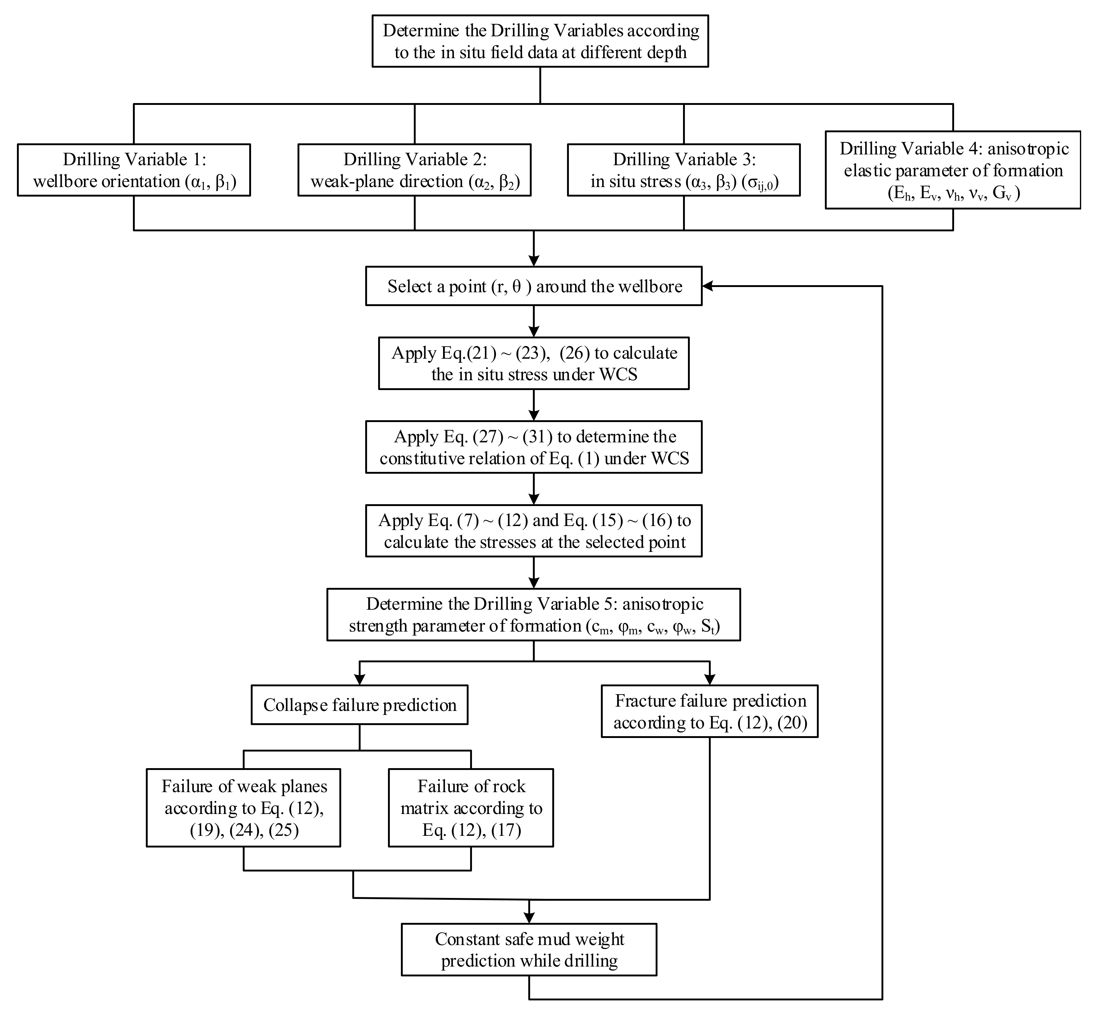
4.2. Flowchart for Programing

The procedures of real-time prediction of safe mud weight can be shown by the flowchart in Figure 3. The drilling variables can be divided into five categories, which are the directions of wellbore and weak planes, in situ stress, and the elastic and strength anisotropic parameters of rocks. Actually, it is known that the information about in situ stress, bedding planes and rock parameters cannot be obtained while drilling based on the current technology. Only the wellbore trajectory (azimuth and inclination) information can be obtained in real-time by downhole measuring tools. Therefore, this real-time prediction model can now apply to the situation when earlier drillings have been implemented in the same area so that the information about in situ stress, bedding planes and rock parameters have already been obtained. All these variables, whether detected before or current, may be different with depth. Then, the real-time prediction of stress, failure and safe mud weight can be conveniently achieved by using software programing following the scheme in Figure 3.

5. Calculation Results and Analyses of the Case in Real Field

To meet the most general situation, the model built and the method developed in this paper should fully consider the factors of the in situ stress, orientations of wellbore and weak planes, strength and elastic parameters of anisotropic rocks, etc. In this section, part of the in situ field data in the Boulder area collected by McLellan and Cormier [46] are applied for calculation and analysis. The Boulder wells were directionally drilled to targets in the gas producing formations. In this region the geology consists of a series of stacked thrust sheets, with multiple faulted imbricates offsetting the weaker parts of the formations. Laminated rocks such as shales, interbedded sandstones and siltstones are widely spread in this area. Significant directional drilling efforts were made to ensure penetration of the formation to the target. It is reported that severe wellbore stability problems occurred in this area during the drilling process. The basic parameters in this area are listed in

Table 1. In situ field data in the Boulder area of Northeastern British Columbia [46].

Item	Value/Unit
Wellbore depth	2100 m
$\mathrm{Wellbore} \mathrm{radius} a$	0.1 m
$\mathrm{Maximum} \mathrm{horizontal} \mathrm{in} \mathrm{situ} \mathrm{stress} \mathrm{gradient} {\sigma }_H$	28 MPa/km
$\mathrm{Minimum} \mathrm{horizontal} \mathrm{in} \mathrm{situ} \mathrm{stress} \mathrm{gradient} {\sigma }_h$	15 MPa/km
$\mathrm{Overburden} \mathrm{in} \mathrm{situ} \mathrm{stress} \mathrm{gradient} {\sigma }_v$	30 MPa/km
$\mathrm{Pore} \mathrm{pressure} \mathrm{gradient} p_0$	9.8 MPa/km
$\mathrm{Drilling} \mathrm{mud} \mathrm{weight} \rho$	1.02 g/cm3
Orientation of in situ stress	${\alpha }_3=50°, {\beta }_3=0°, {\gamma }_3$ = 0°
Orientation of wellbore	${\alpha }_1=110°, {\beta }_1$ = 50°
Orientation of bedding planes	${\alpha }_2=205°, {\beta }_2$ = 60°
Horizontal Young’s modulus of rocks $E_h$	31,170 MPa
Vertical Young’s modulus of rocks $E_v$	15,420 MPa
Horizontal Poisson’s ratio of rocks ${\nu }_h$	0.079
Vertical Poisson’s ratio of rocks ${\nu }_v$	0.3
$\mathrm{Vertical} \mathrm{Shear} \mathrm{modulus} \mathrm{of} \mathrm{rocks} G_v$	7050 MPa
Biot’s effective stress coefficient $\alpha$	1
$\mathrm{Cohesion} \mathrm{of} \mathrm{rock} \mathrm{matrix} c_m$	4.3 MPa
$\mathrm{Friction} \mathrm{angle} \mathrm{of} \mathrm{rock} \mathrm{matrix} {\phi }_m$	30°
$\mathrm{Cohesion} \mathrm{of} \mathrm{weak} \mathrm{planes} c_w$	0.1 MPa
$\mathrm{Friction} \mathrm{angle} \mathrm{of} \mathrm{weak} \mathrm{planes} {\phi }_w$	25°
$\mathrm{Tensile} \mathrm{strength} \mathrm{of} \mathrm{rocks} S_t$	0 MPa

The elastic parameters of anisotropic rocks are from Shale E5 [13].

. It is noted that a normal-faulting in situ stress regime (${\sigma }_v>{\sigma }_H>{\sigma }_h$) is assumed here and the orientations of the in situ stress, wellbore and beddings are quite random.

5.1. Calculation Results of the Case with Generality

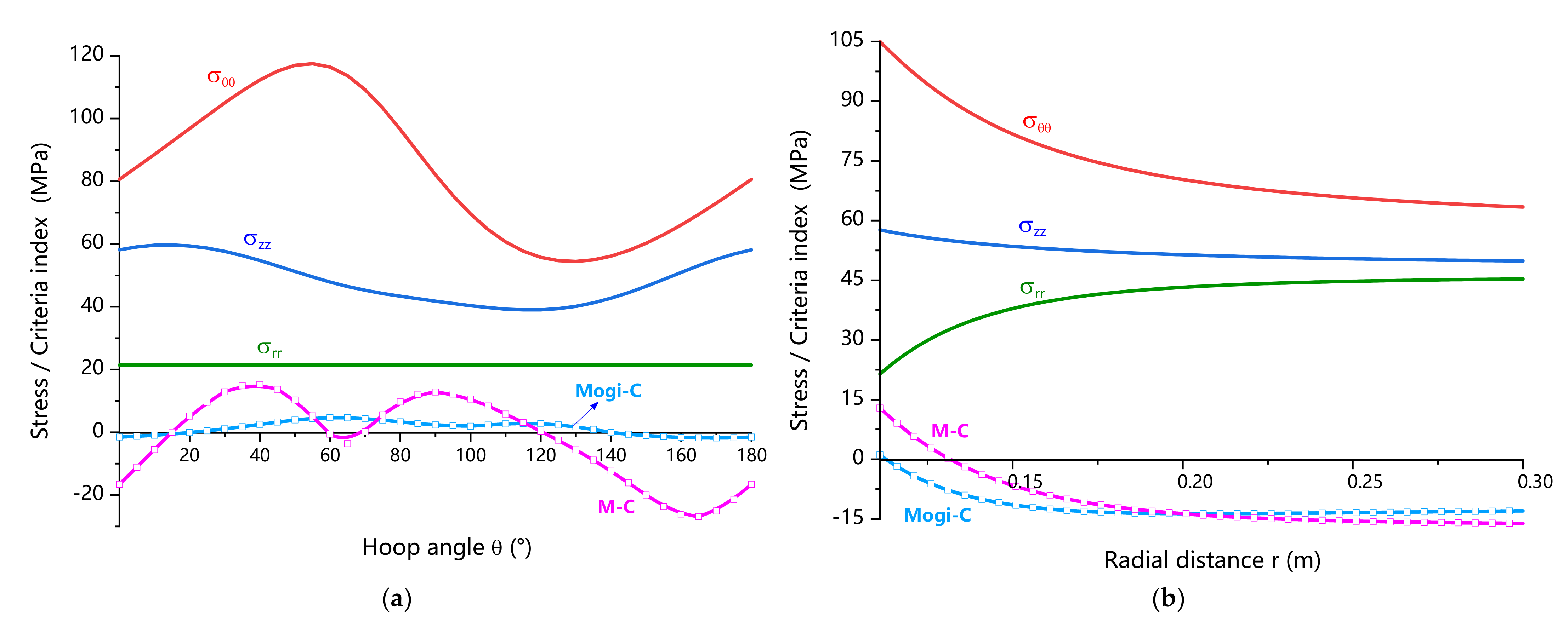
5.1.1. Stress Distribution around the Wellbore

Following the flowchart in Figure 3, the first step for wellbore stability analysis is the calculation of stress distribution around the wellbore. In Figure 4, the stress distributions around the wellbore (Table 1) in the radial and the hoop direction are all illustrated. In addition, two criteria indexes are defined by Equation (32) based on Equation (17) and Equation (19) and the results also indicated in Figure 4.

$$\begin{array}{l}Index \mathrm{of}\hspace{1em}Mogi-C={\tau }_{oct}-a-b{\sigma }_{m,2}\\ Index \mathrm{of} M-C=\tau -c_w-{\sigma }_n\tan {\phi }_w\end{array}$$

(32)

From the definition, it is known the positive value of the criteria indexes means failure while the negative value means stability. From Figure 4a, it is seen that the hoop (${\sigma }_{\theta \theta }$) and axial stress (${\sigma }_{zz}$) change regularly in the circumferential direction around the wellbore while the radial stress (${\sigma }_{rr}$) is constant. This is because the radial distance of r = a is selected here, thus the ${\sigma }_{rr}$ is equal to mud pressure (p_w). In addition, positive values of Mogi–C and M–C appear in the hoop direction, which means failure of both rock matrix and weak planes occurs on the wellbore wall. In Figure 4b, the hoop angle of $\theta$ = 30° is selected for the calculation of stresses in the radial direction. From Figure 4b, it is seen that a great change of stresses happens near the wellbore while little change happens far away from the hole. In addition, according to the results of criteria indexes, failure of rocks only happens within an area near the hole.

5.1.2. Failure Area around the Wellbore

The failure area around wellbore can also be conveniently calculated using the developed model. With the help of software programming, the stability of every point ($r=a+i\ast \Delta r$, $\theta =i\ast \Delta \theta$) around the wellbore can be evaluated efficiently. Figure 5 shows the results of failure area calculated based on rock matrix and weak planes, respectively. It is seen that the failure area is calculated considering the failure of bedding planes are much larger than that of rock matrix. This is because the strength of bedding planes is much weaker than that of rock matrix (Table 1). In addition, in Figure 5a, failures extend in two opposite directions while the failure area in Figure 5b is in the shape of a “four-leaf-clover”. This phenomenon is also proved by Lee et al. [4].

5.1.3. Collapse Stress and Fracture Stress

The most critical results of model prediction for guiding drilling practice may be the calculation of collapse pressure and fracture pressure, which defined the lower and upper limits of permitted wellbore pressure. To calculate the collapse and fracture pressure, every point around the wellbore ($r=a+i\ast \Delta r$, $\theta =i\ast \Delta \theta$) can be selected successively, and the criteria indexes can be calculated with the change of wellbore pressure (p_w). The change of these indexes from negative to positive (positive to negative) means collapse (fracture) failure happens.

Because of symmetry, only the results of the points with $\theta$ = 0~180° are shown in Figure 6. It is seen for every point around the wellbore that the critical value of p_w can be determined by collapse or fracture failure of rocks. These critical values constitute a curve that will determine the final collapse or fracture pressure. It is easy to understand that to maintain a stable wellbore, the maximum value of the collapse curve will be the collapse pressure while the minimum value of the fracture curve will be the fracture pressure. From Figure 6, it is seen that the collapse pressure decided by failure of weak planes is higher than that decided by failure of rock matrix. Consequently, the safe wellbore pressure window (${\Delta }_1$) decided by failure of weak planes is narrower than that decided by failure of rock matrix (${\Delta }_2$). This means considering the failure of weak planes is quite critical in drilling engineering when bedding formations are encountered.

5.2. Factors Influencing the Safe Mud Weight Window

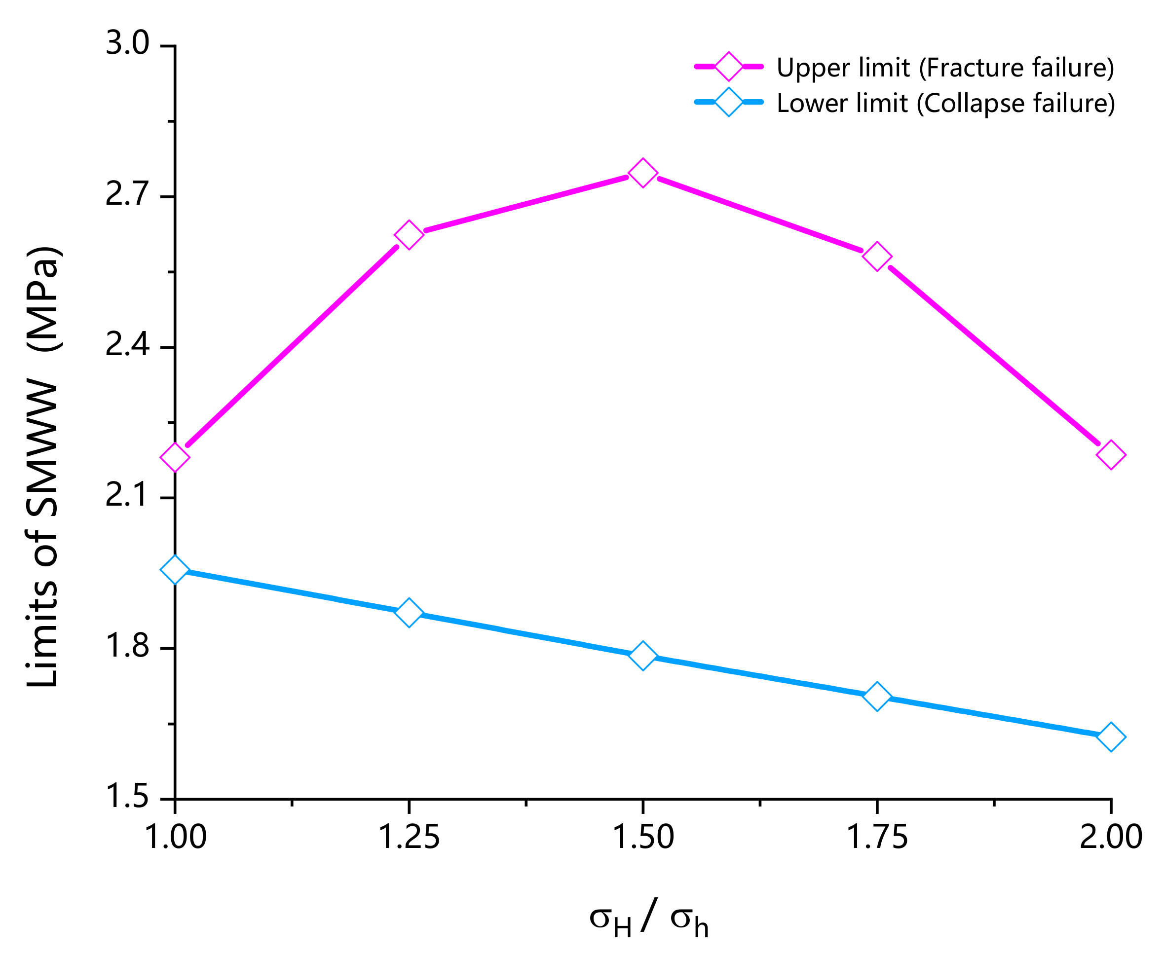
5.2.1. In Situ Stress

The influence of in situ stress on wellbore stability is studied under the normal-faulting (NF) in situ stress regime. Under the NF regime, there is ${\sigma }_v>{\sigma }_H>{\sigma }_h$. From Figure 6, it is convenient to obtain the upper and lower limit of the safe wellbore pressure window. In the following figures, the safe mud weight window (SMWW) is calculated and analyzed as this concept is much easier to be understood in drilling engineering. Under the assumption of static state, the SMWW is actually the ratio of safe wellbore pressure window and mud density. In Figure 7, the upper and lower limits of safe mud weight window are calculated and illustrated, respectively. It is seen under the NF regime, when the ratio of ${\sigma }_H/{\sigma }_h$ increases, the lower limit of SMWW gradually decreases while the upper limit first increases then decreases. In addition, the SMWW also first increases and then decreases. The change range of the SMWW is quite significant. This means the ratio of ${\sigma }_H/{\sigma }_h$ affects the failure of wellbore significantly and precise measurement of in situ stress underground is significant for the prediction of wellbore stability.

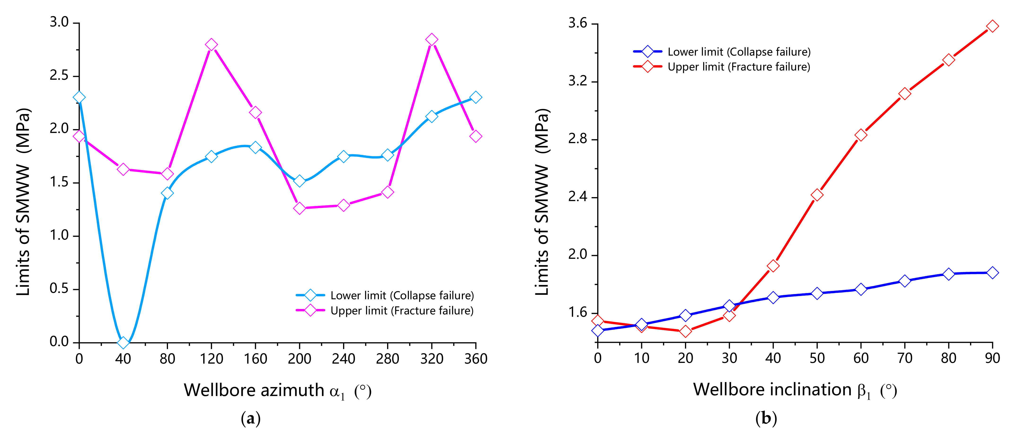
5.2.2. Orientation of Wellbore

To study how the SMWW change with different wellbore orientations, Figure 8 shows the results with the variation of wellbore azimuth (${\alpha }_1$) and inclination (${\beta }_1$), respectively. From Figure 8a, it is found both positive and negative SMWW exist while the wellbore azimuth change. For example, when ${\alpha }_1$ = 20~160°, a common positive SMWW exists; however, when ${\alpha }_1$ = 200~240°, a negative SMWW appears and under this condition, failures will inevitably happen. Therefore, to optimize the wellbore trajectory is quite necessary in drilling engineering as some directional borehole will always fail whatever the mud weight is. The same conclusion can be drawn by Figure 8b. As we can see, the SMWW will be narrow or negative when ${\beta }_1$ < 30° while the SMWW will be wider when the wellbore becomes more inclined. This means under this condition (Table 1), the more inclined (or horizontal) wells will be much safer than the less inclined (or vertical) wells.

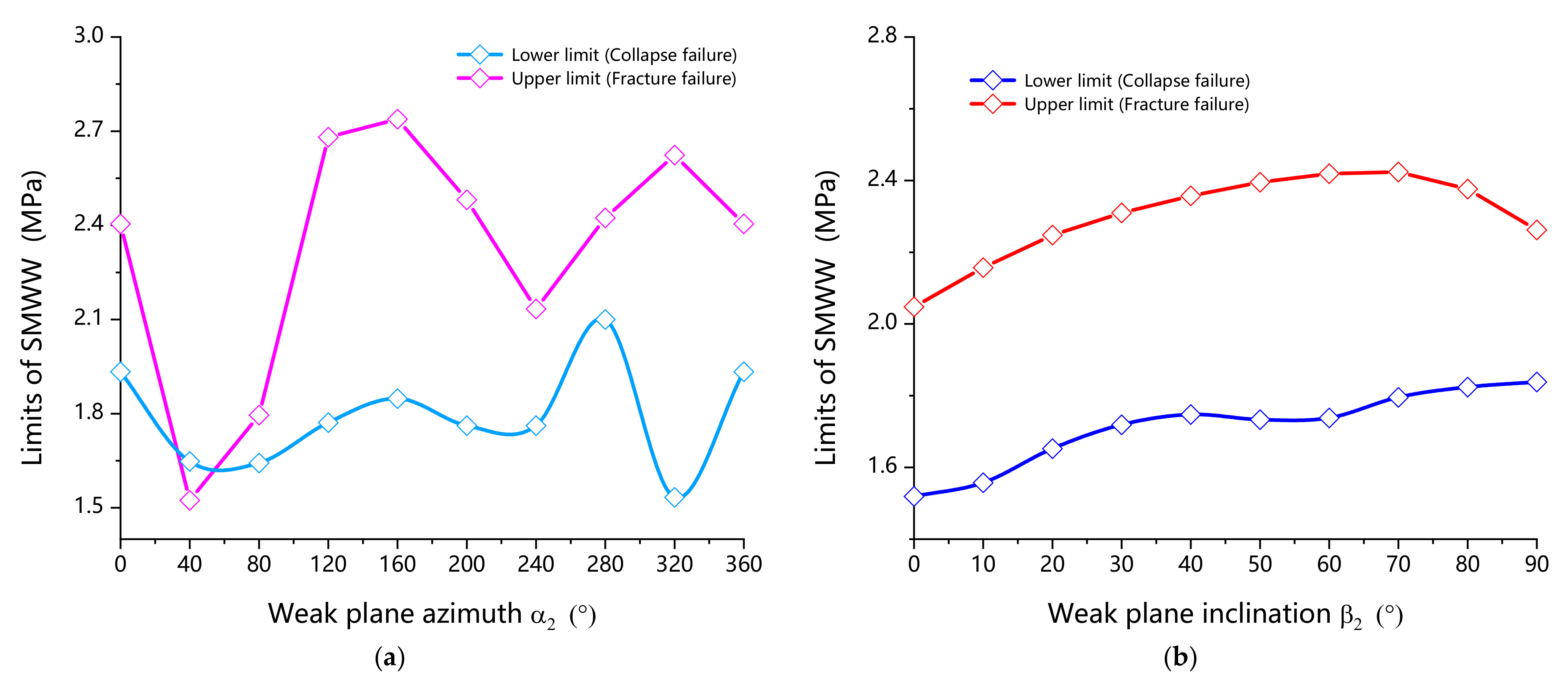
5.2.3. Orientation of Weak Planes

To investigate how the direction of formation influences the wellbore stability, Figure 9 shows the results of SMWW affected by the azimuth (${\alpha }_2$) and inclination (${\beta }_2$) of bedding planes. From Figure 9b, it is seen that the upper and lower limit of SMWW gradually change with the increase of bedding’s inclination. This means the change of SMWW will be moderate if only the weak planes become more inclined without changing the azimuth. However, in Figure 9a, it is found the SMWW will change greatly when the azimuth of weak planes changes. Therefore, one should pay more attention to the azimuth of weak planes while planning the mud weight for drilling.

5.2.4. Elastic Anisotropy

Rocks with bedding planes are intrinsically anisotropic with regard to both strength and elastic characteristics. As strength anisotropy only affects the failure criterion of rocks, the elastic anisotropy of rocks will be studied in this section. From Section 2.2, it is noted the elastic parameters can affect the stress distribution around the wellbore. Bedding rocks can be regarded as transversely isotropic; therefore, it is important to know how the vertical and horizontal (as to the bedding planes) elastic parameters affect the safety of wellbore.

In Figure 10a, the ratio of $E_h/E_v$ changes and the resulted SMWW are shown. It is found that both the upper and lower limit of SMWW decrease with the increase of $E_h/E_v$ but the upper limit decreases more rapidly than the lower limit, which resulted in a narrower SMWW with higher $E_h/E_v$. This means the change of $E_h/E_v$ will affect the upper limit of SMWW much greater than the lower limit, and a more anisotropic Young’s modulus will result in a narrower SMWW. From Figure 10b, it is seen with the increase of ${\upsilon }_v/{\upsilon }_h$, the upper limit of SMWW gradually increases while the lower limit of SMWW changes a little. This means a more anisotropic Poisson’s ratio will result in a wider SMWW. Comparing Figure 10a,b, the same conclusion can be made that the effects of elastic anisotropy are greater on the upper limit of SMWW than the lower limit. However, the differences are reflected in two aspects: one is that with the increase of different elastic anisotropy, the change trend of SMWW is different; the other is that the effects of Poisson’s ratio are slighter than Young’s modulus.

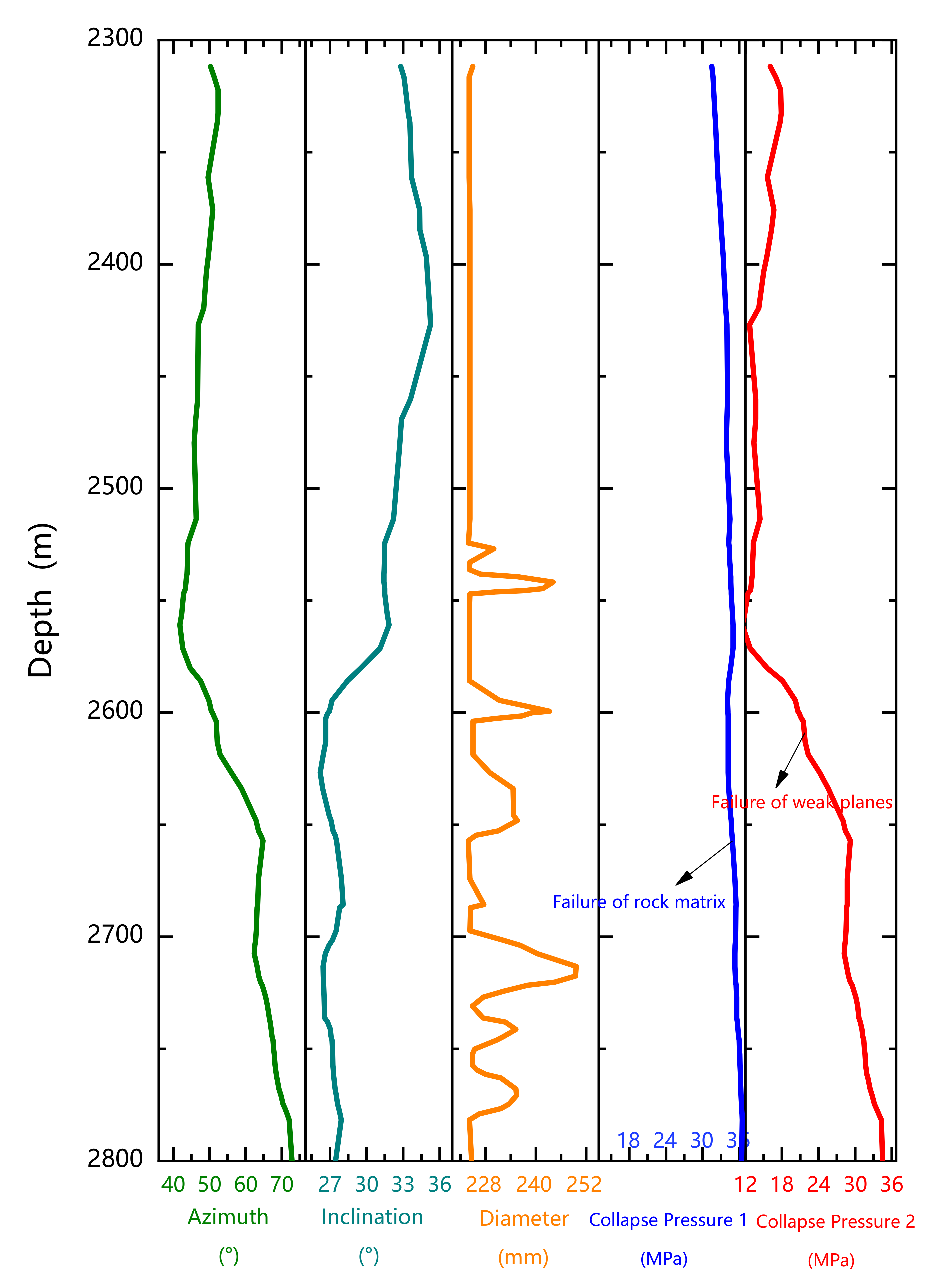
5.3. Real-Time Calculation and Prediction in Drilling Process

As the drilling process is ongoing, it is important to control the weight of drilling mud to maintain wellbore stability in real time. However, the factors related to drilling safety, such as environment and trajectory, may change with depth. In particular, the orientation of the wellbore may change constantly, as shown by Figure 11. Under this condition, having a precise prediction of the real-time mud weight becomes quite essential for guiding safe drilling. The mathematical model built in this paper and the programing scheme developed can thus be very helpful.

As shown in Figure 11, in the depth range of 2300~2800 m, both the azimuth and inclination of the wellbore change constantly due to limited control of drilling equipment. Especially when the depth > 2600 m, the azimuth and inclination have greater variations. In addition, the borehole diameter detected by downhole tools is also shown in this figure. By using the real-time prediction method illustrated by former parts, the collapse pressures at different depths are calculated and shown in Figure 11. It is noted that the real field data in the Boulder area [46] are applied in the following calculations. The elastic and strength properties of rocks are assumed to be constant with depth (Table 1) as shales constitute the main contents of the formation, especially below 2600 m where severe failures occur. According to the reference, no significant changes regarding the orientation of beddings and in situ stresses were detected in this area, therefore these parameters are assumed to be unchanged with depth and the in situ stresses are set to be ${\sigma }_H$ = 28 MPa/km, ${\sigma }_h$ = 20 MPa/km, and ${\sigma }_v$ = 25 MPa/km. From Figure 11, it is seen that both the collapse pressures considering the failure of rock matrix and weak planes are calculated. On the whole, it is clearly seen that the prediction results are in accordance with the in situ data. When the depth > 2600 m, the collapse pressure calculated enlarges greatly compared to the shallower depth. In the meantime, severe instability issues actually occur during this depth range as expanding diameter is frequently encountered. It is noted that a constant mud weight is actually used in the drilling process of the Boulder 3#, therefore a higher collapse pressure would mean failure of the wellbore (or expanding diameter) happens. In addition, if we compare the last two columns of Figure 11, it is found that the collapse pressure determined by failure of weak planes increases greater than that determined by rock matrix. This means the anisotropic effects cannot be neglected if precise assessment of wellbore stability is needed while drilling in bedding formations.

6. Conclusions

A novel wellbore stability model considering both elastic and strength anisotropy of bedding formations is presented in this paper. The method for real-time prediction of stress distribution, failure and safe mud weight in real time is developed. Based on the calculation results and analyses of the case in the real field, the following conclusions can be drawn:

• Based on the model built in this paper and the method developed for programming, it is convenient to calculate the stress distribution, failure area, collapse and fracture pressure around a general wellbore in anisotropic bedding formations.
• All the factors of in situ stress, directions of wellbore and weak planes, and anisotropic elastic parameters have significant influences on the SMWW: the ratio of horizontal in situ stress (${\sigma }_H/{\sigma }_h$) and elastic parameters ($E_h/E_v$, ${\upsilon }_v/{\upsilon }_h$) affect the upper limit of SMWW greater than the lower limit; negative SMWW may appear with the change of the wellbore’s (or weak plane’s) orientation, especially when the azimuth of the well (weak plane) changes; considering elastic anisotropy, the effects of Young’s modulus on the SMWW is greater than the Poisson’s ratio.
• The anisotropic characteristics of bedding rocks cannot be neglected when assessing wellbore stability and the method established in this paper can greatly help with the precise prediction of safety issues as drilling proceeds.

References

1. Steiger, R.P.; Leung, P.K. Quantitative Determination of the Mechanical Properties of Shales. SPE Drill. Eng. 1992, 7, 181–185. [Google Scholar] [CrossRef]
2. Gaede, O.; Karpfinger, F.; Jocker, J.; Prioul, R. Comparison between Analytical and 3D Finite Element Solutions for Borehole Stresses in Anisotropic Elastic. Int. J. Rock Mech. Min. Sci. 2012, 51, 53–63. [Google Scholar] [CrossRef] [Green Version]
3. Meier, T.; Rybacki, E.; Backers, T.; Dresen, G. Influence of Bedding Angle on Borehole Stability: A Laboratory Investigation of Transverse Isotropic Oil Shale. Rock Mech. Rock Eng. 2015, 48, 1535–1546. [Google Scholar] [CrossRef]
4. Lee, H.; Ong, S.H.; Azeemuddin, M.; Goodman, H. A Wellbore Stability Model for Formations with Anisotropic Rock Strengths. J. Pet. Sci. Eng. 2012, 96–97, 109–119. [Google Scholar] [CrossRef]
5. Nasseri, M.H.B.; Rao, K.S.; Ramamurthy, T. Anisotropic Strength and Deformational Behavior of Himalayan Schists. Int. J. Rock Mech. Min. Sci. 2003, 40, 3–23. [Google Scholar] [CrossRef]
6. Aadnoy, B.; Hareland, G.; Kustamsi, A.; de Freitas, T.; Hayes, J. Borehole Failure Related to Bedding Plane. In Proceedings of the 43rd US Rock Mechanics Symposium & 4th US-Canada Rock Mechanics Symposium 2009, Asheville, NC, USA, 28 June–1 July 2009. [Google Scholar]
7. Chenevert, M.E.; Gatlin, C. Mechanical Anisotropies of Laminated Sedimentary Rocks. Soc. Pet. Eng. J. 1965, 5, 67–77. [Google Scholar] [CrossRef]
8. Geng, Z.; Chen, M.; Jin, Y.; Yang, S.; Yi, Z.; Fang, X.; Du, X. Experimental Study of Brittleness Anisotropy of Shale in Triaxial Compression. J. Nat. Gas Sci. Eng. 2016, 36, 510–518. [Google Scholar] [CrossRef]
9. Yan, C.; Deng, J.; Cheng, Y.; Li, M.; Feng, Y.; Li, X. Mechanical Properties of Gas Shale During Drilling Operations. Rock Mech. Rock Eng. 2017, 50, 1753–1765. [Google Scholar] [CrossRef]
10. Gale, J.F.W.; Holder, J. Natural Fractures in the Barnett Shale: Constraints on Spatial Organization and Tensile Strength with Implications for Hydraulic Fracture Treatment in Shale-Gas Reservoirs. In Proceedings of the 42nd US Rock Mechanics Symposium (USRMS), San Francisco, CA, USA, 29 June–2 July 2008. [Google Scholar]
11. Mokhtari, M.; Tutuncu, A.N. Impact of Laminations and Natural Fractures on Rock Failure in Brazilian Experiments: A Case Study on Green River and Niobrara Formations. J. Nat. Gas Sci. Eng. 2016, 36, 79–86. [Google Scholar] [CrossRef]
12. Niandou, H.; Shao, J.F.; Henry, J.P.; Fourmaintraux, D. Laboratory Investigation of the Mechanical Behaviour of Tournemire Shale. Int. J. Rock Mech. Min. Sci. 1997, 34, 3–16. [Google Scholar] [CrossRef]
13. Wang, Z. Seismic Anisotropy in Sedimentary Rocks, Part 2: Laboratory Data. Geophysics 2002, 67, 1423–1440. [Google Scholar] [CrossRef]
14. Cho, J.-W.; Kim, H.; Jeon, S.; Min, K.-B. Deformation and Strength Anisotropy of Asan Gneiss, Boryeong Shale, and Yeoncheon Schist. Int. J. Rock Mech. Min. Sci. 2012, 50, 158–169. [Google Scholar] [CrossRef]
15. Ong, S.H. Borehole Stability. Ph.D. Thesis, The University of Oklahoma, Norman, OK, USA, 1994. [Google Scholar]
16. Suarez-Rivera, R.; Green, S.J.; McLennan, J.; Bai, M. Effect of Layered Heterogeneity on Fracture Initiation in Tight Gas Shales. In Proceedings of the SPE Annual Technical Conference and Exhibition 2006, San Antonio, TX, USA, 24–27 September 2006. [Google Scholar]
17. Bradley, W.B. Failure of Inclined Boreholes. J. Energy Resour. Technol. 1979, 101, 232–239. [Google Scholar] [CrossRef]
18. Ding, L.; Wang, Z.; Liu, B.; Lv, J. Assessing Borehole Stability in Bedding-Parallel Strata: Validity of Three Models. J. Pet. Sci. Eng. 2019, 173, 690–704. [Google Scholar] [CrossRef]
19. Wang, J.; Weijermars, R. New Interface for Assessing Wellbore Stability at Critical Mud Pressures and Various Failure Criteria: Including Stress Trajectories and Deviatoric Stress Distributions. Energies 2019, 12, 4019. [Google Scholar] [CrossRef] [Green Version]
20. Detournay, E.; Cheng, A.H.-D. Poroelastic Response of a Borehole in a Non-Hydrostatic Stress Field. Int. J. Rock Mech. Min. Sci. Geomech. Abstr. 1988, 25, 171–182. [Google Scholar] [CrossRef]
21. Cui, L.; Abousleiman, Y.; Cheng, A.H.-D.; Roegiers, J.-C. Time-Dependent Failure Analysis of Inclined Boreholes in Fluid-Saturated Formations. J. Energy Resour. Technol. 1999, 121, 31. [Google Scholar] [CrossRef]
22. Ding, L.; Wang, Z.; Liu, B.; Lv, J.; Wang, Y. Borehole Stability Analysis: A New Model Considering the Effects of Anisotropic Permeability in Bedding Formation Based on Poroelastic Theory. J. Nat. Gas Sci. Eng. 2019, 69, 102932. [Google Scholar] [CrossRef]
23. McTigue, D.F. Thermoelastic Response of Fluid-Saturated Porous Rock. J. Geophys. Res. 1986, 91, 9533. [Google Scholar] [CrossRef]
24. Kurashige, M. A Thermoelastic Theory of Fluid-Filled Porous Materials. Int. J. Solids Struct. 1989, 25, 1039–1052. [Google Scholar] [CrossRef]
25. Wu, B.; Zhang, X.; Jeffrey, R.G.; Wu, B. A Semi-Analytic Solution of a Wellbore in a Non-Isothermal Low-Permeability Porous Medium under Non-Hydrostatic Stresses. Int. J. Solids Struct. 2012, 49, 1472–1484. [Google Scholar] [CrossRef] [Green Version]
26. Ding, L.; Wang, Z.; Wang, Y.; Liu, B. Thermo-Poro-Elastic Analysis: The Effects of Anisotropic Thermal and Hydraulic Conductivity on Borehole Stability in Bedding Formations. J. Pet. Sci. Eng. 2020, 190, 107051. [Google Scholar] [CrossRef]
27. Huan, X.; Xu, G.; Zhang, Y.; Sun, F.; Xue, S. Study on Thermo-Hydro-Mechanical Coupling and the Stability of a Geothermal Wellbore Structure. Energies 2021, 14, 649. [Google Scholar] [CrossRef]
28. Chen, X.; Tan, C.P.; Detournay, C. A Study on Wellbore Stability in Fractured Rock Masses with Impact of Mud Infiltration. J. Pet. Sci. Eng. 2003, 38, 145–154. [Google Scholar] [CrossRef]
29. Kanfar, M.F.; Chen, Z.; Rahman, S.S. Analyzing Wellbore Stability in Chemically-Active Anisotropic Formations under Thermal, Hydraulic, Mechanical and Chemical Loadings. J. Nat. Gas Sci. Eng. 2017, 41, 93–111. [Google Scholar] [CrossRef]
30. Aslannezhad, M.; Keshavarz, A.; Kalantariasl, A. Evaluation of Mechanical, Chemical, and Thermal Effects on Wellbore Stability Using Different Rock Failure Criteria. J. Nat. Gas Sci. Eng. 2020, 78, 103276. [Google Scholar] [CrossRef]
31. Li, X.; Jaffal, H.; Feng, Y.; El Mohtar, C.; Gray, K.E. Wellbore Breakouts: Mohr-Coulomb Plastic Rock Deformation, Fluid Seepage, and Time-Dependent Mudcake Buildup. J. Nat. Gas Sci. Eng. 2018, 52, 515–528. [Google Scholar] [CrossRef]
32. Guo, Z.Y.; Wang, H.N.; Jiang, M.J. Elastoplastic Analytical Investigation of Wellbore Stability for Drilling in Methane Hydrate-Bearing Sediments. J. Nat. Gas Sci. Eng. 2020, 79, 103344. [Google Scholar] [CrossRef]
33. He, S.; Wang, W.; Zhou, J.; Huang, Z.; Tang, M. A Model for Analysis of Wellbore Stability Considering the Effects of Weak Bedding Planes. J. Nat. Gas Sci. Eng. 2015, 27, 1050–1062. [Google Scholar] [CrossRef]
34. Ma, T.; Zhang, Q.B.; Chen, P.; Yang, C.; Zhao, J. Fracture Pressure Model for Inclined Wells in Layered Formations with Anisotropic Rock Strengths. J. Pet. Sci. Eng. 2017, 149, 393–408. [Google Scholar] [CrossRef]
35. Deangeli, C.; Omwanghe, O. Prediction of Mud Pressures for the Stability of Wellbores Drilled in Transversely Isotropic Rocks. Energies 2018, 11, 1944. [Google Scholar] [CrossRef] [Green Version]
36. Lekhnitskii, S.G.; Fern, P.; Brandstatter, J.J.; Dill, E.H. Theory of Elasticity of an Anisotropic Elastic Body. Phys. Today 1964, 17, 84. [Google Scholar] [CrossRef]
37. Amadei, B. Rock Anisotropy and the Theory of Stress Measurements; Lecture Notes in Engineering; Springer: Berlin/Heidelberg, Germany, 1983; Volume 2, ISBN 978-3-540-12388-0. [Google Scholar]
38. Aadnoy, B.S. Modelling of the Stability of Highly Inclined Boreholes in Anisotropic Rock Formations. SPE Drill. Eng. 1987, 3, 259–268. [Google Scholar] [CrossRef]
39. Aadnoy, B.S.; Ong, S. Introduction to Special Issue on Borehole Stability. Boreh. Stab. 2003, 38, 79–82. [Google Scholar] [CrossRef]
40. Ding, L.; Wang, Z.; Lv, J.; Wang, Y.; Liu, B. New Methodology to Determine the Upper Limit of Safe Borehole Pressure Window: Considering Compressive Failure of Rocks While Drilling in Anisotropic Shale Formations. J. Nat. Gas Sci. Eng. 2021, 96, 104299. [Google Scholar] [CrossRef]
41. Setiawan, N.B.; Zimmerman, R.W. Wellbore Breakout Prediction in Transversely Isotropic Rocks Using True-Triaxial Failure Criteria. Int. J. Rock Mech. Min. Sci. 2018, 112, 313–322. [Google Scholar] [CrossRef]
42. Al-Ajmi, A.M.; Zimmerman, R.W. Stability Analysis of Vertical Boreholes Using the Mogi–Coulomb Failure Criterion. Int. J. Rock Mech. Min. Sci. 2006, 43, 1200–1211. [Google Scholar] [CrossRef]
43. Zhang, L.; Cao, P.; Radha, K.C. Evaluation of Rock Strength Criteria for Wellbore Stability Analysis. Int. J. Rock Mech. Min. Sci. 2010, 47, 1304–1316. [Google Scholar] [CrossRef]
44. Gholami, R.; Moradzadeh, A.; Rasouli, V.; Hanachi, J. Practical Application of Failure Criteria in Determining Safe Mud Weight Windows in Drilling Operations. J. Rock Mech. Geotech. Eng. 2014, 6, 13–25. [Google Scholar] [CrossRef] [Green Version]
45. Jaeger, J.C.; Cook, N.G.W.; Zimmerman, R.W. Fundamentals of Rock Mechanics, 4th ed.; Blackwell Pub: Malden, MA, USA, 2007; ISBN 978-0-632-05759-7. [Google Scholar]
46. McLellan, P.J.; Cormier, K. Borehole Instability in Fissile, Dipping Shales, Northeastern British Columbia. In Proceedings of the SPE Gas Technology Symposium 1996, Calgary, AB, Canada, 28 April–1 May 1996. [Google Scholar]
Figure 1. Deviated wellbore drilling in bedding formation with weak planes.
Energies 15 00251 g001
Figure 2. General relations between different coordinate systems in underground space: (a) relation between GCS (Xg, Yg, Zg) and WCS (Xb, Yb, Zb); (b) relation between GCS and WPCS (Xw, Yw, Zw).
Energies 15 00251 g002
Figure 3. Method flowchart for the real-time safe mud weight prediction using software programing.
Energies 15 00251 g003
Figure 4. Stress distribution in the: (a) hoop direction around the wellbore; (b) radial direction of θ = 30° around the wellbore. The criteria index of Mogi–C and M–C are also illustrated.
Energies 15 00251 g004
Figure 5. Failure area around the wellbore (Table 1) based on the failure criterion of: (a) rock matrix; (b) weak planes.
Energies 15 00251 g005
Figure 6. Collapse pressure, fracture pressure and the related safe wellbore pressure window for the wellbore in Boulder area (Table 1).
Energies 15 00251 g006
Figure 7. The effects of the ratio of σ H / σ h on the limits of safe mud weight window (SMWW). The normal-faulting (NF) regime is under consideration.
Energies 15 00251 g007
Figure 8. Variation of SMWW with the change of: (a) wellbore azimuth α 1 ; (b) wellbore inclination β 1 .
Energies 15 00251 g008
Figure 9. Variation of SMWW with the change of: (a) weak-plane azimuth α 2 (b) weak-plane inclination β 2 .
Energies 15 00251 g009
Figure 10. The change of SMWW that affected by the ratio of: (a) E h / E v ; (b) υ v / υ h .
Energies 15 00251 g010
Figure 11. The variation of in situ field data (including the azimuth, inclination and diameter of wellbore) with depth in Boulder 3# and the prediction results of collapse pressure according to the new method.
Energies 15 00251 g011