Abstract
The Scheffler type concentrator is a curved metal reflector particularly suitable for solar thermal systems with a receiver fixed to the ground. Its operating principle is to deform the reflector throughout the year to optimize its performance in collecting sunlight. This study analyses the optical performance of a Scheffler reflector during the year. A CAD software tool is utilized to reproduce the mechanical deformations of a real Scheffler concentrator and the shape of the light spot on the receiver is analyzed by means of raytracing simulations. The starting configuration is the equinoctial paraboloid, which produces a point-like spot on the two equinox days only. On all other days of the year, this paraboloid is deformed in a suitable way in order to keep the spot as small as possible, but, even so, it is no longer a point-like spot. In the present work the simulated light distributions on the receiver, generated by the paraboloids (deformed or original), are compared. The results confirm the working principle of the Scheffler type concentrator and allow correctly sizing the receiver.
1. Introduction
Combating climate change needs to exploit, in the best possible way, solar radiation, a famously renewable energy source.
Currently, solar energy is mainly exploited for electricity production, especially by means of photovoltaic panels, but the production of thermal energy is also gaining interest and efforts are currently being made to reduce the installation costs of such production. All current systems to produce thermal energy consist of one or more mirrors (seldom lenses) that redirect solar radiation towards a small target, but there are various types of solar device, such as concentrating systems, point focus collectors, linear array; each one is designed to be applied to a specific thermal energy production method.
It should be considered that, in choosing the system to be implemented, some factors are often preponderant, such as efficiency, complexity, costs of implementation and maintenance.
Solar systems that use thermal receivers must necessarily use pipes to transport the heat-transfer fluid. For this reason, it is advantageous to fix the receiver to the ground and move only the concentrator mirror.
From the literature it is clear that the Scheffler-type configuration is a suitable configuration for this purpose, especially considering its low production cost and its simplicity of manufacturing, which is shown in [1], where is presented a comparison of some fixed-focus parabolic systems, relying on the parameters that affect their efficiency.
Several articles describe how to design and build Scheffler mirrors, from either a geometric-mechanical [2,3,4] or a mathematical [5] point of view.
In the literature there are various examples of applications, especially for desalination purposes, solar cooking, agriculture [6], and for the production of electricity [7,8].
The Scheffler configuration utilizes an equatorial mount with a parabolic concentrator, which must be mechanically deformed, daily, during the year to keep an acceptable concentration level of solar radiation. Often these deformations have manual regulation. The reason for this deformation is well explained in the article by Panchal et al. [7], “The mirror has to be occasionally titled about a perpendicular axis to compensate for the seasonal variation in the sun’s declination.” … “A framework that supports the reflector includes a mechanism that can be used to tilt it and also bend it appropriately. The mirror is never exactly paraboloid, but it is always close enough towards the receiver” [7]. Ruelas et al. in [1] report that “It also features a daily tracking mechanism based on an adjustable bar and a central pivot that changes the reflector inclination to produce a maximum aperture variation of ±8%”. Rapp et al. in [4] realize an alternative configuration in which the receiver is not on the floor, but is in a higher position with respect to the mirror, which is placed almost horizontally. Reddy et al. in [5] explain that “Two telescopic clamps with locks are provided at the top and bottom of the reflector…”. In order to refocus solar radiation back at F, the two telescopic clamps are unlocked and the parabola is manually tilted towards the sun’s new position” [5]. Islam et al. in [8] declare that “The paraboloid shape is obtained by rearranging the mirrors in order to reflect the incident solar rays to a common focus of the collector”. Vyas et al. in [9] state that “The dish uses automatic daily tracking and manual seasonal tracking mechanism to ensure maximum optical efficiency of the Scheffler dish solar collector”.
In order to allow easy manufacturing, this concentrator is often composed of several elementary mirrors. Concerning the mosaic mirror, Reddy et al. in [5] affirm that “Mirror size plays an important role in proper functioning of reflector surface. Smaller the mirror size better will be the concentration due to better fitting into the reflector profile curvature…”. A code in MATLAB is developed, which requires square mirror size as an input for a Scheffler reflector of given focal length and aperture area. The output of the code is the total number of mirrors required and their arrangement over the reflector profile” [5].
Mechanical deformation is needed to limit the variation of the spot size on the receiver; indeed, the parabola, the shape of which has been theoretically calculated for a determined day of the year (very often the equinox), has to be adapted for the other days. So, a large increase of the spot size is avoided, as it would inevitably lead to a lower concentration ratio, which instead should be high, especially in the applications where high temperature values are an issue. In fact, attempts have been published to control the concentration of the system [9].
The size of the image also affects the size of both the receiver and the eventual secondary optics. Malwad et al. in [10] analyze three receiver versions: “In these experiments, a receiver with three different types of arrangement was tested under identical solar radiation condition…”. In this experiment, under average beam radiation 640 W/m2 receiver temperature of 241 °C, 266 °C, 253 °C was achieved with first, second and third arrangement. The average thermal efficiency of the receiver for first, second and third arrangements has been calculated 57.71%, 60.93% and 68.03%, receiver cover with tube coil increases the overall efficiency of the system” [10]. In this study, the receiver with the third arrangement was found efficient, while, in [11], Ruelas et al. found that the more suitable geometry for the receiver has an elliptical form. Kumar et al. in [12] analyze six different shapes of receiver, though each with equal aperture and depth. The study was conducted to examine convective heat losses. The results show that “among the six shapes analyzed, the cone-cylindrical cavity is the most efficient in terms of solar flux utilization whereas hemispherical cavity results in maximum heat loss” [12].
The aim of our work is to evaluate, by means of raytracing techniques, the spot on the receiver as a function of the shape of the Scheffler concentrator, deformed to optimize its performance in sunlight collection.
This analysis of a Scheffler receiver, with purely optical methodologies, represents a novelty. Design methods can be found in the literature that are based only on mechanical studies, but none of these employ raytracing methods developed for the design of optical systems. The joint use of CAD3D software and commercial raytracing software makes it possible to predict the shape and irradiance map of the light spot on the receiver. This optical raytracing analysis is easily applicable to evaluating the use of a Scheffler-type concentrator for a specific application.
The initial study is dedicated to a system with a continuous mirror because it is simpler to design and serves to help in understanding the feasibility and performance of the system under examination.
The transition to a mosaic mirror is strongly influenced by the sizing of the input opening of the receiver; in fact, the minimum size of the spot is determined by the dimensions of the elementary mirror. However, in this case, the surface where the mosaic of mirrors will be allocated is a continuous one.
The proposed analysis method allows predicting the shape of the light spot on the receiver as a function of the deformations applied to the mirror.
The starting configuration is the paraboloid designed for the equinox, which produces, on the receiver, a spot that is perfectly focused on that day only.
This article is divided into sections, which illustrate the development of the raytracing simulations that are combined to reproduce these mechanical deformations. These studies employ two software packages: Zemax-OpticStudio, for raytracing analyses, and SolidWorks, to reproduce the mechanical deformations of the actual paraboloid.
2. Optical Design of a Scheffler Concentrator
The Scheffler-type concentrator (Figure 1 and Figure 2) is the most cited in the literature for applications with a receiver fixed to the ground. In theory there could be a paraboloid for only each day of the year, with the axis directed at all times towards the sun and the focus at the same point; the problem, here, is that this paraboloid should not only be rotated but also translated to have the focus always in the same point, and the translation operation is difficult, especially for objects of considerable size.
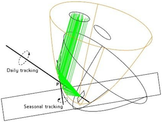
Figure 1.
Parabolas calculated for the equinox (black) and for the summer solstice (orange). The light beam has the direction it would have locally on 21 June. The figure shows the seasonal and daily axes that pass through the point P common to the two parabolas.
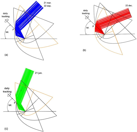
Figure 2.
Side view of the beam concentrated by the parabolas calculated for: Equinox (a), winter solstice (b), summer solstice (c), all passing through the same point P. Note that the distance PF remains the same.
To avoid the translation of the paraboloid, one might consider using paraboloids of different shapes that have a point on the surface and the focus in common. Some examples are shown in Figure 2.
Since this option is not feasible, only one paraboloid is used, optimized for the equinox but capable of deforming to approximate the paraboloids of different shapes that should be used. The paraboloid, therefore, does not translate but merely rotates.
The construction principle of a Scheffler-type concentrator is illustrated in Figure 1 and Figure 2. The different parabolas, which alternate throughout the year, lie around the point P and the seasonal axis.
In all raytracing simulations the sun is considered to be at noon.
The drawings in Figure 2 show three parabolas whose shapes are calculated, respectively, for the equinox (Figure 2a), the winter solstice (Figure 2b) and the summer solstice (Figure 2c). The parabolas have a common point P; the rotation happens both around the axis that connects the focus with the point P (daily rotation) and around the axis perpendicular to the previous one and parallel to the ground (seasonal rotation). In reality, the reflector is, physically, always the same, but its shape has to be continuously changed throughout the year by deformation.
Calculation of the Reflector Profile for a Certain Day of the Year
Figure 3 clarifies how to calculate the reflector shape. If a section of the paraboloid (on a plane that contains the axis) is considered, the equinoctial parabola passing through the point P(xP; yP) and which has focus on F(xF; yF) is represented in red color in the figure.
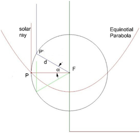
Figure 3.
Scheme of the construction of the reflector (in red). The equinoctial parabola crossing P focuses on F.
The generic equation of a parabola with vertical axis has the following expression:
y = a x2 + c
The focus of this parabola has coordinates:
yF = (4 a c + 1)/4 a
xF = 0
Therefore
and by imposing the passage for P:
4 a yF = 4 a c + 1
yP = a xP2 + c
c = yP − a xP2
Substituting Equation (6) into Equation (4)
4 a2 xP2 + 4 a (yF − yP) − 1 = 0
The values of a are obtained by solving Equation (6). If a point at the same height of F is chosen, with con yF = yP, the equation is further simplified. Once “a” is found, “c” is computed from Equation (6).
All the other parabolas relative to the other days of the year must have a point lying on the circle of radius d, which is the distance between F and P, as this is the location of the parabolas that have the same focal distance from F. Starting from the value of d, the parameters of the parabola of equation
are calculated for a certain day of the year by imposing that it passes through the point P(xP; yP) and that it has its focus on the focus of the equinoctial parabola.
y = a′ x2 + c′
In fact, knowing the declination α for that day, the coordinates of the point P′(x′P; y′P) are:
the parameters “a′” and “c′” are calculated by solving the equation of a parabola that passes through the point P(xP; yP) and with focus on F(0; yF).
x′P = xF + d cos(α)
y′P = yF + d sen(α)
Table 1 and Table 2 show the values of “a, “c” and the radius of curvature Rc for two values of the distance “d”: 2.7 m and 5 m. The value d = 2.7 m was obtained from an article by A. Munir et al. [2]. The value d = 5 m comes from considerations originating from a request to be able to concentrate a power of around 10,000 watts on the receiver.

Table 1.
Parameters defining the parabola and radius of curvature for d = 2.7 m.
Table 2.
Parameters defining the parabola and radius of curvature for d = 5 m.
The parabolas defined by the parameters of Table 1 and Table 2 have to be rotated by an angle β around the common focus F(xF; yF). The rotated parabolas are now able to concentrate the light rays coming from the ±β directions into focus F because the optical axis of the parabola has also been rotated by the same angle. Figure 4 presents the parabola profiles before and after rotation for the equinox, summer, and winter solstices.
The rotation formulas valid for each point of the parabola are:
x′ = (x − xF) cos(β) + (y − yF) sen(β) + xF
y′ = − (x − xF) sen(β) + (y − yF) cos(β) + yF
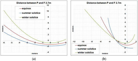
Figure 4.
Profiles of the parabolas calculated for the equinox and the two solstices, (a) before rotation and (b) after turning an angle β of ±23.5 degrees.
In the considered layout, the point P, which is common to all the parabolas, has the same y coordinate as the focus.
If the equinoctial parabola were utilized on the other days of the year, some image degradation would appear as an enlargement of the light spot on the receiver, as can be seen from the comparison between Figure 5 and Figure 6.
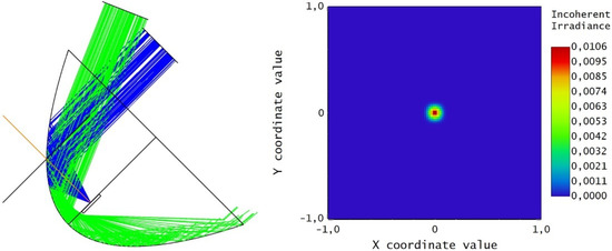
Figure 5.
Irradiance map on the receiver with the equinoctial parabola, calculated with the position of the sun at the equinox (blue rays). The green rays represent the position of the sun at the solstice. The irradiance values on the map are represented with an arbitrary scale.
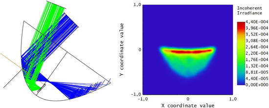
Figure 6.
Irradiance map on the receiver with the equinoctial parabola, calculated with the position of the sun at the solstice. The parabola has been rotated around the point indicated by the drawn cross until the receiver has been centered again. The position of the receiver is the same as that shown in Figure 5. The irradiance values on the map are represented with an arbitrary scale.
Figure 5 refers to the equinoctial parabola with the sun at the equinox, while Figure 6 shows the widening of the light spot on the receiver when the equinoctial parabola is used on the summer solstice. In this case, the simulation was obtained by rotating the equinoctial parabola at the point indicated by the cross until the receiver was centered again.
The sun is always considered to be at noon in the optical simulations.
The following optical simulation with the raytracing program (Zemax Optic Studio) requires knowledge of the radii of curvature Rc indicated in Table 1, as well as the distance d between the focus F and the center of rotation P.
In any case, it is mandatory to use a single reflector, because, due to its size and cost, it cannot be replaced many times during the year. Consequently, the profile of the reference parabola (the equinoctial one) must be continuously modified during the year [2,3].
The drawback to this is that the final mirror profile is not easily controllable, because the usual technique to adapt its shape is the deformation of the paraboloid by mechanical methods.
As previously discussed, after choosing the value of d, which represents the distance of the point P from the focus F on the receiver, the parameters “a”, “c” and the radius of curvature Rc of the paraboloid are calculated for certain days of the year. These Rc values will be used to simulate the optical system and the irradiance map on the receiver with a raytracing program (Zemax-OpticStudio). In Munir et al. [2,3], instead, it is defined a priori that the paraboloid has an elliptical shape with a known area. Three support points (pivot points) are then defined on this paraboloid, and they are used to rotate the structure and to deform it with the help of two linear actuators. On the basis of this information, the coefficients “a” and “c” are calculated; they are necessary to define the curvature of the paraboloid and to simulate the behavior of the light rays with Zemax-OpticStudio.
3. Mechanical and Optical Simulation
In order to study the optical behavior of a simulated Scheffler concentrator in the different operating conditions it was decided to deform the equinoctial paraboloid with the Solidworks 3D CAD software.
For this purpose, the “Flex-bending” feature was used to reproduce the deformations obtained by the lengthening or shortening of the two pistons. With this feature it is possible to flex a body by defining a bend axis; one that remains fixed and around which the body is bent, for which are also defined two trim planes that control what region of the body is flexed. Therefore, the deformation is achieved by setting a desired angle (or radius of curvature) between the two trim planes.
Table 3 shows the values of the coefficients of the three paraboloids as described in the Munir article [2]. The manufacturing data for the three paraboloids are:
collector area 8 m2
collector diameter 3.2 m
The values a and c in Table 3 refer to Equation (1).
Table 3.
Values of the coefficients of the three paraboloids in the Munir article [2].
Table 3.
Values of the coefficients of the three paraboloids in the Munir article [2].
| Summer Solstice (21 June) | Equinox (21 March; 22 September) | Winter Solstice (21 December) | |
|---|---|---|---|
| a | 0.28123 | 0.17447 | 0.12736 |
| c | 0.54394 | 0 | 0.53004 |
It is useful to specify, here, that the term parabola means the two-dimensional curve based on the parameters of Table 3 and Equation (8). Paraboloid, on the other hand, indicates the rotation surface obtained from the parabolic profile and intersected with a cylinder of suitable size. Therefore, the paraboloid is a three-dimensional object.
The actual manufactured mirror has the profile of the equinoctial equation (the equinoctial paraboloid indicated as “Par_0”). The mirror is mounted on a structure shown in Figure 7, which corresponds to Figure 9 at page 1499 of the article A. Munir et al./Solar Energy 84 (2010) 1490–1502 [2].
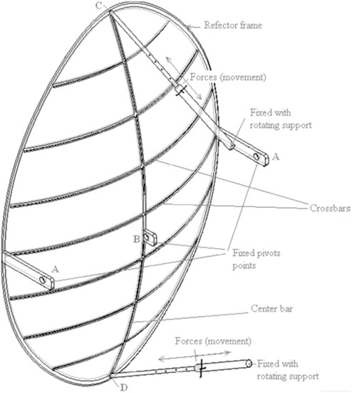
Figure 7.
Scheffler concentrator shown in Figure 9 of the article A. Munir et al./Solar Energy 2010, 84, 1490–1502 [2].
In this structure there are three fixed points, indicated as Pivots A (two points) and B, around which all the deformations take place. Figure 7 presents the Scheffler concentrator of the article by A. Munir [2].
The procedure can be outlined with the following steps:
Step 0—Original mirror: equinoctial paraboloid, indicated as “Par_0”.
Step 1—Rotation around Pivot B of the equinoctial paraboloid so that the local tangent of the rotation point is the same as the parabola of the analyzed day. The rotated paraboloid is indicated as “Par_1”.
Step 2—The action of the pistons in points C and D of the figure is reproduced by flexing the paraboloid around Pivot B. Since the real system has three fixed points, while the Solidworks function allows flexing only around one point, it was necessary to apply two deformations for every paraboloid to correctly simulate the effective action of the pistons on the mirror.
All the following figures presented in this section are based on the outputs of the CAD software SolidWorks.
In the Solidworks simulations, shown below, the bend axis matches to point B in such a way as to keep it stationary in two different directions: for the first deformation, the bend axis is perpendicular to the plane X–Y (passing through B) and the trim planes correspond to points C and D.
To complete the action of the pistons the equinoctial paraboloid was considered and the distance between the paraboloid edge and Pivots A was measured (23.5 cm), as was the distance established by the bars, visible in Figure 7. This distance is used for the second deformation, in order to match the edges of the bars with the border of the shifted paraboloid, due to the first deformation. In this second deformation, the bend axis is coincident with the tangent line of the parabola passing through B and results perpendicular to the first bend axis, while two trim planes correspond to points S and S′.
The paraboloid after the second bending is indicated as “Par_2”.
In the raytracing simulations the sun is always considered to be at noon.
The changes made on the equinoctial paraboloid (Par_0) to adapt it for the summer solstice are shown as an example.
The profiles (on the X–Y plane) of the ideal summer solstice parabola (in red, in Figure 8) and the rotated equinoctial parabola (in yellow, in Figure 8) were traced, both calculated from the values of Table 3.
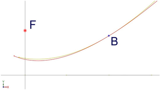
Figure 8.
Comparison between the correct summer solstice parabola (in red) and the rotated equinoctial parabola (in yellow).
The angle of rotation of the equinoctial parabola, in order to follow, as accurately as possible, the profile of the ideal summer solstice parabola, is 11.75 deg around Pivot B. The two parabolas are shown in Figure 8, while the two paraboloids are shown in Figure 9.
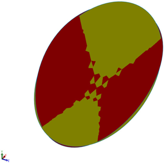
Figure 9.
Comparison between the paraboloid of the ideal summer solstice (in red) (Par_0s) and the rotated equinoctial paraboloid (in yellow) (Par_1s).
To compare the two paraboloids, a reference solstice paraboloid with an area equal to that of the equinoctial paraboloid was used, maintaining the same longitudinal diameter.
To simulate the actual deformation, we act directly on the paraboloid to modify its entire surface and not just on the profile of the generating parabola, starting with the first deformation. In Figure 10 are evidenced points C and D of the trim planes.
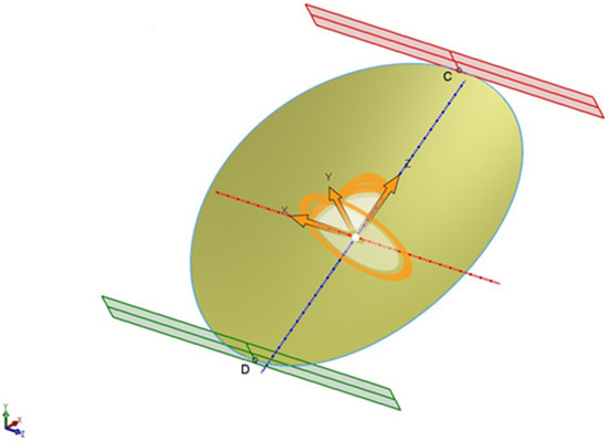
Figure 10.
Diagram of the first bending. Point B is stationary and the action has been taken on points C and D.
In this way it was possible to improve the overlap of the rotated equinoctial paraboloid profile with that of the paraboloid calculated for the summer solstice (ideal), the bending obtained is 5 degrees wide with a radius of curvature of 36.52 m. The results are shown in Figure 11. The yellow paraboloid, now, in some areas is more adherent to the reference paraboloid for the solstice (in red). However, the sides of the paraboloid are far from ideal.
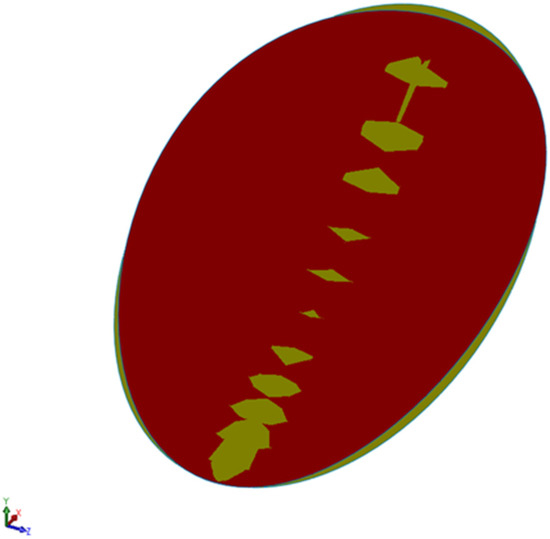
Figure 11.
Comparison between the paraboloid of the ideal summer solstice (Par_0s, in red) and the equinoctial paraboloid rotated and flexed by holding B fixed and acting on its points C and D (Par_2s, in yellow).
As explained before, for a correct simulation of the problem the two Pivots A must also remain in position. Figure 12 shows points S, S′, A and B. Since the two points are anchored to the edge of the paraboloid with two bars, the measured distance between Pivot A and edge of the paraboloid must remain constant. In particular, the constraints considered for the second deformation are the position on the X–Y plane of Pivots A and the length of the bars. The result of this movement is shown in Figure 13.
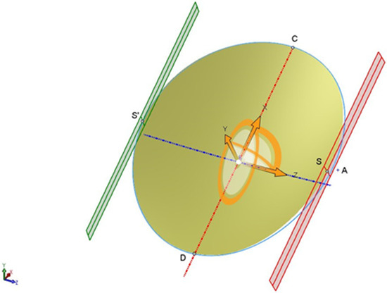
Figure 12.
Parabolas calculated for the equinox (black) and for the summer solstice (orange). The light beam has the direction it would have locally on 21 June. The figure shows the seasonal and daily axes that pass through the point P common to the two parabolas.
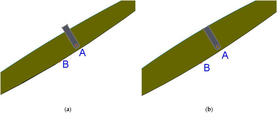
Figure 13.
Lateral view of the paraboloid, before the second bending (a) and after (b). Note that the edge of the paraboloid is in the correct position, at the end of the bar (b).
Now, the paraboloid has assumed the shape most similar to the real one; it is useful to note that the two paraboloids are now better overlapped, and the edges are very close together (Figure 14). The bending obtained with the second deformation is equal to −9 degrees with a radius of curvature of −18.91 m.
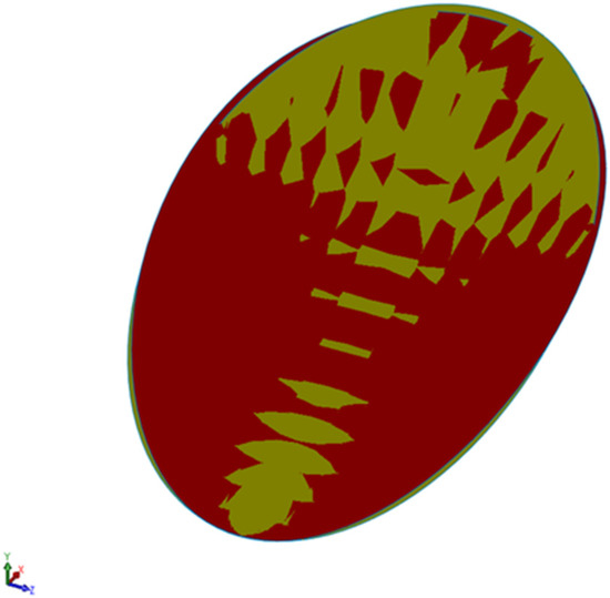
Figure 14.
Comparison between the paraboloid of the ideal summer solstice (Par_0s, in red) and the equinoctial paraboloid rotated and flexed twice (Par_2s, in yellow).
Table 4, Table 5 and Table 6 summarize the manufacturing data for each paraboloid. The tables also report the coordinates of the extreme points C and D and the areas of the paraboloids designed from the parameters of Table 3. The sign of the rotation angle is positive for counterclockwise rotations and negative for clockwise rotations. The positions of points C and D of Par_2s and Par_2w are particularly useful for obtaining the deformation that reaches the optimal configuration, from an optical point of view, as explained in Section 4.2.
Table 4.
Data of the paraboloids used for the simulations for the equinox.
Table 5.
Data of the paraboloids used for the simulations for the summer solstice.
Table 6.
Data of the paraboloids used for the simulations for the winter solstice.
Precise control and quantification of the mechanical deformations of the Scheffler reflector are essential for the correct operation of the Scheffler reflector to adapt it to every season. However, the innovative part consists in the raytracing study, which allows understanding the effects of these deformations on the image on the receiver.
4. Irradiance Maps on the Receiver
In order to evaluate the optical performance of the Scheffler concentrator, various simulations were performed using the Zemax-OpticStudio software. In particular, these raytracing simulations provide the irradiance maps of the solar radiation focused on the receiver. In the following figures the incoherent irradiance is reported in Watt/cm2.
The first series of simulations check the spot produced by the paraboloid after only step 1, i.e., the rotation around Pivot B of the equinoctial paraboloid (Par_0).
The second series of simulations considers the paraboloid produced by the bending; it can be considered as the real deformed paraboloid.
The figures below show the irradiance figures on the receiver calculated for noon, so they all have symmetry along the axes.
Considering the actual movement of the paraboloid during the day, it rotates around the center (0,0) with a clockwise angle equal to −15 degrees for each hour.
In order to evaluate the functioning of the system, a large target (1 m × 1 m), was employed, on which the irradiation maps and the average size of the spot were calculated. The target was placed so that the map of paraboloid 1 at the equinox was centered as seen in Figure 15.
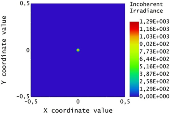
Figure 15.
Irradiance map for the equinoctial paraboloid at the equinox (Par_0).
4.1. Rotation around Pivot B
The collectors and the corresponding irradiance maps on the receiver are presented in Figure 16, Figure 17, Figure 18 and Figure 19. Figure 16 and Figure 18 show the paraboloids calculated by rotating the equinoctial paraboloid in the summer solstice and winter solstice positions, corresponding to the Par_1s and Par_1w of Table 5 and Table 6. Figure 17 and Figure 19 show the respective irradiance maps.
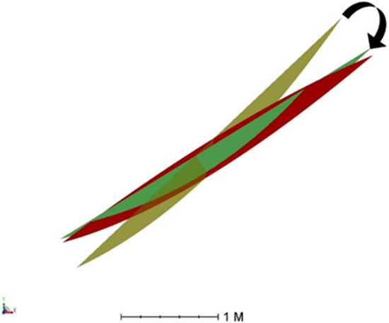
Figure 16.
Side view of the Par_0 (reference equinox, in yellow), Par_0s (summer solstice, in red) and Par_1s (Par_0 rotated as indicated by the arrow, in green).
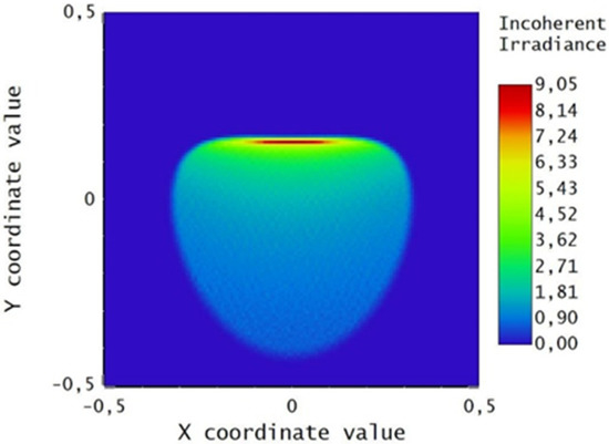
Figure 17.
Irradiance map for the equinoctial paraboloid rotated at the summer solstice Par_1s.
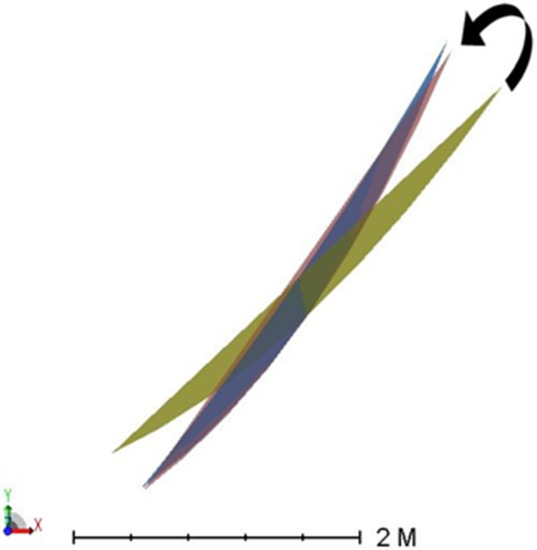
Figure 18.
Side view of the Par_0 (reference equinox, in yellow), Par_0w (winter solstice, in blue) and Par_1w (Par_0 rotated as indicated by the arrow, in pink).
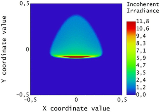
Figure 19.
Irradiance map for the equinoctial paraboloid rotated to the position of the winter solstice Par_1w.
4.2. Bending
Here, the paraboloids rotated in the previous step are bent. The bending decreases the beam size along the x direction. The collectors and the corresponding irradiance maps on the receiver are presented in Figure 20, Figure 21, Figure 22 and Figure 23. Figure 20 and Figure 22 report the side view of the real paraboloids Par_2s and Par_2w for the summer and winter solstices, respectively. The corresponding spots on the target are in Figure 21 and Figure 23.
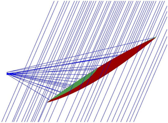
Figure 20.
Side view of Par_2s (green) superimposed to Par_0s (red), for the summer solstice.
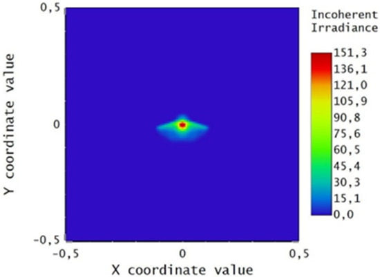
Figure 21.
Irradiance map for Par_2s.
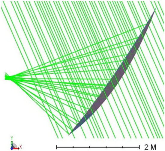
Figure 22.
Side view of Par_2w (pink) superimposed to Par_0w (blue), for the winter solstice.
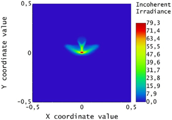
Figure 23.
Irradiance map for Par_2w.
The dimensions of the beam have decreased in both directions X and Y, although they are not as small as the focus in Figure 15.
The spot is smaller than that obtained with the previous procedure (Figure 17 and Figure 19). The more relevant difference is that the spots generated by parabolas Par_2w and Par_2s are not centered on the origin; this could be a problem in the case of a physical receiver, because the beam risks falling outside the receiver area.
Table 7, Table 8 and Table 9 show the data of the simulations carried out. For each configuration, whose data are shown in Table 4, Table 5 and Table 6, Table 7, Table 8 and Table 9 report the concentrated power (peak irradiance and total power) and the coordinates of the center of the spot on the target (the root–mean–square of the spot dimensions).
Table 7.
Numerical results of the simulations for the equinox.
Table 8.
Numerical results of the simulations for the summer solstice.
Table 9.
Numerical results of the simulations for the winter solstice.
For these simulations, the power of the source is set to 1 sun = 1000 W/m2 and the mirrors are considered ideal, so no losses are computed.
The paraboloid configurations, generated from the ideal parabolas, concentrate a spot on the target with highest peaks (elevated power) and smallest dimensions (focused image), as shown in Figure 16.
The tables show only the RMS of the spot size for the two final configurations for the summer and winter solstices, as they are the only ones corresponding to real situations and they are necessary to define the size of the receiver.
This study, with purely optical methodologies, to design a continuous mirror Scheffler system serves to help understand its feasibility for a specific application. The raytracing software furnishes the shape and irradiance map of the light spot on the receiver obtainable with different Scheffler-type reflectors. The various versions of the Scheffler reflector (experiencing mechanical deformations) have been compared. The illustrations in Section 3 evidence the differences from a mechanical the point of view. In Section 4, the light spot on the receiver is analyzed by an optical point of view. These optical analyses can be used to estimate the applicability of a Scheffler-type system for a particular configuration or in a defined system.
5. Sizing the Receiver
All previous efforts have been intended to set the size of the thermal system receiver. Considering that the spot has an asymmetrical shape, the size of the receiver must be as large as the major axis of the focused beam.
The previous analyses demonstrate that the worst case is the winter solstice: in this case the receiver, in order to collect more than 99% of the energy, must have a radius of at least three times the maximum RMS value of the spot size. Therefore, the receiver radius is 194 mm in order to intercept the beam all year round, as is shown in Figure 24, which shows the spot calculated for noon. In Figure 25 there is a rotation of 30 degrees, which corresponds to 10 a.m. or 2 p.m.
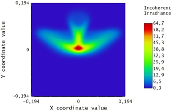
Figure 24.
Spot on a receiver with a 194-mm radius for the winter solstice.
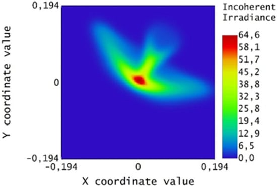
Figure 25.
Spot of the paraboloid rotated by 30° (corresponding to 10 o’clock or 14 o’clock).
In a previous study, using combined optical and mechanical simulations, Ruelas et al. [11] conclude that “When performing a ray tracing simulation and analyses of the geometric of solar image in the receiver for comparison with the infrared image, we found that the more suitable geometry for the receiver has an elliptical form”. However, they do not consider that during the day the reflector is rotated, so the image also rotates around the center of the receiver. Hence, the optimal shape is circular, with a radius corresponding to the major dimension (three times the maximum RMS value of the spot size).
The size of the beam also affects the concentration ratio of the system.
Given that the aperture of the receiver is often determined by the configuration at the equinox, it appears that the actual losses at the solstices are greater than estimated. An accurate analysis of the dimensions of the concentrated beam, even for different positions (up to the solstices), can lead to considering the use of larger dimensions for the aperture and, possibly, also for the receiver. However, this causes the concentration ratio to decrease. For applications that instead require a certain concentration ratio, the option of adding a secondary optic should be considered. In this case, the operation is not easy; since this secondary optic is close to the focus of the system, it must withstand considerable power densities, even if it is hit only by the external part of the concentrated beam (in green, in Figure 24 and Figure 25).
6. Conclusions
The proposed optical approach to the design of a Scheffler-type concentrator employs commercial raytracing software, while most of the design methods found in the literature are based on mechanical studies. Combining CAD3D results with raytracing simulations, the presented analyses calculate the light distribution created by a Scheffler reflector on a receiver.
Among the various type of concentrators developed for the small thermal applications, the Scheffler type concentrator seems especially suitable for systems with fixed receivers. To optimize its performance in collecting sunlight it is necessary to mechanically deform a Scheffler reflector. The proposed raytracing analyses can predict the shape of the light spot on the receiver as a function of the deformations applied to the mirror.
From the optical point of view, this implies that the image produced by the deformed collector is distorted and contains aberrations. As evidenced by the raytracing analyses presented, the size of the spot on the receiver enlarges and the concentration ratio decreases. The root–mean–square values of the spot sizes at the equinox are 7.37 mm × 7.37 mm, so a receiver with a radius of 18.43 mm covers the entire beam. The deformation at the winter solstice causes RMS values of the spot sizes of 64.58 mm × 34.07 mm, so the radius of the receiver is 161.44 mm, which is 8.76 times the value of the equinox case.
In order to evaluate the correct size of the receiver, two software tools have to be utilized: the first one for the reproduction of the physical components and the mechanical deformation, and the second one for the raytracing study of the optical system (especially referring to the size and shape of the spot on the receiver). The combination of these two software tools is particularly crucial in the first bending action—bending, which is the only deformation that can be optimized. The second bending, which leads to the real final shape of the paraboloid, when determined by the length of the mechanical support, is not, then, optimizable. For the examined Scheffler concentrator [2] the numerical values quantifying the mechanical deformation are: rotation −11.75°, first bending 5.0°, second bending −9.0°, for summer solstice and rotation 11.75°, first bending 5.0°, second bending −8.3°, for the winter solstice.
The knowledge of the optimal positions of the points where the pressure for the deformation has to be applied allows the implementation of an automatic mechanical movement.
The results of the simulations are here obtained for an ideal continuous mirror, while, in practice, the Scheffler concentrators are manufactured by a mosaic of flat elementary mirrors. Therefore, the power is overestimated, and the spot is smaller than that obtained by a faceted mirror. When the spot is obtained by a faceted reflector made of flat mirrors, the size of the image produced by the elementary mirror depends on the dimension of the mirror and on its distance from the target only.
The transition to a mosaic mirror is strongly influenced by the sizing of the receiver; in fact, the minimum spot size is determined by the size of the elementary mirror.
The results show that, to have high concentration, a secondary concentrator is mandatory to reduce the spot size on the receiver.
The simulations permit also to highlight a limitation of the deformation method: the fixed length of the bars limits the reduction of the beam in the X direction. For some applications, the bars could be replaced with pistons or other mechanical tools, which would help to further reduce the spot size.
In conclusion, the presented study, which combines mechanical simulation and optical raytracing analyses, sets a method to design optical components in order to reduce the losses in a thermal collector employing a Scheffler concentrator.
Author Contributions
Conceptualization, D.F. and F.F.; methodology, F.F. and F.T.; software, D.F., F.F., F.T.; validation, P.S. and D.J.; writing—original draft preparation, D.F., P.S., F.F., F.T.; writing—review and editing, P.S. and D.J.; visualization, D.F., F.F., F.T.; supervision, D.F. and F.F. All authors have read and agreed to the published version of the manuscript.
Funding
This research received no external funding.
Institutional Review Board Statement
Not applicable.
Informed Consent Statement
Not applicable.
Conflicts of Interest
The authors declare no conflict of interest.
References
- Ruelas, J.; Velasquez, N.; Beltran, R. Opto–geometric performance of fixed-focus solar concentrators. Sol. Energy 2017, 141, 303–310. [Google Scholar] [CrossRef]
- Munir, A.; Hensel, O.; Scheffler, W. Design principle and calculations of a Scheffler fixed focus concentrator for medium temperature applications. Sol. Energy 2010, 84, 1490–1502. [Google Scholar] [CrossRef]
- Junare, S.S.; Zamre, S.V.; Aware, M.M. Scheffler Dish and its Applications. In Proceedings of the International Conference on Emanations in Modern Engineering Science and Management (ICEMESM-2017), Nagpur, Maharashtra, India, 25–26 March 2017; Volume 5, pp. 1–9, ISSN 2321-8169. Available online: http://www.ijritcc.org (accessed on 14 October 2021).
- Rapp, J.; Schwartz, P. Construction and Improvement of a Scheffler Reflector and Thermal Storage Device; Cal Poly Physics Insitute, California Polytechnic State University: San Luis Obispo, CA, USA, 2010; Available online: https://digitalcommons.calpoly.edu/cgi/viewcontent.cgi?article=1023&context=physsp (accessed on 14 October 2021).
- Reddy, D.S.; Khan, M.K. Design and ray tracing of multifaceted Scheffler reflector with novel crossbars. Sol. Energy 2019, 185, 363–373. [Google Scholar] [CrossRef]
- Munir, A.; Hensel, O.; Scheffler, W.; Hoedt, H.; Amjad, W.; Ghafoor, A. Design, Development and Experimental Results of a Solar Distillery for the Essential Oils Extraction from Medicinal and Aromatic Plants. Sol. Energy 2014, 108, 548–559. [Google Scholar] [CrossRef]
- Panchal, H.; Patel, J.; Parmar, K.; Patel, M. Different applications of Scheffler reflector for renewable energy: A comprehensive review. Int. J. Ambient Energy 2020, 41, 716–728. [Google Scholar] [CrossRef]
- Islam, Q.U.; Khozaei, F. The Review of Studies on Scheffler Solar Reflectors. In Intelligent Techniques and Applications in Science and Technology; Dawn, S., Balas, V., Esposito, A., Gope, S., Eds.; Springer Nature: Cham, Switzerland, 2020; Volume 12, pp. 589–595. ISBN 978-3-030-42363-6. [Google Scholar] [CrossRef]
- Vyas, A.; Sodha, D.; Chanani, J.; Fataniya, J.; Patel, P.; Patel, D.; Basak, D. Estimation of Captured Energy Using Novel Receiver for Scheffler Dish Solar Collector. J. Therm. Energy Syst. 2018, 3, 44–52. [Google Scholar] [CrossRef]
- Malwad, D.; Tungikar, V. Experimental performance analysis of an improved receiver for Scheffler solar concentrator. SN Appl. Sci. 2020, 2, 1992. [Google Scholar] [CrossRef]
- Ruelas, J.; Pando, G.; Lucero, B.; Tzab, J. Ray Tracing Study to Determine the Characteristics of the Solar Image in the Receiver for a Scheffler-Type Solar Concentrator Coupled with a Stirling Engine. Energy Procedia 2014, 57, 2858–2866. [Google Scholar] [CrossRef] [Green Version]
- Kumar, S.; Shendage, D.J.; Doke, P.; Kedare, S.B.; Bapat, S.L. Numerical Investigation of Convective Heat Loss from Upward Facing Cavity Receivers of Different Shapes at Different Inclinations and Temperatures. J. Energy Environ. Sustain. 2019, 8, 7–11. [Google Scholar] [CrossRef]
Publisher’s Note: MDPI stays neutral with regard to jurisdictional claims in published maps and institutional affiliations. |
© 2021 by the authors. Licensee MDPI, Basel, Switzerland. This article is an open access article distributed under the terms and conditions of the Creative Commons Attribution (CC BY) license (https://creativecommons.org/licenses/by/4.0/).