Open-Circuit Fault-Tolerant Strategy for Interleaved Boost Converters via Filippov Method

Abstract

Interleaved converters use an increased number of power electronics switches; this may subsequently affect their reliability. However, this is an opportunity to develop fault-tolerant strategies to improve their reliability and to ensure continuity of service. This is why we herein propose, for the first time, a mathematical function to simultaneously model the healthy and faulty conditions of each switch, thus enabling a unique model of the system. This model is then used in an original fault-tolerant strategy based upon the peak current control with slope compensation. This method not only extends the stable range of the load variation but also ensures the stability in faulty conditions. Finally, the simulation results validate its effectiveness and confirm the theoretical analysis.

1. Introduction

Interleaved converters are applied to various applications as solar energy [1,2,3,4], fuel cell [5,6], power factor correction [7], automotive [8,9,10], and dc–dc switched-mode power converters [11], including wind systems [12,13]. The converters reliability is a great concern in such embedded applications. According to [14], the converters are sensitive to a failure of their semiconductor devices, which are their most fragile components. The system performance may be deteriorated by an open-circuit [5,15,16,17,18,19,20] or short-circuit [17] fault, which can be diagnosed through the inductive current measurement. Therefore, the converters with switch faults [4,21] are thoroughly studied.

Interleaving power converters allows to increase power density, voltage levels, and to improve EMC performances. The main advantages of interleaved [5,16,20] dc–dc converters are the reduction of current and voltage ripples and the improvement of the high current control, compared to single-phase boost converters. Moreover, the passive components (inductor and capacitor) volume and mass are reduced. A computer-aided design methodology is introduced to design a power converter which determines the number of phases to optimize cost, size, and weight of the converter [10]. References [10,13,22,23] are limited to three, four, and five paralleled converters branches. Later, in 2004, Garcia analyzed an interleaved dc–dc converter with 16 and 32 phases [9].

In general, a dc–dc converter is a dynamical system with differential equations having discontinuous right-hand sides. The converter can exhibit unpredictable phenomena such as bifurcations and chaotic operations caused by the passage switching between several subsystems. The study of periodic orbit stability requires special techniques. The average technique [24,25] is used to obtain the stability operation for the small switching period and to eliminate the nonlinear effects that occur on slow time scales. It destroys all the details about high clock frequency. Another widely used approach, which preserves the nonlinear effects, is the iterated map of the converter model. Reference [25] applies this technique and obtains a discrete observation at every clock’s instant state, namely the Poincaré map. This nonlinear map is obtained with a local linearization at a fixed point. However, in many converters, such a map cannot be derived in a closed form because of the transcendental form of the involved equations.

In later work, the authors [26,27] used the Filippov approach as an alternative method to obtain the Jacobian of the Poincaré map. The Filippov method led to many papers in several kinds of mechanical and electrical applications, including systems with velocity reversals and viscoelastic supports [28,29], and buck, boost, and Cuk converters [26,27,30]. In the literature, this approach has also been applied to general piecewise dynamical systems [31,32,33]. The Filippov method describes the stability of periodic orbits by the monodromy matrix over a complete cycle [30,34]. This method treats each switching instant separately; the overall analysis is simpler than the conventional Poincaré map. The Filippov approach is much easier to obtain the eigenvalues of the monodromy matrix and to predict the converter stability. The conventional Poincaré map Jacobian approach and the Filippov method lead to the same results.

In the field of power electronics, the analysis of a single phase converter through Filippov method is now well established. In 2017, Wu [35] proposed the Filippov approach to investigate nonlinear phenomena of an interleaved boost converter. In this work, the authors developed a new technique to control the nonlinearity in an interleaved boost converter: the peak current control with slope compensation. Thus, with this control loop, the input voltage parameter range can be extended so that the 1T-period operation of the converter remains stable. A number of modifications of control strategies have been proposed, some aimed at increasing the accuracy of the stability and the range of the parameter variation. Earlier, another widely used supervising controller was introduced to study the system operation change from unstable periodic orbits to a periodic orbits. The Ott–Grebogi–Yorke approach [36] is a well-known chaos control method, for which no analytical knowledge of the system dynamics is required. Recently, delayed feedback control methods were developed by [37,38] to stabilize the unstable periodic orbits. In the latter works, the authors develop other techniques such as as the filter-based non-invasive method, predictive control, frequency-domain, and Filippov’s method with slope compensation approaches to impose a stable periodic orbit.

The influence of slope parameter cannot be investigated theoretically in most state-space-averaging-based methods: no relationship between the margin of stable operation and the slope parameter can be determined. The addition of a small-amplitude sinusoid to the ramp waveform is an alternative way to influence the saltation matrix, but it has very little influence on the switching instant, and hence on the normal operation of the converter. As the time derivative of the switching function contains a cosine term which attains maximum value at the switching instant, this term is affected. This significantly alters the saltation matrix and offers a handle in increasing the stability margin. In this approach, the compensation ramp directly affects the saltation matrix by influencing the time derivative of the switching function, and through that, the monodromy matrix. This matrix includes comprehensive information on the converter’s parameters and the control loop. This method is an alternative to other existing methods. It also offers a deeper insight into the way the limit cycles lose their stability: it has the effect of pushing the eigenvalues inside the unit circle. From this analysis, an advanced control algorithm is developed to guarantee the satisfactory performance of the converter, avoiding nonlinear behaviors such as fast- and slow-scale bifurcations.

Our goal herein is to study the stability of a three-phase interleaved boost converter in healthy and open-circuit faulty conditions. This paper introduces a function which enables to distinguish between a defective open-circuit and an healthy open-circuit operation. First of all, the proposed function is universally applicable to any interleaved or single-phase dc–dc converters. More interesting, a single monodromy matrix is defined to understand and analyze the stability of the boost converters under different operating conditions, via Filippov’s method. This matrix contains system information, including the converter parameters, the coefficients of the feedback loop controller, and the functions. In this paper, the Neimark bifurcation occurs where the complex conjugate eigenvalues are outside the unit circle equation, when the fixed point loses stability under healthy condition. To investigate such an event, it is necessary to compute the Floquet multiplier of the 1T-period orbit, which indicates the partial instability of the system with healthy conditions and a total instability with open-circuit fault for several loads and constant input voltage. Therefore, based on this premise, the same peak current control with slope compensation as above is used to ensure a fault-tolerance operation under the load variation of interleaved dc–dc converters and to increase the range of parameters (such as input voltage or load) over which the converter remains stable. This method is an alternative to other existing methods. It also offers a deeper insight into the way the limit cycles lose their stability: it has the effect of pushing the eigenvalues inside the unit circle. Moreover, we compare our theoretical results with the ones obtained by simulation.

The main aspects of this paper are as follows: a function to model the healthy and open-circuit conditions is introduced to model a three-phase interleaved boost converter in Section 2. In Section 3, this mathematical model (under different operating modes) is applied simultaneously to each switch, thus enabling a unique model of the system. Then, in Section 4, the saltation matrices and the monodromy matrix are detailed, followed by the identification of the duty cycle in Section 5, which allows the localization of the 1T-period limit cycle to predict the converter stability. Section 6 presents a control strategy with the slope compensation in order to increase the stability of the boost converter for several loads, and a constant input voltage. We end with a conclusion in Section 7.

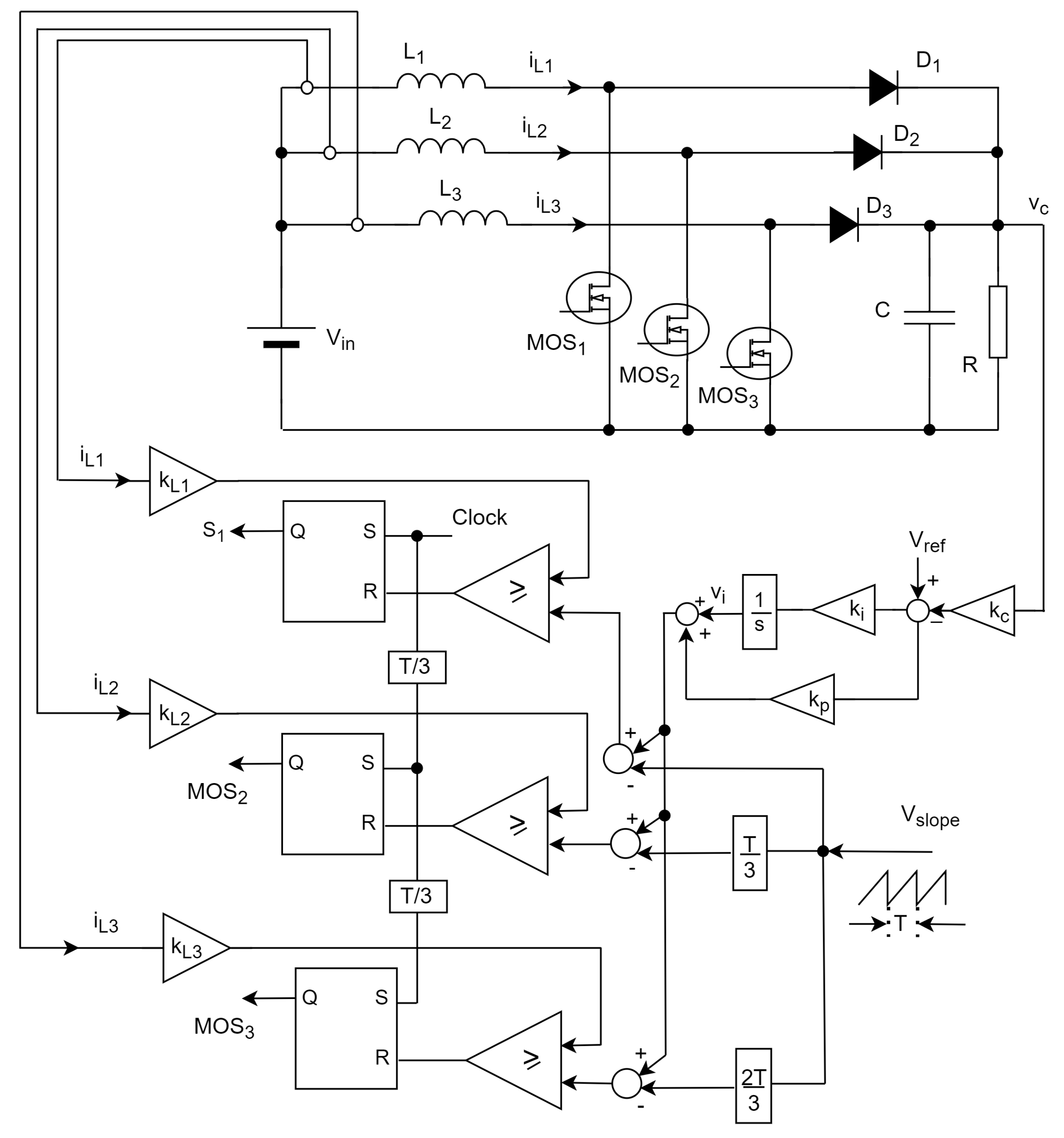
2. The Interleaved Boost Converter with Healthy and One Open-Circuit Faulty Condition

In this paper, our study is focused on a three-phase interleaved boost converter, which consists of three independent boost branches. Let us consider the circuit of Figure 1 presenting its topology. We assume that the circuit parameters of each branch are exactly the same for the three levels connected in parallel with the current phase shifted by $\pi /3$, as shown Figure 2 [35]. The parameters of the converter (the inductance, capacity, load resistance, clock frequency, input value, ...) are chosen to obtain the desired voltage ratio. The design of each branch satisfies the symmetry relation. Therefore, $L_1=L_2=L_3=L$ and $k_{L1}=k_{L2}=k_{L3}=k_L$.

In addition, it is very important to have a control voltage loop [30] in order to keep the output voltage constant. The control strategies of the interleaved boost converter are voltage mode control and a peak current control. The circuit consists of inductances $L_1$, $L_2$, and $L_3$, diodes $D_1$, $D_2$, and $D_3$, switches $MO{S}_1$, $MO{S}_2$, and $MO{S}_3$, capacitance C, and the load R. $k_i$ and $k_p$ represent the gains of the PI controller. The feedback consists of a gain $k_c$ applied to the output voltage $v_c$ and a gain $k_L$ applied to the inductor currents $i_{L1}$, $i_{L2}$, and $i_{L3}$. The output voltage $v_c$ follows the reference signal $V_{ref}$ equation, the required output voltage. The converter itself is governed by five sets of linear differential equations related to the capacitor voltage $v_c$, the inductor currents $i_{L1}$, $i_{L2}$, and $i_{L3}$, and the output of the integrator in the feedback loop $v_i$. All these variables are considered as state variables of the system noted $x_1$, $x_2$, $x_3$, $x_4$, and $x_5$.

The branches are driven by gate pulses: the controllable devices ($MO{S}_1$, $MO{S}_2$, $MO{S}_3$) are switched at the same frequency with a $T/3$ phase difference. Each branch has two modes, when the switch is either $ON$ or $OFF$. Typical failures are open-circuit or short-circuit of $MO{S}_i$ ($i=1,2,3$) or no $RS$ latch trigger pulse output. We shall only consider the MOS open-circuit fault equation during the $ON$ mode.

In order to determine the mathematical model of the healthy and faulty conditions, a binary function $h_i$ (i = 1, 2, 3) is defined as follows:

$$h_i=\left\{\begin{array}{c}1\mathrm{if}\mathrm{the}\mathrm{switching}MO{S}_i\mathrm{device}\mathrm{is}\mathrm{healthy}\hfill \\ 0\mathrm{open}-\mathrm{circuit}\mathrm{fault}\mathrm{of}\mathrm{the}MO{S}_i\mathrm{device}(\mathrm{i}=1,2,3).\hfill \end{array}\right.$$

(1)

Let us consider that an $MO{S}_i$ is turned $ON$ (i = 1 or 2 or 3) and the others, $MO{S}_j$ and $MO{S}_m$ ($j\ne i\ne m$), are turned $OFF$. If the $MO{S}_i$ is healthy, then diode $D_i$ is reverse-biased and is $OFF$. Consequently, the input voltage (applied across the inductor $L_i$) becomes $u_{Li}=V_{in}$. The currents through capacitance C and load R are provided by the inductor currents $i_{Lj}$ and $i_{Lm}$: $i_C+i_R=i_{Lj}+i_{Lm}$ ($j\ne i\ne m$). If an open-circuit fault of the $MO{S}_i$ occurs when this one is turned $ON$, the voltage across $L_i$ is $u_{Li}=V_{in}-x_1$ (i = 1 or 2 or 3). In this case, the currents through capacitance C and load R are $i_C+i_R=i_{Lj}+i_{Li}+i_{Lm}$ ($j\ne i\ne m$). Consequently, a mathematical model is able to represent both the healthy and faulty conditions of the $MO{S}_i$ which can be defined by

$$V_{in}=u_{Li}+\overline{h_i}·x_{1}i=1\mathrm{or}2\mathrm{or}3;$$

(2)

$$i_C+i_R=i_{Lj}+\overline{h_i}·i_{Li}+i_{Lm},j\ne i\mathrm{and}m\ne j.$$

(3)

3. Mathematical Model of the Boost Converter under Several Operating Modes

The mathematical model [35] of the interleaved boost converter depends on the state of the switching devices $MO{S}_1$, $MO{S}_2$, and $MO{S}_3$. However, the converter evolves in six modes during a period, when the system is T-periodical.

3.1. Mode $ON$ $OFF$ $ON$ $[0\le t\le dT-T/3]$

This mode occurs when $MO{S}_1$ is turned ON, $MO{S}_2$ is in $OFF$-state, and $MO{S}_3$ is in $ON$-state. The current $i_{L1}$ flows through $MO{S}_1$ and increases linearly from its initial value, as shown in Figure 2. The current $i_{L3}$ through $MO{S}_3$ also increases linearly and $i_{L2}$, the current of $L_2$, flows through $D_2$, C, and R. In case of open-circuit faults of $MO{S}_1$ and $MO{S}_3$ too, the currents $i_{L1}$ and $i_{L3}$ are added to $i_{L2}$. The capacitor and load currents are described by

$$i_C+i_R=\overline{h_1}·i_{L1}+i_{L2}+\overline{h_3}·i_{L3},\frac{d{x}_1}{dt}=-\frac{1}{RC}·x_1+\frac{\overline{h_1}}{C}·x_2+\frac{1}{C}·x_3+\frac{\overline{h_3}}{C}·x_4.$$

(4)

The voltages across $L_1$, $L_2$, $L_3$ and the derivatives of $i_{L1}$, $i_{L2}$, $i_{L3}$ can be expressed [26,27] as follows:

$$\begin{array}{ccc}\hfill & V_{in}=u_{L1}+\overline{h_1}·x_1\hfill & \hfill \frac{d{x}_2}{dt}=-\frac{\overline{h_1}}{L}·x_1+\frac{V_{in}}{L},\\ \hfill & V_{in}=u_{L2}+x_1\hfill & \hfill \frac{d{x}_3}{dt}=-\frac{1}{L}·x_1+\frac{V_{in}}{L},\\ \hfill & V_{in}=u_{L3}+\overline{h_3}·x_1\hfill & \hfill \frac{d{x}_4}{dt}=-\frac{\overline{h_3}}{L}·x_1+\frac{V_{in}}{L}.\end{array}$$

(5)

$v_i$, the control voltage of the integrator and its derivative $\frac{d{x}_5}{dt}$ are given by the following equations:

$$v_i=\frac{k_i}{s}\left(V_{ref}-k_c·x_1\right),\frac{d{x}_5}{dt}=-k_i{k}_c·x_1+k_i·V_{ref}.$$

(6)

The evolutions of the state variables in Mode $ON$$OFF$ $ON$ during $[0\le t\le dT-T/3]$ can be described by the following matrix equations and the right-side state equations as:

$$A_1=\left[\begin{array}{ccccc}-\frac{1}{RC}& \frac{{\overline{h}}_1}{C}& \frac{1}{C}& \frac{{\overline{h}}_3}{C}& 0\\ \\ -\frac{{\overline{h}}_1}{L}& 0& 0& 0& 0\\ \\ -\frac{1}{L}& 0& 0& 0& 0\\ \\ -\frac{{\overline{h}}_3}{L}& 0& 0& 0& 0\\ \\ -k_i{k}_c& 0& 0& 0& 0\end{array}\right],B_1=\left[\begin{array}{cc}0& 0\\ \\ \frac{1}{L}& 0\\ \\ \frac{1}{L}& 0\\ \\ \frac{1}{L}& 0\\ \\ 0& k_i\end{array}\right].f_1=\left[\begin{array}{c}-\frac{1}{RC}{x}_1+\frac{{\overline{h}}_1}{C}{x}_2+\frac{1}{C}{x}_3+\frac{{\overline{h}}_3}{C}{x}_4\\ \\ -\frac{{\overline{h}}_1}{L}·x_1+\frac{1}{L}·V_{in}\\ \\ -\frac{1}{L}·x_1+\frac{1}{L}·V_{in}\\ \\ -\frac{{\overline{h}}_3}{L}·x_1+\frac{1}{L}·V_{in}\\ \\ -k_i{k}_c·x_1+k_i·V_{in}\end{array}\right]$$

(7)

3.2. Mode $ON$ $OFF$ $OFF$ $[dT-T/3\le t\le T/3]$

This mode occurs when $MO{S}_3$ is turned $OFF$ and when $i_{L3}$ decreases linearly from the peak current according to the control strategy. $MO{S}_1$ is in $ON$-state, so the current $i_{L1}$ through $MO{S}_1$ continues to increase linearly. $MO{S}_2$ is in $OFF$-state and $i_{L2}$ decreases linearly until the occurrence of the clock pulse at $T/3$. The capacitor and load currents are described by

$$i_C+i_R=\overline{h_1}·i_{L1}+i_{L2}+i_{L3},\frac{d{x}_1}{dt}=-\frac{1}{RC}·x_1+\frac{\overline{h_1}}{C}·x_2+\frac{1}{C}·x_3+\frac{1}{C}·x_4,$$

(8)

The voltages across $L_1$, $L_2$, $L_3$ and the derivatives of $i_{L1}$, $i_{L2}$, $i_{L3}$ can be calculated as follows:

$$\begin{array}{ccc}\hfill & V_{in}=u_{L1}+\overline{h_1}·x_1\hfill & \hfill \frac{d{x}_2}{dt}=-\frac{\overline{h_1}}{L}·x_1+\frac{V_{in}}{L},\\ \hfill & V_{in}=u_{L2}+x_1\hfill & \hfill \frac{d{x}_3}{dt}=-\frac{1}{L}·x_1+\frac{V_{in}}{L},\\ \hfill & V_{in}=u_{L3}+x_1\hfill & \hfill \frac{d{x}_4}{dt}=-\frac{1}{L}·x_1+\frac{V_{in}}{L}.\end{array}$$

(9)

$v_i$, the control voltage of the integrator, as well as $\frac{d{x}_5}{dt}$, are given in Equation (6). The evolution of the state variables during this interval can be described by the following matrix equations and the right-side state equations:

$$A_2=\left[\begin{array}{ccccc}-\frac{1}{RC}& \frac{{\overline{h}}_1}{C}& \frac{1}{C}& \frac{1}{C}& 0\\ \\ -\frac{{\overline{h}}_1}{L}& 0& 0& 0& 0\\ \\ -\frac{1}{L}& 0& 0& 0& 0\\ \\ -\frac{1}{L}& 0& 0& 0& 0\\ \\ -k_i{k}_c& 0& 0& 0& 0\end{array}\right],B_2=B_1,f_2=\left[\begin{array}{c}-\frac{1}{RC}{x}_1+\frac{{\overline{h}}_1}{C}{x}_2+\frac{1}{C}{x}_3+\frac{1}{C}{x}_4\\ \\ -\frac{{\overline{h}}_1}{L}·x_1+\frac{1}{L}·V_{in}\\ \\ -\frac{1}{L}·x_1+\frac{1}{L}·V_{in}\\ \\ -\frac{1}{L}·x_1+\frac{1}{L}·V_{in}\\ \\ -k_i{k}_c·x_1+k_i·V_{in}\end{array}\right].$$

(10)

3.3. Mode $ON$ $ON$ $OFF$ $[T/3\le t\le dT]$

$MO{S}_2$ is turned ON due to the impulse clock, $MO{S}_1$ is in $ON$-state, and $MO{S}_3$ is in $OFF$-state. The current $i_{L1}$ through $MO{S}_1$ continues to increase linearly until the peak current, according to the control strategy. In addition, $i_{L2}$ increases linearly and $i_{L3}$ also continues to decrease. Similarly, the capacitor current and the voltages across $L_1$, $L_2$, $L_3$ are described by

$$i_C+i_R=\overline{h_1}·i_{L1}+i_{L2}+i_{L3},\frac{d{x}_1}{dt}=-\frac{1}{RC}·x_1+\frac{\overline{h_1}}{C}·x_2+\frac{1}{C}·x_3+\frac{1}{C}·x_4,$$

(11)

and

$$\begin{array}{ccc}\hfill & V_{in}=u_{L1}+\overline{h_1}·x_1\hfill & \hfill \frac{d{x}_2}{dt}=-\frac{\overline{h_1}}{L}·x_1+\frac{V_{in}}{L},\\ \hfill & V_{in}=u_{L2}+x_1\hfill & \hfill \frac{d{x}_3}{dt}=-\frac{1}{L}·x_1+\frac{V_{in}}{L},\\ \hfill & V_{in}=u_{L3}+\overline{h_3}·x_1\hfill & \hfill \frac{d{x}_4}{dt}=-\frac{\overline{h_3}}{L}·x_1+\frac{V_{in}}{L}.\end{array}$$

(12)

Equation (6) is still available to define the control voltage of the integrator $v_i$ and its derivative. The evolution of the state variables in Mode $ON$ $OFF$ $OFF$ during $[T/3\le t\le dT]$ can be described as

$$A_3=\left[\begin{array}{ccccc}-\frac{1}{RC}& \frac{{\overline{h}}_1}{C}& \frac{{\overline{h}}_2}{C}& \frac{1}{C}& 0\\ \\ -\frac{{\overline{h}}_1}{L}& 0& 0& 0& 0\\ \\ -\frac{{\overline{h}}_2}{L}& 0& 0& 0& 0\\ \\ -\frac{1}{L}& 0& 0& 0& 0\\ \\ -k_i{k}_c& 0& 0& 0& 0\end{array}\right],B_3=B_1,f_3=\left[\begin{array}{c}-\frac{1}{RC}{x}_1+\frac{{\overline{h}}_1}{C}{x}_2+\frac{{\overline{h}}_2}{C}{x}_3+\frac{1}{C}{x}_4\\ \\ -\frac{{\overline{h}}_1}{L}·x_1+\frac{1}{L}·V_{in}\\ \\ -\frac{{\overline{h}}_2}{L}·x_1+\frac{1}{L}·V_{in}\\ \\ -\frac{1}{L}·x_1+\frac{1}{L}·V_{in}\\ \\ -k_i{k}_c·x_1+k_i·V_{in}\end{array}\right].$$

(13)

3.4. Mode $OFF$ $ON$ $OFF$ $[dT\le t\le 2T/3]$

$MO{S}_1$ is turned $OFF$, as $MO{S}_2$ is in $ON$-state and $MO{S}_3$ is in $OFF$-state. The current $i_{L1}$ through $MO{S}_1$ decreases linearly from peak current, according to the control strategy. The current $i_{L2}$ continues to increase linearly, and the current $i_{L3}$ continues to decrease linearly. Similarly, the capacitor and load current are described by

$$i_C+i_R=i_{L1}+\overline{h_2}·i_{L2}+i_{L3},\frac{d{x}_1}{dt}=-\frac{1}{RC}·x_1+\frac{1}{C}·x_2+\frac{\overline{h_2}·}{C}·x_3+\frac{1}{C}·x_4.$$

(14)

The voltages across $L_1$, $L_2$, $L_3$ and the derivatives of $i_{L1}$, $i_{L2}$, $i_{L3}$ can be expressed as follows:

$$\begin{array}{ccc}\hfill & V_{in}=u_{L1}+x_1\hfill & \hfill \frac{d{x}_2}{dt}=-\frac{1}{L}·x_1+\frac{V_{in}}{L},\\ \hfill & V_{in}=u_{L2}+\overline{h_2}·x_1\hfill & \hfill \frac{d{x}_3}{dt}=-\frac{\overline{h_2}}{L}·x_1+\frac{V_{in}}{L},\\ \hfill & V_{in}=u_{L3}+x_1\hfill & \hfill \frac{d{x}_4}{dt}=-\frac{1}{L}·x_1+\frac{V_{in}}{L}.\end{array}$$

(15)

The control voltage $v_i$ obtained from the output of the integrator and its derivative $\frac{d{x}_5}{dt}$ are as in Equation (6). During $[dT\le t\le 2T/3]$ intervals, the matrix form of the state equations are

$$A_4=\left[\begin{array}{ccccc}-\frac{1}{RC}& \frac{1}{C}& \frac{{\overline{h}}_2}{C}& \frac{1}{C}& 0\\ \\ -\frac{1}{L}& 0& 0& 0& 0\\ \\ -\frac{{\overline{h}}_2}{L}& 0& 0& 0& 0\\ \\ -\frac{1}{L}& 0& 0& 0& 0\\ \\ -k_i{k}_c& 0& 0& 0& 0\end{array}\right],B_4=B_1,f_4=\left[\begin{array}{c}-\frac{1}{RC}{x}_1+\frac{1}{C}{x}_2+\frac{{\overline{h}}_2}{C}{x}_3+\frac{1}{C}{x}_4\\ \\ -\frac{1}{L}·x_1+\frac{1}{L}·V_{in}\\ \\ -\frac{{\overline{h}}_2}{L}·x_1+\frac{1}{L}·V_{in}\\ \\ -\frac{1}{L}·x_1+\frac{1}{L}·V_{in}\\ \\ -k_i{k}_c·x_1+k_i·V_{in}\end{array}\right].$$

(16)

3.5. Mode $OFF$ $ON$ $ON$ $[2T/3\le t\le dT+T/3]$

$MO{S}_1$ is in $OFF$-state, $MO{S}_2$ is in $ON$-state, and $MO{S}_3$ is turned to $ON$-state. The current $i_{L1}$ through $MO{S}_1$ continues to decrease linearly. The current $i_{L2}$ increases linearly until the peak current, according to the control strategy. The current $i_{L3}$ begins to increase after the pulse clock at $2T/3$ time. Similarly, the capacitor and load current are described by

$$i_C+i_R=i_{L1}+\overline{h_2}·i_{L2}+\overline{h_3}·i_{L3},\frac{d{x}_1}{dt}=-\frac{1}{RC}·x_1+\frac{1}{C}·x_2+\frac{\overline{h_2}}{C}·x_3+\frac{\overline{h_3}}{C}·x_4.$$

(17)

The voltages across $L_1$, $L_2$, $L_3$ and the derivatives of $i_{L1}$, $i_{L2}$, $i_{L3}$ can be calculated as follows:

$$\begin{array}{ccc}\hfill & V_{in}=u_{L1}+x_1\hfill & \hfill \frac{d{x}_2}{dt}=-\frac{1}{L}·x_1+\frac{V_{in}}{L},\\ \hfill & V_{in}=u_{L2}+\overline{h_2}·x_1\hfill & \hfill \frac{d{x}_3}{dt}=-\frac{\overline{h_2}}{L}·x_1+\frac{V_{in}}{L},\\ \hfill & V_{in}=u_{L3}+\overline{h_3}·x_1\hfill & \hfill \frac{d{x}_4}{dt}=-\frac{\overline{h_3}}{L}·x_1+\frac{V_{in}}{L}.\end{array}$$

(18)

Equation (6) is still available to define the control voltage of integrator $v_i$ and its derivative $\frac{d{x}_5}{dt}$. The evolutions of the state variables in Mode $OFF$ $ON$ $ON$ during $[2T/3\le t\le dT+T/3]$ can be described by

$$A_5=\left[\begin{array}{ccccc}-\frac{1}{RC}& \frac{1}{C}& \frac{{\overline{h}}_2}{C}& \frac{{\overline{h}}_3}{C}& 0\\ \\ -\frac{1}{L}& 0& 0& 0& 0\\ \\ -\frac{{\overline{h}}_2}{L}& 0& 0& 0& 0\\ \\ -\frac{{\overline{h}}_3}{L}& 0& 0& 0& 0\\ \\ -k_i{k}_c& 0& 0& 0& 0\end{array}\right],B_5=B_1,f_5=\left[\begin{array}{c}-\frac{1}{RC}{x}_1+\frac{1}{C}{x}_2+\frac{{\overline{h}}_2}{C}{x}_3+\frac{{\overline{h}}_3}{C}{x}_4\\ \\ -\frac{1}{L}·x_1+\frac{1}{L}·V_{in}\\ \\ -\frac{{\overline{h}}_2}{L}·x_1+\frac{1}{L}·V_{in}\\ \\ -\frac{{\overline{h}}_3}{L}·x_1+\frac{1}{L}·V_{in}\\ \\ -k_i{k}_c·x_1+k_i·V_{in}\end{array}\right].$$

(19)

3.6. Mode $OFF$ $OFF$ $ON$ $[dT+T/3\le t\le T]$

For this last configuration, $MO{S}_1$ is in $OFF$-state, $MO{S}_2$ is turned $OFF$, and $MO{S}_3$ is in $ON$-state. The current $i_{L1}$ through $MO{S}_1$ continues to decrease linearly until the next pulse clock arrives. The current $i_{L2}$ begins to decrease linearly, and the current $i_{L3}$ continues to increase linearly. Similarly, the capacitor and load current are described by

$$i_C+i_R=i_{L1}+i_{L2}+\overline{h_3}·i_{L3},\frac{d{x}_1}{dt}=-\frac{1}{RC}·x_1+\frac{1}{C}·x_2+\frac{1}{C}·x_3+\frac{\overline{h_3}}{C}·x_4.$$

(20)

The voltages across $L_1$, $L_2$, $L_3$ and the derivatives of $i_{L1}$, $i_{L2}$, $i_{L3}$ are expressed as follows:

$$\begin{array}{ccc}\hfill & V_{in}=u_{L1}+x_1\hfill & \hfill \frac{d{x}_2}{dt}=-\frac{1}{L}·x_1+\frac{V_{in}}{L},\\ \hfill & V_{in}=u_{L2}+x_1\hfill & \hfill \frac{d{x}_3}{dt}=-\frac{1}{L}·x_1+\frac{V_{in}}{L},\\ \hfill & V_{in}=u_{L3}+\overline{h_3}·x_1\hfill & \hfill \frac{d{x}_4}{dt}=-\frac{\overline{h_3}}{L}·x_1+\frac{V_{in}}{L}.\end{array}$$

(21)

$v_i$, the control voltage of the integrator, and its derivative $\frac{d{x}_5}{dt}$ are given by Equation (6). The evolution of the state variables in Mode $OFF$ $OFF$ $ON$ during $[dT+T/3\le t\le T]$ are described by the following matrix equations and the right-hand side state equations:

$$A_6=\left[\begin{array}{ccccc}-\frac{1}{RC}& \frac{1}{C}& \frac{1}{C}& \frac{{\overline{h}}_3}{C}& 0\\ \\ -\frac{1}{L}& 0& 0& 0& 0\\ \\ -\frac{1}{L}& 0& 0& 0& 0\\ \\ -\frac{{\overline{h}}_3}{L}& 0& 0& 0& 0\\ \\ -k_i{k}_c& 0& 0& 0& 0\end{array}\right],B_6=B_1,f_6=\left[\begin{array}{c}-\frac{1}{RC}{x}_1+\frac{1}{C}{x}_2+\frac{1}{C}{x}_3+\frac{{\overline{h}}_3}{C}{x}_4\\ \\ -\frac{1}{L}·x_1+\frac{1}{L}·V_{in}\\ \\ -\frac{1}{L}·x_1+\frac{1}{L}·V_{in}\\ \\ -\frac{{\overline{h}}_3}{L}·x_1+\frac{1}{L}·V_{in}\\ \\ -k_i{k}_c·x_1+k_i·V_{in}\end{array}\right].$$

(22)

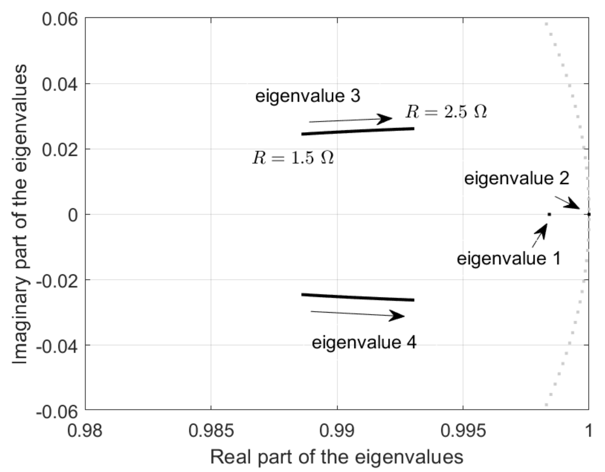
4. Saltation and Monodromy Matrices for the Interleaved Boost Converter

A linear time-invariant system is represented by the differential equation $\dot{x}\left(t\right)=f\left(x\right)$, with initial conditions. An interleaved boost converter is a the discontinuous dynamical system composed of six smooth vector fields that are separated by discontinuity boundaries. This nonlinear system, with a discontinuous right-hand side, is described by the following differential equations:

$$\dot{x}=f(t,x\left(t\right))=\left\{\begin{array}{c}{f}_1(t,x\left(t\right)),x\in V_1\hfill \\ f_2(t,x\left(t\right)),x\in V_2\hfill \\ f_3(t,x\left(t\right)),x\in V_3\hfill \\ f_4(t,x\left(t\right)),x\in V_4\hfill \\ f_5(t,x\left(t\right)),x\in V_5\hfill \\ f_6(t,x\left(t\right)),x\in V_6\hfill \end{array}\right.$$

(23)

where $f_1$ of Equation (7), $f_2$ of Equation (10), $f_3$ of Equation (13), $f_4$ of Equation (16), $f_5$ of Equation (19), and $f_6$ of Equation (22) are six smooth functions, and $x\in {\mathbb{R}}^5$. For simplicity reasons, let us consider a region of the state space ${\mathbb{R}}^5$ which splits into six subspaces [30,34]: $V_1$ and $V_2$ are separated by surface ${\mathrm{\Sigma }}_1$, $V_3$ and $V_4$ are separated by surface ${\mathrm{\Sigma }}_2$, and $V_5$ and $V_6$ are separated by surface ${\mathrm{\Sigma }}_3$, denoted by Figure 3, with:

$$\begin{array}{c}\hfill V_1=\left\{x\in {\mathbb{R}}^5:s{w}_1\left(x\left(t\right)\right)<0\right\}{V}_2=\left\{x\in {\mathbb{R}}^5:s{w}_1\left(x\left(t\right)\right)>0\right\}{\mathrm{\Sigma }}_1=\left\{x\in {\mathbb{R}}^5:s{w}_1(t,x)=0\right\},\\ \hfill V_3=\left\{x\in {\mathbb{R}}^5:s{w}_2\left(x\left(t\right)\right)<0\right\}{V}_4=\left\{x\in {\mathbb{R}}^5:s{w}_2\left(x\left(t\right)\right)>0\right\}{\mathrm{\Sigma }}_2=\left\{x\in {\mathbb{R}}^5:s{w}_2(t,x)=0\right\},\\ \hfill V_5=\left\{x\in {\mathbb{R}}^5:s{w}_3\left(x\left(t\right)\right)<0\right\}{V}_6=\left\{x\in {\mathbb{R}}^5:s{w}_3\left(x\left(t\right)\right)>0\right\}{\mathrm{\Sigma }}_3=\left\{x\in {\mathbb{R}}^5:s{w}_3(t,x)=0\right\},\end{array}$$

(24)

where $s{w}_1\left(x\left(t\right)\right)$, $s{w}_2\left(x\left(t\right)\right)$, and $s{w}_3\left(x\left(t\right)\right)$ are scalar switching functions. It is presupposed that $f_i$ ($i=\overline{1,6}$) is time continuous and discontinuous in $x_i$ ($i=\overline{1,5}$), and crosses ${\mathrm{\Sigma }}_r$ ($r=\overline{1,3}$) transversally. Discontinuous systems exhibit jumps in the evolution of the fundamental solution matrix. Filippov showed that the system of Equation (23) can be transformed into a system continuous at the switching instant [29]. Therefore, the discontinuous problem can be replaced by a continuous set-valued one as follows:

$$\dot{x}\left(t\right)=F(t,x\left(t\right))=\left\{\begin{array}{cc}{f}_i(t,x\left(t\right))\hfill & \mathrm{if}x\in V_i,\hfill \\ q{f}_i(t,x\left(t\right))+(1-q)f_{i+1}(t,x\left(t\right))\hfill & \mathrm{if}x\in {\mathrm{\Sigma }}_r,\hfill \\ f_{i+1}(t,x\left(t\right))\hfill & \mathrm{if}x\in V_{i+1}.\hfill \end{array}\right.$$

(25)

where $q\in [0,1]$, $i=\overline{1,5}$, and $r=\overline{1,3}$. Now, on ${\mathrm{\Sigma }}_r$ ($r=\overline{1,3}$), the discontinuity is replaced with the segment, which means that on ${\mathrm{\Sigma }}_r$ (r = $\overline{1,3}$), F consists of infinite number of points as shown in Figure 4. $x\left(t_i\right)$ passing from the subsystem is described by the vector $f_i$ (Equation, using the fundamental solution matrix just before the jump $t_{\mathrm{\Sigma }-}$) intersects the switching surface, and goes to the subsystem described by the vector $f_{i+1}$ (Equation, using the fundamental solution matrix just after the jump $t_{\mathrm{\Sigma }+}$).

The transition at each switching moment is described by saltation matrices which can be represented as follows:

$$S_{ii+1}={\mathbb{I}}_5+\frac{(f_{i+1}-f_i)n^T}{n_i^T{f}_i+\frac{\partial s{w}_r}{\partial t}}$$

(26)

where $f_i$ and $f_{i+1}$, $i=\overline{1,5}$ are the right-hand sides of the state equations, before and after switching, where n is a normal vector to the switching surface and $n=\nabla s{w}_r\left(x\left(t\right)\right)$.

As mentioned above, we are interested in the stability of the dynamical system, Equation (23), where the system regains a T-periodic orbit. One method to check the stability of periodic motions is to calculate, over one complete cycle $[0,T)$, the state transition matrix (monodromy matrix ${\mathrm{\Phi }}_{cycle1}$ of Figure 5) of the system and then to determine its eigenvalues. If they are inside of the unit circle, then the periodic motion is stable. For an interleaved boost converter, the state evolves through six subsystems: ON and OFF states of the $MO{S}_1$, $MO{S}_2$, and $MO{S}_3$. As we are interested in the stability of the periodic orbit exhibited by the converters, we need to calculate the state transition matrix over a whole clock cycle. The monodromy matrix must be broken into six state transition matrices of the regions before and after the switching, and five for the transition across the switching surfaces.

This matrix ${\mathrm{\Phi }}_{cycle1}$ is composed of the fundamental solution matrices where the vector field is smooth and of the saltation matrices where the vector field crosses a switching boundary ${\mathrm{\Sigma }}_r$:

$$\begin{array}{ccc}\hfill {\mathrm{\Phi }}_{cycle1}(T,0)& =& S_{61}·{\mathrm{\Phi }}_6\left(T,dT+\frac{T}{3}\right)·S_{56}·{\mathrm{\Phi }}_5\left(dT+\frac{T}{3},\frac{2T}{3}\right)·S_{45}·{\mathrm{\Phi }}_4\left(\frac{2T}{3},dT\right)·\hfill \\ & & ·S_{34}·{\mathrm{\Phi }}_3\left(dT,\frac{T}{3}\right)·S_{23}·{\mathrm{\Phi }}_2\left(\frac{T}{3},dT-\frac{T}{3}\right)·S_{12}·{\mathrm{\Phi }}_1\left(dT-\frac{T}{3},0\right)\hfill \end{array}$$

(27)

and

$${\mathrm{\Phi }}_{cycle1}(T,0)=e^{A_6\left(\frac{2T}{3}-dT\right)}·S_{56}·e^{A_5\left(dT-\frac{T}{3}\right)}·e^{A_4\left(\frac{2T}{3}-dT\right)}·cdot{S}_{34}·e^{A_3\left(dT-\frac{T}{3}\right)}·e^{A_2\left(\frac{2T}{3}-dT\right)}·S_{12}·e^{A_1\left(dT-\frac{T}{3}\right)}.$$

(28)

${\mathrm{\Phi }}_6$, ${\mathrm{\Phi }}_5$, ${\mathrm{\Phi }}_4$, ${\mathrm{\Phi }}_3$, ${\mathrm{\Phi }}_2$, and ${\mathrm{\Phi }}_1$ are fundamental solution matrices depending on $A_6$, $A_5$, $A_4$, $A_3$, $A_2$ and $A_1$. $S_{12}$, $S_{23}$, $S_{34}$, $S_{45}$, $S_{56}$, and $S_{61}$ are the saltation matrices calculated at the instants $dT-T/3$, $T/3$, $dT$, $2T/3$, $T/3+dT$, and T. The saltation matrices $S_{23}$, $S_{45}$, and $S_{61}$ are related to the switching from $OFF$ to $ON$ modes. These matrices turn out to identical matrices ${\mathbb{I}}_5$, because $s{w}_r$ ($r=\overline{1,3}$) are discontinuous at the instants ($T/3$, $2T/3$, and T), and in consequence $\partial s{w}_r$/$\partial t$ = infinite.

From the circuit topology (Figure 1), the switching functions are

$$\begin{array}{c}s{w}_1(x,t)=k_L·x_4\left(t\right)-x_5\left(t\right)+k_p·\left(k_c·x_1\left(t\right)-V_{ref}\right),\\ s{w}_2(x,t)=k_L·x_2\left(t\right)-x_5\left(t\right)+k_p·\left(k_c·x_1\left(t\right)-V_{ref}\right),\\ s{w}_3(x,t)=k_L·x_3\left(t\right)-x_5\left(t\right)+k_p·\left(k_c·x_1\left(t\right)-V_{ref}\right),\end{array}$$

(29)

and their time derivation

$$\frac{\partial s{w}_1}{\partial t}=\frac{\partial s{w}_2}{\partial t}=\frac{\partial s{w}_3}{\partial t}=0.$$

(30)

The normal vectors at the point x are given by

$$\begin{array}{c}\hfill \frac{\partial s{w}_1}{\partial x}=n_1=\left[\begin{array}{c}\frac{\partial s{w}_1}{\partial x_1}\\ \frac{\partial s{w}_1}{\partial x_2}\\ \frac{\partial s{w}_1}{\partial x_3}\\ \frac{\partial s{w}_1}{\partial x_4}\\ \frac{\partial s{w}_1}{\partial x_5}\end{array}\right]=\left[\begin{array}{c}{k}_p{k}_c\\ 0\\ 0\\ k_L\\ -1\end{array}\right],\end{array}$$

(31)

$$\begin{array}{c}\hfill \frac{\partial s{w}_2}{\partial x}=n_2=\left[\begin{array}{c}\frac{\partial s{w}_2}{\partial x_1}\\ \frac{\partial s{w}_2}{\partial x_2}\\ \frac{\partial s{w}_2}{\partial x_3}\\ \frac{\partial s{w}_2}{\partial x_4}\\ \frac{\partial s{w}_2}{\partial x_5}\end{array}\right]=\left[\begin{array}{c}{k}_p{k}_c\\ k_L\\ 0\\ 0\\ -1\end{array}\right]\end{array}$$

(32)

and

$$\begin{array}{c}\hfill \frac{\partial s{w}_3}{\partial x}=n_3=\left[\begin{array}{c}\frac{\partial s{w}_3}{\partial x_1}\\ \frac{\partial s{w}_3}{\partial x_2}\\ \frac{\partial s{w}_3}{\partial x_3}\\ \frac{\partial s{w}_3}{\partial x_4}\\ \frac{\partial s{w}_3}{\partial x_5}\end{array}\right]=\left[\begin{array}{c}{k}_p{k}_c\\ 0\\ k_L\\ 0\\ -1\end{array}\right].\end{array}$$

(33)

By substitution of Equations (7), (10), (30), and (31) into Equation (26), the saltation matrix $S_{12}$ at the moment $t=dT-\frac{T}{3}$ can be obtained in the following form:

$$\begin{array}{c}\hfill S_{12}=\left[\begin{array}{ccccc}1+\frac{(1-{\overline{h}}_3)·x_4{k}_p{k}_c}{de{n}_{12}·C}& 0& 0& \frac{(1-{\overline{h}}_3)·x_4{k}_L}{de{n}_{12}·C}& -\frac{(1-{\overline{h}}_3)·x_4}{de{n}_{12}·C}\\ 0& 1& 0& 0& 0\\ 0& 0& 1& 0& 0\\ -\frac{(1-{\overline{h}}_3)·x_1{k}_p{k}_c}{de{n}_{12}·L}& 0& 0& 1-\frac{(1-{\overline{h}}_3)·x_1{k}_L}{de{n}_{12}·L}& \frac{(1-{\overline{h}}_3)·x_1}{de{n}_{12}·L}\\ 0& 0& 0& 0& 1\end{array}\right],\end{array}$$

(34)

where

$$de{n}_{12}=\left(k_i{k}_c-\frac{k_p{k}_c}{RC}-\frac{k_L{\overline{h}}_3}{L}\right)·x_1+k_p{k}_c\frac{{\overline{h}}_1}{C}·x_2+\frac{k_p{k}_c}{C}·x_3+k_p{k}_c\frac{{\overline{h}}_3}{C}·x_4+\frac{k_L}{L}·V_{in}-k_i·V_{ref}.$$

(35)

With Equations (13), (16), (30), (32), and (26), at $t=dT$, the saltation matrix $S_{34}$ is given by

$$\begin{array}{c}\hfill S_{34}=\left[\begin{array}{ccccc}1+\frac{(1-{\overline{h}}_1)·x_2{k}_p{k}_c}{de{n}_{34}·C}& \frac{(1-{\overline{h}}_1)·x_2{k}_L}{de{n}_{34}·C}& 0& 0& -\frac{(1-{\overline{h}}_1)·x_2}{de{n}_{34}·C}\\ -\frac{(1-{\overline{h}}_1)·x_1{k}_p{k}_c}{de{n}_{34}·L}& 1-\frac{(1-{\overline{h}}_1)·x_1{k}_L}{de{n}_{34}·L}& 0& 0& \frac{(1-{\overline{h}}_1)·x_1}{de{n}_{34}·L}\\ 0& 0& 1& 0& 0\\ 0& 0& 0& 1& 0\\ 0& 0& 0& 0& 1\end{array}\right],\end{array}$$

(36)

where

$$de{n}_{34}=\left(k_i{k}_c-\frac{k_p{k}_c}{RC}-\frac{k_L{\overline{h}}_1}{L}\right)·x_1+k_p{k}_c\frac{{\overline{h}}_1}{C}·x_2+k_p{k}_c\frac{{\overline{h}}_2}{C}·x_3+\frac{k_p{k}_c}{C}·x_4+\frac{k_L}{L}·V_{in}-k_i·V_{ref}.$$

(37)

Using Equations (19), (22), (30), (33), and (26), the saltation matrix $S_{56}$ at the instant $t=dT+\frac{T}{3}$ becomes

$$\begin{array}{c}\hfill S_{56}=\left[\begin{array}{ccccc}1+\frac{(1-{\overline{h}}_2)·x_3{k}_p{k}_c}{de{n}_{56}·C}& 0& \frac{(1-{\overline{h}}_2)·x_3{k}_L}{de{n}_{56}·C}& 0& -\frac{(1-{\overline{h}}_2)·x_3}{de{n}_{56}·C}\\ 0& 1& 0& 0& 0\\ -\frac{(1-{\overline{h}}_2)·x_1{k}_p{k}_c}{de{n}_{56}·L}& 0& 1-\frac{(1-{\overline{h}}_2)·x_1{k}_L}{de{n}_{56}·L}& 0& \frac{(1-{\overline{h}}_2)·x_1}{de{n}_{56}·L}\\ 0& 0& 0& 1& 0\\ 0& 0& 0& 0& 1\end{array}\right],\end{array}$$

(38)

where

$$de{n}_{56}=\left(k_i{k}_c-\frac{k_p{k}_c}{RC}-\frac{k_L{\overline{h}}_2}{L}\right)·x_1+\frac{k_p{k}_c}{C}·x_2+k_p{k}_c\frac{{\overline{h}}_2}{C}·x_3+k_p{k}_c\frac{{\overline{h}}_3}{C}·x_4+\frac{k_L}{L}·V_{in}-k_i·V_{ref}.$$

(39)

5. Identification of Duty Cycles of the Period-1T Limit Cycle

The duty cycle d is calculated in order to locate the limit cycle for several values of the load R. When the switch occurs on the surface ${\mathrm{\Sigma }}_1$, the state vector at $t=dT-\frac{T}{3}$ is given by

$$\begin{array}{c}\hfill x(dT-T/3)=e^{A_1·(dT-T/3)}·x\left(0\right)+{\int }_0^{dT-T/3}{e}^{A_1·(dT-T/3-\tau )}·B_{1}ud\tau ={\mathrm{\Phi }}_1·x\left(0\right)+Inte{g}_1.\end{array}$$

(40)

The state vector at the clock pulse $t=T/3$ is as follows:

$$x(T/3)=e^{A_2·(2T/3-dT)}·x(dT-T/3)+{\int }_{dT-T/3}^{T/3}{e}^{A_2·(T/3-\tau )}·B_{2}ud\tau ={\mathrm{\Phi }}_2·x(dT-T/3)+Inte{g}_2.$$

(41)

At switching surface ${\mathrm{\Sigma }}_2$ for $t=dT$, the state vector can be expressed as

$$x\left(dT\right)=e^{A_3·(dT-T/3)}·x(T/3)+{\int }_{T/3}^{dT}{e}^{A_3·(dT-\tau )}·B_{3}ud\tau ={\mathrm{\Phi }}_3·x(T/3)+Inte{g}_3.$$

(42)

For the second clock pulse $t=2T/3$, the state vector is

$$x(2T/3)=e^{A_4·(2T/3-dT)}·x\left(dT\right)+{\int }_{dT}^{2T/3}{e}^{A_4·(2T/3-\tau )}·B_{4}ud\tau ={\mathrm{\Phi }}_4·x\left(dT\right)+Inte{g}_4.$$

(43)

The state vector at the switching surface ${\mathrm{\Sigma }}_3$ is given by

$$x(dT+T/3)=e^{A_5·(dT-T/3)}·x(2T/3)+{\int }_{2T/3}^{dT+T/3}{e}^{A_5·(dT+T/3-\tau )}·B_{5}ud\tau ={\mathrm{\Phi }}_5·x(2T/3)+Inte{g}_5.$$

(44)

At the end of the cycle ($t=T$), the state evolves as

$$x\left(T\right)=e^{A_6·(2T/3-dT)}·x(dT+T/3)+{\int }_{dT+T/3}^T{e}^{A_6·(T-\tau )}·B_{6}ud\tau ={\mathrm{\Phi }}_6·x(dT+T/3)+Inte{g}_6.$$

(45)

Substituting the state variables $x(dT-T/3)$ (Equation (41)) by Equation (40), $x(T/3)$ (Equation (42)) by Equation (41), $x\left(dT\right)$, (Equation (43)) by Equation (42), $x(2T/3)$ (Equation (44)) by Equation (43), $x(dT+T/3)$ (Equation (45)) by Equation (44) leads to the initial state vector $x\left(0\right)$, as follows:

$$\begin{array}{c}\hfill x\left(0\right)={\left({\mathbb{I}}_5-{\mathrm{\Phi }}_6{\mathrm{\Phi }}_5{\mathrm{\Phi }}_4{\mathrm{\Phi }}_3{\mathrm{\Phi }}_2{\mathrm{\Phi }}_1\right)}^{-1}·({\mathrm{\Phi }}_6{\mathrm{\Phi }}_5{\mathrm{\Phi }}_4{\mathrm{\Phi }}_3{\mathrm{\Phi }}_2·Inte{g}_1+{\mathrm{\Phi }}_6{\mathrm{\Phi }}_5{\mathrm{\Phi }}_4{\mathrm{\Phi }}_3·Inte{g}_2+\\ \hfill +{\mathrm{\Phi }}_6{\mathrm{\Phi }}_5{\mathrm{\Phi }}_4·Inte{g}_3+{\mathrm{\Phi }}_6{\mathrm{\Phi }}_5·Inte{g}_4+{\mathrm{\Phi }}_6·Inte{g}_5+Inte{g}_6).\end{array}$$

(46)

With Equation (29), the three switching conditions at different time moments (inside the interval $[0,T)$) are identified as

$$s{w}_1(x,dt-T/3)=k_L·x_4(dT-T/3)-x_5(dT-T/3)+k_p{k}_c·x_1(dT-T/3)-k_p·V_{ref}=0,$$

(47)

$$s{w}_2(x,dT)=k_L·x_2\left(dT\right)-x_5\left(dT\right)+k_p{k}_c·x_1\left(dT\right)-k_p·V_{ref}=0$$

(48)

and

$$s{w}_3(x,dT+T/3)=k_L·x_3(dT+T/3)-x_5(dT+T/3)+k_p{k}_c·x_1(dT+T/3)-k_p·V_{ref}=0.$$

(49)

From Equations (40) and (47), Equations (40)–(42) and (48), Equations (40)–(44) and (49) are deduced as follows:

$$\left[\begin{array}{ccccc}{k}_p{k}_c& 0& 0& k_L& -1\end{array}\right]·{\mathrm{\Phi }}_1·x\left(0\right)+Inte{g}_1-k_p·V_{ref}=0,$$

(50)

$$\left[\begin{array}{ccccc}{k}_p{k}_c& k_L& 0& 0& -1\end{array}\right]·({\mathrm{\Phi }}_3{\mathrm{\Phi }}_2{\mathrm{\Phi }}_1·x\left(0\right)+{\mathrm{\Phi }}_3{\mathrm{\Phi }}_2·Inte{g}_1+{\mathrm{\Phi }}_3·Inte{g}_2+Inte{g}_3)-k_p·V_{ref}=0$$

(51)

and

$$\begin{array}{c}\hfill \left[\begin{array}{ccccc}{k}_p{k}_c& 0& k_L& 0& -1\end{array}\right]·({\mathrm{\Phi }}_5{\mathrm{\Phi }}_4{\mathrm{\Phi }}_3{\mathrm{\Phi }}_2{\mathrm{\Phi }}_1·x\left(0\right)+{\mathrm{\Phi }}_5{\mathrm{\Phi }}_4{\mathrm{\Phi }}_3{\mathrm{\Phi }}_2·Inte{g}_1+\\ \hfill +{\mathrm{\Phi }}_5{\mathrm{\Phi }}_4{\mathrm{\Phi }}_3·Inte{g}_2+{\mathrm{\Phi }}_5{\mathrm{\Phi }}_4·Inte{g}_3+{\mathrm{\Phi }}_5·Inte{g}_4+Inte{g}_5)-k_p·V_{ref}=0.\end{array}$$

(52)

Each integral $In{t}_i$ and ${\mathrm{\Phi }}_i$ ($i=\overline{1,6}$) only depend on the d duty cycle, as well as the initial state vector $x\left(0\right)$. After substituting $x\left(0\right)$ into Equations (50),(51), or (52), these equations can be solved numerically with the Newton–Raphson method to obtain the value of d for the periodic orbit. Afterwards, the eigenvalues of the monodromy matrix (28) can be calculated.

6. Simulation Results

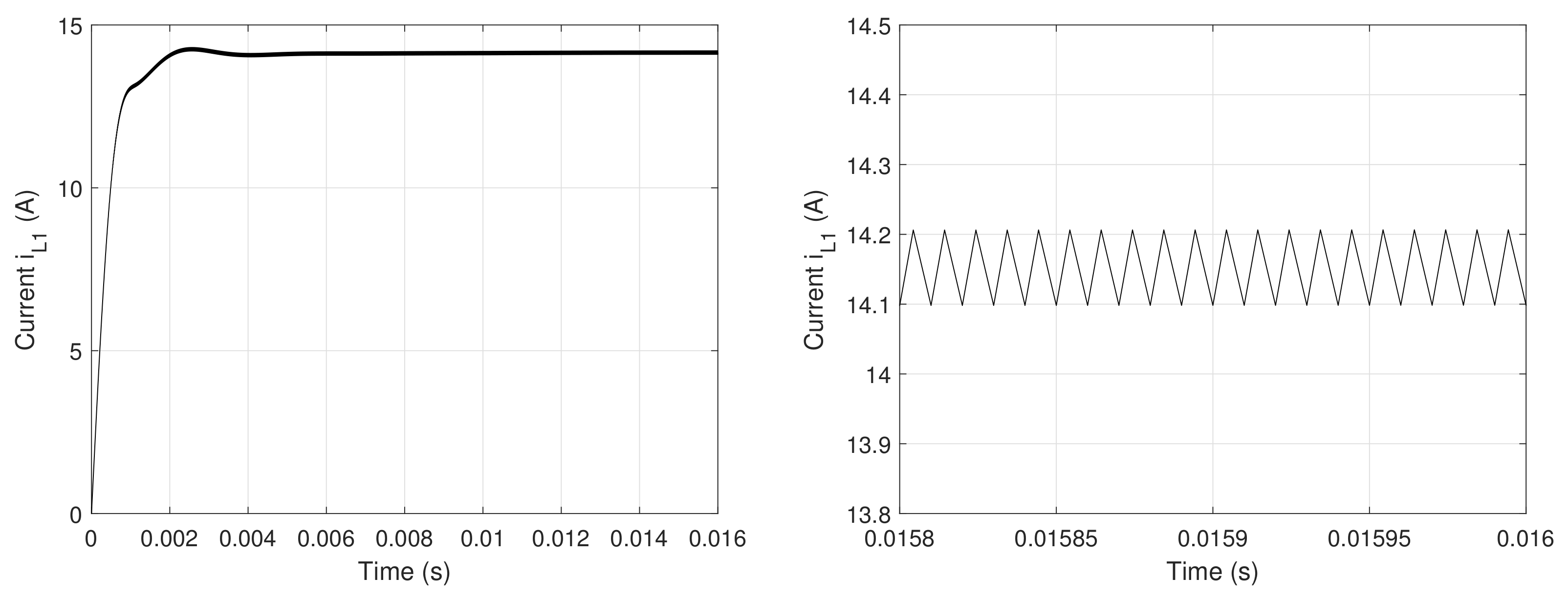
6.1. System Simulation under Healthy Conditions

The healthy conditions are considered when the $MO{S}_1$, $MO{S}_2$, and $MO{S}_3$ are fault-free, Equation, $h_1$ = $h_2$ = $h_3$ = 1. The stability can be deduced by the evaluation of the eigenvalues of the monodromy matrix ${\mathrm{\Phi }}_{cycle1}$ of Equation (28) as the load R changes from 1.5 $\mathrm{\Omega }$ to 2.5 $\mathrm{\Omega }$. This matrix has one complex conjugate pair and three real eigenvalues, illustrated in Figure 6.

Table 1. Eigenvalues of the monodromy matrix as R is varied in healthy switching case $h_1$ = $h_2$ = $h_3$ = 1.

R $\left(\mathbf{\Omega }\right)$	Real Eigenvalue 1	Real Eigenvalue 2	Real Eigenvalue 3	Complex Eigenvalues 45
$1.5$	$-0.97455$	$0.44760$	$0.99957$	$0.68191\pm i·1.24128$
$1.6$	$-0.93415$	$0.56232$	$0.99955$	$0.34386\pm i·1.14218$
$1.7$	$-0.9002$	$0.6547$	$0.99954$	$0.11025\pm i·1.04805$
2	$-0.82493$	$0.79446$	$0.99949$	$-0.24993\pm i·0.82523$
$2.2$	$-0.78907$	$0.83561$	$0.99947$	$-0.36023\pm i·0.71525$
$2.5$	$-0.74851$	$0.87052$	$0.99944$	$-0.44962\pm i·0.59171$

shows some values of the Floquet multipliers of the monodromy matrix ${\mathrm{\Phi }}_{cycle1}$ of Equation (28) under healthy conditions. One of the real values is close to unity. We observe in Figure 6 and Table 1 that the eigenvalues 4 and 5, for R = 1.5 $\mathrm{\Omega }$, are a pair of complex conjugated eigenvalues outside the unit circle, implying that the system is unstable. When R increases from 1.5 $\mathrm{\Omega }$ to 2.5 $\mathrm{\Omega }$, the eigenvalues 4 and 5 move outside of the unit circle and finally cross the unit circle towards each other. Crossing the unit circle, the system undergoes a bifurcation phenomenon, leading to the Neimark bifurcation. The inductor current $i_{L1}=x_2$ is plotted in the left and the right panels of Figure 7. Indeed, it can be observed that $x_2$ oscillates at the switching frequency $1/T$ = 100 kHz for R = 2.5 $\mathrm{\Omega }$. Decreasing R to 1.7 $\mathrm{\Omega }$, the chaotic behavior can also be observed.

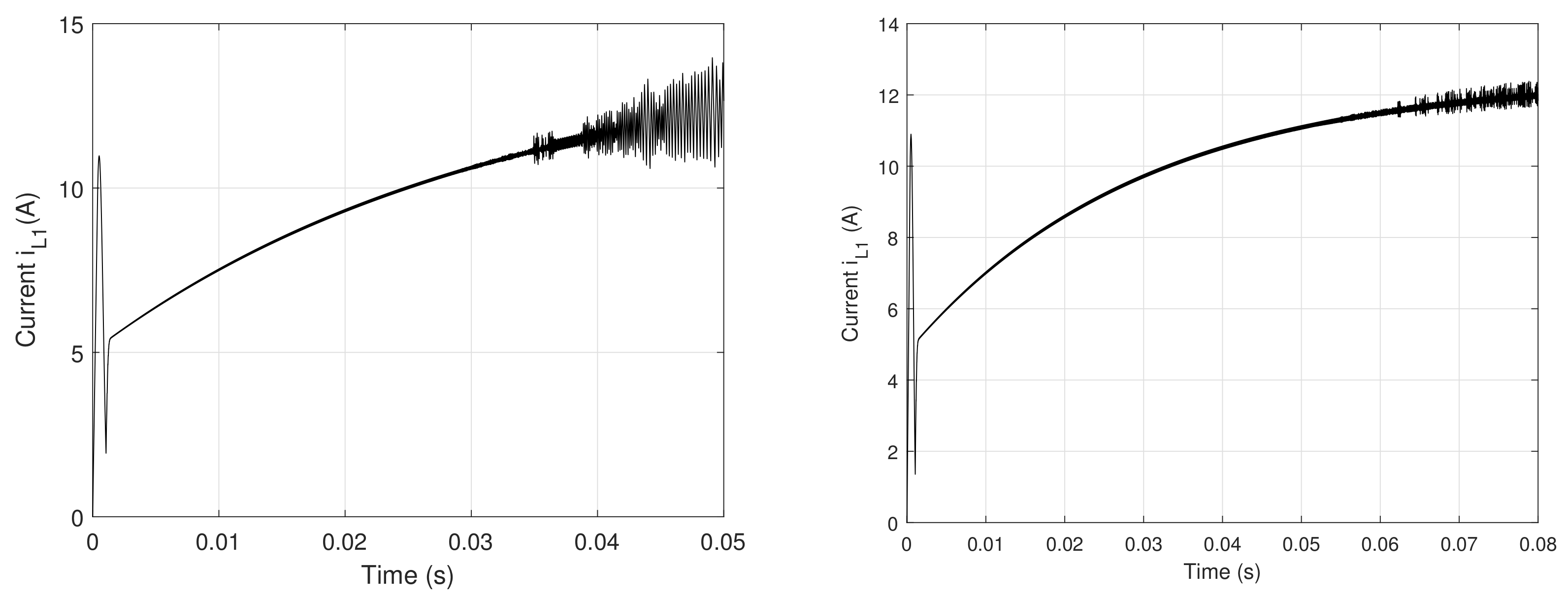
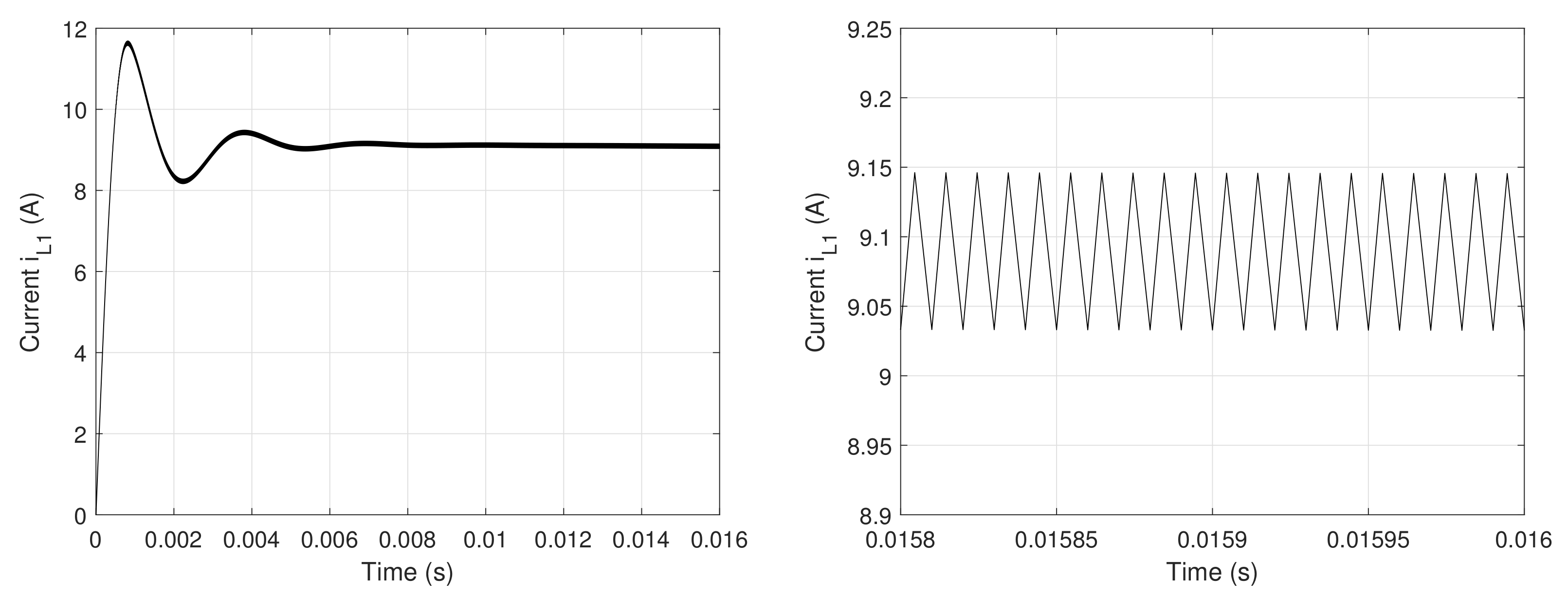
6.2. System Simulation under One Open-Circuit Faulty Condition

Let us consider that an open-circuit fault occurs in any $MOS$, e.g., in $MO{S}_3$ ($h_3$ = 0). The following can be extended to the two others, $MO{S}_1$ or $MO{S}_2$, considering the symmetry in the interleaved boost converter. The analysis is similar wherever the fault is located. A high current flows through the components immediately after the fault occurrence. A too-slow circuit protection could cause a failure: the currents $i_{L1}$, $i_{L2}$, $i_{L3}$ and the ripple of the output voltage $v_c$ are affected. The current $i_{L3}$ drops down to zero: this is why this state variable is outside of system analysis. Therefore, from now on, there are four state variables, $x_1$, $x_2$, $x_3$, and $x_4$: the capacitor voltage $v_c$, the inductor currents $i_{L1}$, $i_{L2}$, and the output of the integrator $v_i$. As a consequence, the subtraction of the current $i_{L3}$ (or using $h_3$ = 0) from the equations above, decreases the state vector from five to four elements. Inside the period T, there are four operation $modes$: $ON$ $OFF$, $ON$ $ON$, $OFF$ $ON$, and $OFF$ $OFF$, for the system under one open-circuit faulty condition. The evolution of the state variables in different $mode$ during $[0,T)$ can be described by four matrices $A_P$, $A_Q$, $A_R$, $A_S$ (4 × 4 dimension) by subtracting the fourth column and line of the Matrices (7) or (10), (13), (16) or (19), (22). The matrices $A_P$, $A_Q$, $A_R$, and $A_S$ can be defined as

$$A_P=\left[\begin{array}{cccc}-\frac{1}{RC}& \frac{{\overline{h}}_1}{C}& \frac{1}{C}& 0\\ \\ -\frac{{\overline{h}}_1}{L}& 0& 0& 0\\ \\ -\frac{1}{L}& 0& 0& 0\\ \\ -k_i{k}_c& 0& 0& 0\end{array}\right],A_Q=\left[\begin{array}{cccc}-\frac{1}{RC}& \frac{{\overline{h}}_1}{C}& \frac{{\overline{h}}_2}{C}& 0\\ \\ -\frac{{\overline{h}}_1}{L}& 0& 0& 0\\ \\ -\frac{{\overline{h}}_2}{L}& 0& 0& 0\\ \\ -k_i{k}_c& 0& 0& 0\end{array}\right],$$

(53)

and

$$A_R=\left[\begin{array}{cccc}-\frac{1}{RC}& \frac{1}{C}& \frac{{\overline{h}}_2}{C}& 0\\ \\ -\frac{1}{L}& 0& 0& 0\\ \\ -\frac{{\overline{h}}_2}{L}& 0& 0& 0\\ \\ -k_i{k}_c& 0& 0& 0\end{array}\right],A_S=\left[\begin{array}{cccc}-\frac{1}{RC}& \frac{1}{C}& \frac{1}{C}& 0\\ \\ -\frac{1}{L}& 0& 0& 0\\ \\ -\frac{{\overline{h}}_3}{L}& 0& 0& 0\\ \\ -k_i{k}_c& 0& 0& 0\end{array}\right].$$

(54)

In accordance with the diagram in Figure 8, the monotromy matrix

$${\mathrm{\Phi }}_{cycle2}=S_{SP}·{\mathrm{\Phi }}_S\left(T,\frac{T}{3}+dT\right)·S_{RS}·{\mathrm{\Phi }}_R\left(\frac{T}{3}+dT,\frac{T}{3}\right)·S_{QR}·{\mathrm{\Phi }}_Q\left(\frac{T}{3},dT\right)·S_{PQ}·{\mathrm{\Phi }}_P(dT,0),$$

(55)

has four exponential transition matrices and four saltation matrices. The transition matrices ${\mathrm{\Phi }}_P$, ${\mathrm{\Phi }}_Q$, ${\mathrm{\Phi }}_R$, and ${\mathrm{\Phi }}_S$ depend on the matrices $A_P$, $A_Q$, $A_R$, and $A_S$. The saltation matrices have the following form:

$$\begin{array}{c}\hfill S_{PQ}=\left[\begin{array}{cccc}1-\frac{(1-{\overline{h}}_2)·x_3{k}_p{k}_c}{de{n}_{PQ}·C}& -\frac{(1-{\overline{h}}_2)·x_3{k}_L}{de{n}_{PQ}·C}& 0& \frac{(1-{\overline{h}}_2)·x_3}{de{n}_{PQ}·C}\\ 0& 1& 0& 0\\ \frac{(1-{\overline{h}}_2)·x_1{k}_p{k}_c}{de{n}_{PQ}·L}& -\frac{(1-{\overline{h}}_2)·x_1{k}_L}{de{n}_{PQ}·L}& 1& -\frac{(1-{\overline{h}}_2)·x_1}{de{n}_{PQ}·L}\\ 0& 0& 0& 1\end{array}\right],\end{array}$$

(56)

with

$$de{n}_{PQ}=\left(k_i{k}_c-\frac{k_p{k}_c}{RC}-\frac{k_L{\overline{h}}_1}{L}\right)·x_1+k_p{k}_c\frac{{\overline{h}}_1}{C}·x_2+\frac{k_p{k}_c}{C}·x_3+\frac{k_L}{L}·V_{in}-k_i·V_{ref}.$$

(57)

and

$$\begin{array}{c}\hfill S_{RS}=\left[\begin{array}{cccc}1+\frac{(1-{\overline{h}}_2)·x_3{k}_p{k}_c}{de{n}_{RS}·C}& 0& \frac{(1-{\overline{h}}_2)·x_3{k}_L}{de{n}_{RS}·C}& -\frac{(1-{\overline{h}}_2)·x_3}{de{n}_{RS}·C}\\ 0& 1& 0& 0\\ -\frac{(1-{\overline{h}}_2)·x_1{k}_p{k}_c}{de{n}_{RS}·L}& 0& 1-\frac{(1-{\overline{h}}_2)·x_1{k}_L}{de{n}_{RS}·L}& \frac{(1-{\overline{h}}_2)·x_1}{de{n}_{RS}·L}\\ 0& 0& 0& 1\end{array}\right],\end{array}$$

(58)

with

$$de{n}_{RS}=\left(k_i{k}_c-\frac{k_p{k}_c}{RC}-\frac{k_L{\overline{h}}_2}{L}\right)·x_1+\frac{k_p{k}_c}{C}·x_2+k_p{k}_c\frac{{\overline{h}}_2}{C}·x_3+\frac{k_L}{L}·V_{in}-k_i·V_{ref}.$$

(59)

where $S_{SP}=S_{QR}={\mathbb{I}}_4$.

Once these matrices are found, the four eigenvalues of the monodromy matrix ${\mathrm{\Phi }}_{cycle2}$ (55) are determined (Figure 9), where the right panel is an extension of the left panel. Special attention is paid to the movement of the Floquet multipliers. Three eigenvalues remain inside of the unit circle and one is outside: they are given in

Table 2. Eigenvalues of the monodromy matrix in faulty switching case $h_3$ = 0, $h_1$ = $h_2$ = 1, as R varies.

R $\left(\mathbf{\Omega }\right)$	Real Eigenvalue 1	Real Eigenvalue 2	Real Eigenvalue 3	Real Eigenvalues 4
$1.5$	$0.862122$	$0.99999$	$0.999705$	$1.02199$
$1.6$	$0.056013$	$0.96466$	$0.999701$	$1.02531$
$1.7$	$0.079817$	$0.96455$	$0.999694$	$1.02867$
2	$0.166681$	$0.96329$	$0.999678$	$1.03943$
$2.2$	$0.234999$	$0.96187$	$0.999669$	$1.04763$
$2.5$	$0.349913$	$0.95898$	$0.999657$	$1.06275$

for some values of R. It can be observed that the fourth eigenvalue of the monodromy matrix ${\mathrm{\Phi }}_{cycle2}$ of Equation (55) is always superior to one, indicating a sudden loss of stability for any value of R inside the interval [1.5 $\mathrm{\Omega }$, 2.5 $\mathrm{\Omega }$].

When R increases from 1.5 $\mathrm{\Omega }$ to 2.5 $\mathrm{\Omega }$, the eigenvalues 4 are always outside of the unit circle: the system is unstable. Indeed, it can be observed that the inductor current $i_{L1}=x_2$ (plotted in the left panel of Figure 10 for R = 1.5 $\mathrm{\Omega }$) presents a no-periodicity undergoing to a chaotic behavior. It is essential to study the occurrence of chaos due to the variation of the system parameters. When a bifurcation occurs, an abrupt change in the steady-state behavior of the system also occurs. The very irregular form of $i_{L1}$ is due to the intrinsic nonlinear dynamics driven by the on and off durations of the switch $MOS$ which vary during a period of the clock. When R increases to 1.7 $\mathrm{\Omega }$, the behavior remains chaotic, as shown in the right panel of Figure 10. Figure 11 finally represents the inductor current $i_{L1}$ for R to 2.2 $\mathrm{\Omega }$. This periodic waveform is also called period – 2T, because the pattern of a large peak followed by a small peak is repeated approximately once every two clock cycles.

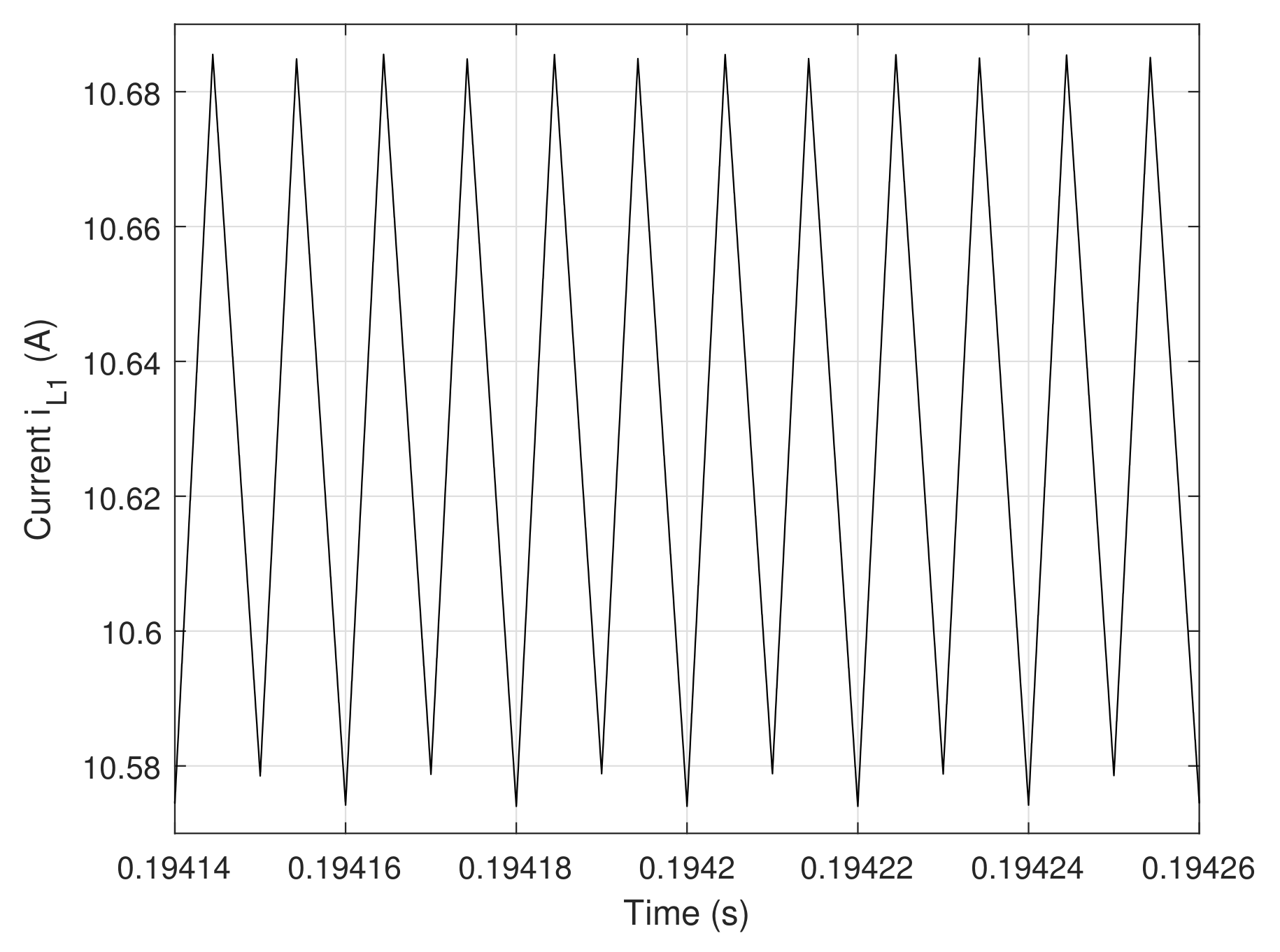
6.3. Development of a Fault-Tolerant Strategy with the Slope Compensation

The same voltage and inner current controller are employed for the closed loops control of the converter. Based on [26,27,35], it is possible to increase the stability with the movement of the eigenvalues from the outside to the inside of the unit circle, by changing the monodromy matrix ${\mathrm{\Phi }}_{cycle2}$ (55). The eigenvalues are outside of the unit circle in open-circuit faulty condition, which indicates instability. The monodromy ${\mathrm{\Phi }}_{cycle2}$ matrix depends on ${\mathrm{\Phi }}_P$, ${\mathrm{\Phi }}_Q$, ${\mathrm{\Phi }}_R$, and on ${\mathrm{\Phi }}_S$, and the saltation matrices $S_{PQ}$ and $S_{RS}$. The exponential of matrices ${\mathrm{\Phi }}_P$, ${\mathrm{\Phi }}_Q$, ${\mathrm{\Phi }}_R$, and ${\mathrm{\Phi }}_S$ depend on the state matrices $A_P$, $A_Q$, $A_R$, and $A_S$; they cannot be modified because they are dependent on the design of the converter [26,27]. To guarantee the stability of 1T-periodic orbit, we propose to modify the saltation matrices $S_{PQ}$ and $S_{RS}$ and, consequently, the switching functions. These switching functions affect the saltation matrices $S_{PQ}$ and $S_{RS}$ by their time derivatives. Changing the switching function by addition of a slope compensation, the time derivative of the saltation matrices can be influenced, in agreement with the observations reported in earlier studies [26,27]. The vector norm of the saltation matrices $S_{PQ}$ and $S_{RS}$ is independent of state values, because the control feedback is based on the change of the ramp time signal limits.

A fault-tolerant strategy with slope compensation is employed to avoid the instability illustrated in Figure 12. This strategy is applied to improve degraded mode operation and to allow continuity of functionality of the interleaved boost converter. The slope compensation requires few additional components (Figure 12) and has the following form:

$$V_{slope}=V_L+a·\frac{t}{T},$$

(60)

where $a=V_U-V_L$. Inside the interval [0,T) at $t=dT$ and $t=dT+T/3$, two switching conditions exist and have the following forms:

$$k_p{k}_c·x_1\left(dT\right)-k_p·V_{ref}-x_4\left(dT\right)-k_L·x_2\left(dT\right)+V_L+a·d=0,$$

(61)

and

$$k_p{k}_c·x_1(dT+T/3)-k_p·V_{ref}-x_4(dT+T/3)-k_L·x_3(dT+T/3)+\left(V_L+a·d+\frac{a}{3}\right)·e^{\frac{T}{3}}=0.$$

(62)

The elements of the saltation matrices $S_{PQ}$ and $S_{RS}$ have the following denominators:

$$de{n}_{PQ}=\left(k_i{k}_c-\frac{k_p{k}_c}{RC}-\frac{k_L{\overline{h}}_1}{L}\right)·x_1+k_p{k}_c\frac{{\overline{h}}_1}{C}·x_2+\frac{k_p{k}_c}{C}·x_3+\frac{k_L}{L}·V_{in}-k_i·V_{ref}+\frac{a}{T}.$$

(63)

$$de{n}_{RS}=\left(k_i{k}_c-\frac{k_p{k}_c}{RC}-\frac{k_L{\overline{h}}_2}{L}\right)·x_1+\frac{k_p{k}_c}{C}·x_2+k_p{k}_c\frac{{\overline{h}}_2}{C}·x_3+\frac{k_L}{L}·V_{in}-k_i·V_{ref}+\frac{a}{T}·e^{\frac{T}{3}}.$$

(64)

where $a/T$ and $(a/T)·e^{T/3}$ represent the time derivation of the surfaces.

Figure 13 shows the eigenvalues for several values of the load resistance R, indicating the stability of the interleaved boost converter. All the eigenvalues are inside the unit circle, as can be seen in

Table 3. Eigenvalues of the monodromy matrix in faulty switching case $h_1=h_2=1$, $h_3=0$ and with a slope compensation.

R $\left(\mathbf{\Omega }\right)$	Real Eigenvalue 1	Real Eigenvalue 2	Complex Eigenvalues 34
$1.5$	$0.984378$	$0.99999963$	$0.98864833\pm i·0.02452323$
$1.6$	$0.984235$	$0.99999962$	$0.98932429\pm i·0.02483646$
$1.7$	$0.984234$	$0.99999961$	$0.98992429\pm i·0.02509463$
2	$0.984229$	$0.99999959$	$0.99136832\pm i·0.02564743$
$2.2$	$0.984227$	$0.99999958$	$0.99211371\pm i·0.02589673$
$2.5$	$0.984225$	$0.99999957$	$0.99300967\pm i·0.02616516$

for certain values of R.

The inductor current $x_2=i_{L1}$ response with slope compensation for $R=1.5\mathrm{\Omega }$ and $R=2.5\mathrm{\Omega }$ is shown in Figure 14, respectively in Figure 15. It is clear that $x_2$ current, after a time transient (left panel of Figure 14, respectively left panel of Figure 15), settles down to the stable T-period limit cycle (right panel of Figure 14, respevtively right panel of Figure 15). A fault-tolerant strategy based on the slope compensation increases the stability of the interleaved boost converter under an open-circuit faulty condition within the whole range of the load R = 1.5–2.5 $\mathrm{\Omega }$. As its 1T-period orbit is stable, the eigenvalues of the monodromy matrix are all inside the unit circle.

7. Conclusions

Interleaved converters use an increasing number of power electronics switches; this is an opportunity to develop fault-tolerant strategies. We herein introduced a novel mathematical function enabling to simultaneously model both states (Equation, healthy and faulty conditions) of an MOS switch, leading to a unique model of the system. It is noticeable that the proposed function is universally applicable to any interleaved or single-phase dc–dc converter. Then, we focused on the converter stability under healthy or faulty conditions with the monodromy matrix and its Floquet multipliers. They indicate a partial stability of the system with healthy conditions (for an interval of the load values) due to a Neimark bifurcation, and a total instability in open-circuit faulty conditions. Then, we introduced a fault-tolerant strategy based upon the peak current control with slope compensation: not only does it extend the stable range of the load variation, but it also ensures stability in faulty conditions, on the same extended interval. Finally, the simulation results validate the effectiveness of our method and confirm the theoretical analysis with emphasis on the open-circuit fault-tolerance capability. In addition, the suggested fault strategy can be extended to other power stages used in different applications.

References

1. Aghdam, F.H.; Abapour, M. Reabilityand cost analysis of multistage boost converters connected to pv panels. IEEE J. Photovoltaics 2016, 6, 981–989. [Google Scholar] [CrossRef]
2. Ahmad, M.W.; Gorla, N.B.Y.; Malik, H.; Panda, S.K. A fault diagnosis and postfault reconguration scheme for interleaved boost converter in pv-based system. IEEE Trans. Power Electron 2021, 36, 3769–3780. [Google Scholar] [CrossRef]
3. Apablaza, D.; Munoz, J. Laboratory implementation of a boost interleaved converter for pv applications. IEEE Latin Am. 2016, 14, 2738–2743. [Google Scholar] [CrossRef]
4. Pei, T.; Hao, X. A fault detection method for photovoltaic systems based on voltage and current observation and evaluation. Energies 2019, 12, 1712. [Google Scholar] [CrossRef] [Green Version]
5. Guilbert, D.; N’Diaye, A.; Gaillard, A.; Djerdir, A. Fuel cell systems reliability and availability enhancement by developing a fast and efficient power switch open-circuit fault detection algorithm in interleaved dc-dc boost converter topologies. Int. J. Hydrogen Energy 2016, 41, 15505–15517. [Google Scholar] [CrossRef]
6. Seyezhai, R.; Mathur, B.L. A comparison of three-phase uncoupled and directly coupled interleaved boost converter for fuel cell applications. Int. J. Electr. Eng. Informatics 2011, 3, 394–407. [Google Scholar] [CrossRef]
7. Marcos-Pastor, M.; Vidal-Idiarte, E.; Cid-Pastor, A.; Martinez-Salamero, L. Interleaved digital power factor correction based on the sliding-mode approach. IEEE Trans. Power Electron. 2016, 31, 4641–4653. [Google Scholar] [CrossRef]
8. Garcia, O.; Zumel, P.; de Castro, A.; Cobos, A. Automotive dc-dc bidirectional converter made with many interleaved buck stages. SIAM Rev. 2008, 50, 578–586. [Google Scholar] [CrossRef]
9. Garcia, O.; Zumel, P.; de Castro, A.; Cobos, A. An automotive 16 phases dc-dc converter. In Proceedings of the 2004 IEEE 35th Annual Power Electronics Specialists Conference (IEEE Cat. No.04CH37551), Aachen, Germany, 20–25 June 2004; pp. 350–355. [Google Scholar]
10. Neugebauer, C.T.; Perreault, J. Computer aided optimisation of dc-dc converters for automotive applications. IEEE Trans. Power Electron. 2003, 18, 775–783. [Google Scholar] [CrossRef]
11. Banerjee, S.; Ghosh, A.; Rana, N. Design and fabrication of closed loop two-phase interleaved boost converter with type-iii controller. In Proceedings of the IECON—42th Annual Conference of the IEEE Industrial Electronics Society, Florence, Italy, 23–26 October 2016; Volume 14, pp. 3331–3336. [Google Scholar]
12. Hui, L.; Ke, M.; Poh, L.; Frede, H. Online fault identification based on an adaptive observer for modular multilevel converters applied to wind power generation systems. Energies 2015, 8, 7140–7160. [Google Scholar]
13. Ni, L.; Patterson, D.J.; Hudgins, J.L. Maximum power extraction from a small wind turbine using a 4-phase interleaved boost converter. In Proceedings of the IEEE Power Electronics and Machines in Wind Applications, Lincoln, NE, USA; 2009; Volume 11, pp. 1–5. [Google Scholar]
14. Givi, H.; Farjah, E.; Ghanbari, T. Switch and diode fault diagnosis in nonisolated dc-dc converters using diode voltage signature. Int. J. Circuit Theory Appl. 2018, 65, 1606–1615. [Google Scholar] [CrossRef]
15. Pei, X.; Nie, S.Y.; Chen, Y.; Kang, Y. Open-circuit fault diagnosis and fault-tolerant strategies for full-bridge dc-dc converters. IEEE Trans. Power Electron. 2012, 27, 2550–2565. [Google Scholar] [CrossRef]
16. Shahbazi, M.; Jamshidpour, E.; Poure, P.; Saadate, S.; Zolghadri, M.R. Open- and short-circuit switch fault diagnosis for non isolated dc-dc converters using field programmable gate array. IEEE Trans. Ind. Electron 2013, 60, 4136–4146. [Google Scholar] [CrossRef] [Green Version]
17. Shahbazi, M.; Zolghadri, M.R.; Ouni, S.; Zolghadri, M.R. Fast and simple open-circuit fault detection method for interleaved dc-dc converters. In Proceedings of the 7th PEDSTC, Tehran, Iran, 16–18 February 2016; pp. 440–445. [Google Scholar]
18. Wassinger, N.; Penovi, E.; Retegui, R.G.; Maestri, S. Open-circuit fault identification method for interleaved converters based on time-domain analysis of the state observer residual. IEEE Trans. Power Electron 2019, 34, 3740–3749. [Google Scholar] [CrossRef]
19. Wei, H.; Zhang, Y.; Yu, L.; Zhang, M. A new diagnostic algorithm for multiple igbts open circuit faults by the phase currents for power inverter in electric vehicles. Energies 2018, 11, 1508. [Google Scholar] [CrossRef] [Green Version]
20. Zhuo, S.; Xu, L.; Gaillard, A.; Huangfu, Y.; Gao, F. Robust open-circuit fault diagnosis of multi-phase interleaved dc-dc boost converter based on sliding mode observer. IEEE Trans. Transp. Electrif 2019, 5, 638–649. [Google Scholar] [CrossRef]
21. Bento, F.; Marques Cardoso, A.J. A comprehensive survey on fault diagnosis and fault tolerance of dc-dc converters. Chin. J. Electron. 2018, 12, 1–12. [Google Scholar]
22. Li, P.; Li, X.; Zeng, T. A fast and simple fault diagnosis method for interleaved dc-dc converters based on output voltage analysis. Electronics 2021, 10, 1451. [Google Scholar] [CrossRef]
23. Zhang, Z.; Zhou, H.; Deng, C.; Song, Q. Multiloop interleaved control for three-level buck converter in solar charging applications. IEICE Electron. Express 2018, 15, 20180369. [Google Scholar] [CrossRef] [Green Version]
24. Banerjee, S.; Verghese, G.C. Nonlinear Phenomena in Power Electronics: Attractors, Bifurcations, Chaos, and Nonlinear Control; IEEE Press: New York, NY, USA, 2001. [Google Scholar]
25. Tse, C.K. Complex Behavior of Switching Power Converters; CRC Press: New York, NY, USA, 2003. [Google Scholar]
26. Giaouris, D.; Banerjee, S.; Zahawi, B.; Pickert, V. Stability analysis of the continuous-conduction-mode Buck converter via Filippovs method. IEEE Trans. Circuits Syst. 2008, 55, 1084–1096. [Google Scholar] [CrossRef] [Green Version]
27. Giaouris, D.; Maity, S.; Banerjee, S.; Pickert, V.; Zahawi, B. Application of Filippov’s method for the analysis of subharmonic instability in dc-dc converters. Int. J. Circuit Theory Appl. 2009, 37, 899–919. [Google Scholar] [CrossRef] [Green Version]
28. Leine, R.I.; van Campen, D.H. Bifurcation phenomena in nonsmooth dynamical systems. Eur. J. Mech. Solids 2006, 25, 595–6168. [Google Scholar] [CrossRef]
29. Leine, R.I.; van Campen, D.H.; van de Vrande, B.L. Bifurcations in nonlinear discontinuous systems. Nonlinear Dyn. 2000, 23, 105–164. [Google Scholar] [CrossRef]
30. Morel, C.; Morel, J.-Y.; Petreus, D. Generalization of the Filippov method for systems with a large periodic input. Math. Comput. Simul. 2018, 146, 1–17. [Google Scholar] [CrossRef]
31. Di Bernardo, M.; Budd, C.J.; Champneys, A.R.; Kowalczyk, P.; Nordmark, A.B.; Tost, G.O.; Piiroinen, P.T. Bifurcations in nonsmooth dynamical systems. SIAM Rev. 2008, 50, 629–701. [Google Scholar] [CrossRef] [Green Version]
32. Kowalczyk, P.; di Bernardo, M. Two parameter degenerated sliding bifurcations in Filippov systems. Phys. D 2005, 20, 204–229. [Google Scholar] [CrossRef]
33. Kuznetsov, Y.A.; Rinaldi, S.; Gragnani, A. One-parameter bifurcations in planar Filippov systems. Int. J. Bifurc. Chaos 2003, 13, 2157–2188. [Google Scholar] [CrossRef] [Green Version]
34. Morel, C.; Petreus, D.; Rusu, A. Application of the Filippov method for the stability analysis of a photovoltaic system. Adv. Electr. Comput. Eng. 2011, 11, 93–98. [Google Scholar] [CrossRef]
35. Wu, H.; Pickert, V.; Giaouris, D.; Ji, B. Nonlinear analysis and control of interleaved boost converter using real-time cycle to cycle variable slope compensation. IEEE Trans. Power Electron. 2017, 32, 7256–7270. [Google Scholar] [CrossRef]
36. Ott, E.; Grebogi, C.; Yorke, J.A. Controlling chaos. Phys. Rev. Lett. 1990, 64, 1196. [Google Scholar] [CrossRef]
37. Goharrizi, A.Y.; Khaki-Sedigh, A.; Sepehri, N. Observer-based adaptative control of chaos in nonlinear discret-time systems using time-delayed state feedback. Chaos Solitons Fractal 2009, 41, 2448–2455. [Google Scholar] [CrossRef]
38. Wang, N.; Lu, G.N.; Peng, X.Z.; Cai, Y.K. A research on time delay feedback control performance in chaotic system of dc-dc inverter. In Proceedings of the 2013 IEEE International Conference on Vehicular Electronics and Safety, Dongguan, China, 28–30 July 2013; pp. 215–218. [Google Scholar]
Figure 1. Interleaved boost converter with V i n = 14 V, V r e f = 2.4 V, L 1 = L 2 = L 3 = L = 560 μ H, C = 300 μ F, R = 1.5 Ω –2.5 Ω , T = 0.00001 s, k i = 50, k c = 0.1, k p = 0.5, k L 1 = k L 2 = k L 3 = k L = 0.1.
Energies 15 00352 g001
Figure 2. Gate pulses of M O S 1 , M O S 2 , and M O S 3 , and the inductor currents i L 1 , i L 2 , and i L 3 in steady state.
Energies 15 00352 g002
Figure 3. One cycle of orbit evolution of state variables x ( t ) .
Energies 15 00352 g003
Figure 4. (a) Graph of the function f ( x ) ; (b) F ( x ) at t 0 goes over the instant t Σ with a smooth jump up to the instant T.
Energies 15 00352 g004
Figure 5. Diagram of the transition matrices and the saltation matrices in healthy switching case h 1 = h 2 = h 3 = 1.
Energies 15 00352 g005
Figure 6. Locus of the eigenvalues of the monodromy matrix with R variations under healthy conditions h 1 = h 2 = h 3 = 1.
Energies 15 00352 g006
Figure 7. Time-domain waveforms for different values of R (left panel R = 2.5 Ω , right panel R = 1.7 Ω ).
Energies 15 00352 g007
Figure 8. Diagram of the transition matrices and the saltation matrices in faulty switching case h 3 = 0, h 1 = h 2 = 1.
Energies 15 00352 g008
Figure 9. Locus of the eigenvalues of the monodromy matrix in faulty switching case h 3 = 0, h 1 = h 2 = 1, when R varies.
Energies 15 00352 g009
Figure 10. Time−domain waveforms for different values of R (left panel R = 1.5 Ω , right panel R = 1.7 Ω ) and in faulty switching case h 1 = h 2 = 1 , h 3 = 0 .
Energies 15 00352 g010
Figure 11. Time−domain waveform for R = 2 Ω in faulty switching case h 1 = h 2 = 1 , h 3 = 0 .
Energies 15 00352 g011
Figure 12. Interleaved boost converter with V i n = 14 V, V r e f = 2.4 V, L 1 = L 2 = L 3 = L = 560 μ H, C = 300 μ F, R = 1.5 Ω –2.5 Ω , T = 0.00001 s, k i = 50, k c = 0.1, k p = 0.5, k L 1 = k L 2 = k L 3 = k L = 0.1.
Energies 15 00352 g012
Figure 13. Locus of the eigenvalues of the monodromy matrix varying R in faulty switching condition h 1 = h 2 = 1 , h 3 = 0 , and with a slope compensation.
Energies 15 00352 g013
Figure 14. Time−domain waveforms for R = 1.5 Ω in faulty switching case h 1 = h 2 = 1 , h 3 = 0 , and with a slope compensation.
Energies 15 00352 g014
Figure 15. Time−domain waveforms for R = 2.5 Ω in faulty switching case h 1 = h 2 = 1 , h 3 = 0 , and with a slope compensation.
Energies 15 00352 g015