Sliding-Mode-Based Current and Speed Sensors Fault Diagnosis for Five-Phase PMSM

Abstract

The present paper deals with an active fault-tolerant speed tracking of a five-phase permanent magnet synchronous motor with currents and speed sensor failures. The active fault tolerant control scheme, integrating a sliding mode observer and backstepping controllers, is proposed to provide a continuous drive operation of the five-phase permanent magnet synchronous motor, even during more than one sensor fault occurrence. The sliding mode observer is designed to generate the residual signal necessary for the detection stage, whereas speed and current backstepping controllers handle the operation of the five-phase permanent magnet synchronous motor thanks to their ability to consider the nonlinearities of the system model in generating a control law that is robust enough in healthy and faulty cases. Furthermore, the FTC strategy uses the information received from the fault-tolerant switching block in terms of the measured and the observed currents and speed signals. To gain the maximum benefit of the sliding mode observer’s robustness to random noises and its ease of implementation, the observed currents and speed of the five-phase permanent magnet synchronous motor have been estimated. The simulation results are conducted to show the effectiveness of the proposed FTC control scheme and to prove its high performance in fault detection and tolerant control for the five-phase permanent magnet synchronous motor, since it significantly outperforms the performance provided by traditional methods.

1. Introduction

Nowadays, three-phase electrical machines powered by voltage inverters have demonstrated their efficiency at low powers. Nevertheless, at high powers, serious problems can arise, particularly in inverter switches that do not withstand the currents carried there. For these causes, increasing the number of phases in the motor drive is a well-founded solution to deliver the entire power between the different phases, thereby minimizing the stator current per phase and relieving the switches [1].

The most significant point, which is directly related to the present work, is the most obvious asset of multiphase machines, which is manifested in their excellent fault tolerance and enhanced acoustic behavior, realized by their lower torque ripples.

In the same context, the choice of the five-phase permanent magnet synchronous motor (5P-PMSM) can be justified for multiple industrial applications that require efficiency and reliability due to the restricted space available to lodge the electric and/or hybrid vehicle engine and its compactness [2]. Indeed, several fault types can arise in electrical devices. In the 5P-PMSM operating mode, some crucial faults related to sensor devices can occur. A primordial goal is to prevent external faults, such as sensor failures, from propagating into the actuator, which may generate hazard problem safety, production shutdown and various heavy industrial difficulties. These restrictions and/or conditions can be overcome by the fault-tolerant control (FTC) strategy based on compensating faults so as to prohibit fault events [3,4].

Nowadays, the 5P-PMSM has gained significant advantages in multiple FTC strategies, such as for EVs applications, power electrical drives, robotics and aerospace [5,6,7]. Indeed, the torque oscillations can be reduced by increasing the number of phases of the used system drive [8,9].

Several control methods for 5P-PMSMs have been investigated in the literature. The most widely used technique is the field-oriented control (FOC). It is well established and implemented in motor drive control systems. However, the FOC strategy is based on converting the 5P-PMSM to decoupled sub-machines in order to assimilate the electromagnetic torque to the DC motor dynamic.

However, the problems of nonlinearities in many complex systems are not considered. To address this problem, several nonlinear control approaches have been suggested, such as: the sliding mode control [10], the output linearization control [11], the fuzzy logic control [12] and the backstepping control [13].

In fact, for the most published research works, the backstepping control has been studied as a robust and efficient control strategy. In [14], it was proposed in sensorless control with a sliding mode observer. In [15], an adaptive backstepping control was developed for the entire asymptotic monitoring of motor speed and system variables based on a fuzzy logic controller. Herein, the backstepping control method for the speed and current control loops was developed for the 5P-PMSM control strategy.

The goal of the proposed technique was to mitigate the impact of unknown perturbations and the parameter change or variation on speed and currents to adjust nonlinear motor drive behavior.

The developed strategy demonstrated its ability to overcome the slope effect of the road and its ability to improve the tracking performance of the closed-loop system with variation in load torque. Indeed, the various failures that can affect the motor drive systems are related to speed and current sensors.

In fact, the motor drives can be affected by the converter’s faults (short-circuit or open-circuit semi-conductors) [16] and failures in various sensor types (mechanical or electrical) in the motor drive [17,18]. These faults cannot lead to a catastrophic incident if the safety level is very high. In [19], a new method has been proposed to detect the interturn short-circuit fault (ISCF) of a five-phase PMSM. The method first takes the command voltage and measured current of each phase winding as the original signal and then obtains the delay signal orthogonal to the original signal via Hilbert transform. A diagnosis of the open-phase fault of a five-phase permanent magnet synchronous motor was presented using harmonic current analysis [20]. The sensor fault has also been studied in [21], where the estimation and rejection strategy of current sensor faults for a PMSM drive system have been investigated. Sensor faults in current measurement circuits were treated as system disturbances by constructing a new system plant. However, the FTC structure proposed in [22] admits that, at minimum, two current sensors are necessary, and additional redundant transducers are applied. It has been proven that, after the current sensor fault occurs, its influence on the control structure, especially the speed transient, is compensated for by using non-sensitive components.

Several sensor faults for the electric system drive are interested in speed sensor faults. In [12], the main objective is the development and implementation of an FTC scheme for the speed control of a 5P-PMSM machine using a fuzzy logic controller (FLC). Some recent research studies have shown that the defective speed sensor is one of the most serious faults that can cause instability [23].

The current sensors can also be used for controlling system goals. To ensure an accurate operation mode, a machine drive has to be composed of at least four current sensors, a voltage sensor and a speed sensor. Inadequate measurements can affect the entire drive system. Sensors are exposed to several faults; for example, interruptions in a wire connection [24]. Especially abrupt harsh faults of a current sensor [25] result in the overcurrent dysfunction of the system, and if there is no relevant protection strategy in the gate-drive circuit, it leads to irremediable faults in the inverter. It is also important to note what the FTC scheme is based on using the current measurements; thus, a fault of a current sensor may lead to a wrong diagnosis, which can severely raise the repair time and cost.

Indeed, sensor faults, such as a bias in one of the five phase current sensors or speed sensors, can lead to the controller producing undesirable control actions, inducing serious consequences, such as important torque oscillations [26]. Recently, various fault diagnosis methods of current sensors have been presented. In [27], a Luenberger observer strategy based on an adaptive threshold to detect and isolate current sensor faults is presented. In [28], an average normalized currents approach to detect current sensor faults for PMSM drives is presented. In addition, the approach did not require any information about the machine model.

To mitigate the failure effects, diverse FTC schemes (active and passive) have been proposed in several research works. In [29], an FTC has been designed based on producing a variable residual signal so as to identify the internal system parameters change and an iterative adjustment methodology to optimize the obtained system achievement.

In [30], the FTC strategy for EV used a maximum-likelihood voting (MLV) technique that employs the speed sensor data and logical repetition. The Luenberger and the EKF observer have been approved for their capability to fulfill the EV entire speed variation for virtual sensors.

In [31], the hybrid active fault-tolerant control (AFTC) commutates between a traditional PI controller in the normal operating mode and a backstepping controller without a speed sensor to turn away any framework harm identified with the sensor issue occurring. With this control strategy, the estimation of the PMSG rotor position was ensured by a sliding mode observer.

In the literature, it has been affirmed that the precision in location and analysis of sensor shortcomings in the electrical motor drive frameworks is the fundamental advancement for the FTC technique. This stage relies on the influence of observation errors.

In fact, various observers in the FTC scheme have been suggested; among them, the sliding mode observer seems to be a good alternative, as it proves their accuracy in estimation even in a harsh and stochastic environment [32]. For this reason, this method finds a great research interest in sensorless control.

It is important to mention that multiple research studies investigating FTC strategies are based on three-phase PMSM using classical PI controllers for speed and current loops [33]. In [34], a fault-tolerant control structure for the Induction Motor (IM) drive has been described and the influence of current sensor faults on the properties of the vector-controlled IM drive system was analyzed. In the proposed approach, the information about the stator currents components is required. To achieve this, the possibility of the neural network application in detecting stator current sensor faults in the vector control algorithm is introduced and discussed.

In the same context, a Fault Tolerant (FT) vector-controlled induction motor drive system has been described in [35] and has been tested under various drive conditions. The influence of the rotor speed sensor faults on the properties of the analyzed drive has been tested. Faults detection technics based on different algorithms were developed and described. The simulation and experimental results prove the efficiency of the FT method.

Otherwise, the fault-tolerant Direct Field Oriented Control (DFOC) of an induction motor drive has been studied in [36]. Particularly, the influence of the stator current sensor faults on the properties of the DFOC drive system has been presented. The simple algorithmic/logical mechanism, based on the measured currents, was used for the current sensor fault detection. For the calculation of the stator current components (in the stationary reference frame), other algebraic relations based on the signals from the active sensors were used.

The choice of 5P-PMSM is very attractive because this machine type can work in faulty conditions, such as the opening phase. In addition, PI controllers were developed for motor drive systems with mathematical models that are facilitated by using simplifying hypotheses. However, in the case of the occurrence of an external perturbation, unmodeled uncertainties or a fault, then these regulators are inadequate to correctly (reasonably) monitor the motor drive.

In fact, the use of a backstepping technique in the suggested FTC scheme using a sliding mode observer has been proposed to ensure a significant performance concerning precision and stability, even when the studied system includes an important complexity and/or nonlinearity.

The aim of the paper is to present an easy and efficient active FTC scheme applied to 5P-PMSM. The FTC strategy proposed here is convenient for detecting exactly the current and the speed sensor faults and provides, for these signals, information about the detected fault. Its other competitive asset is that only the accessible input/output measurements are needed in the system without additional hardware data. It also uses both the robust backstepping controllers for speed and current loops and the Sliding Mode Observer (SMO) to estimate these signals. The speed and current loops only use the measured signals supplied by the corresponding sensors for a nominal model without perturbations.

Nevertheless, during external perturbations or fault occurrence, the switching fault tolerant block is activated and the FTC algorithm allows for a calculation of the reconstructed signals used after the system feedback.

This configuration strategy enhances the system reliability and ensures the security of the 5P-PMSM through the efficient detection of speed and current sensors.

This research work is structured as follows: Section 2 presents the 5P-PMSM model description. Section 3 introduces the rotor speed backstepping controller to monitor the 5P-PMSM speed. In Section 4, the backstepping current controllers are developed to guarantee a disturbance compensation. The SMO is employed for the speed and currents estimation required in the proposed fault tolerant algorithm. To reduce the fault effect, a FTC strategy using backstepping/SMO techniques is presented in Section 6 and the simulation numerical tests are illustrated to prove its efficiency. Finally, Section 7 concludes the work and suggests future perspectives.

2. Modeling of 5P-PMSM

2.1. 5P-PMSM Model in Natural Frame

The equation of the stator voltage of the 5P-PMSM in the natural frame can be expressed as follows:

$$V_s=R_s·i_{sk}+\frac{d{\mathsf{\Phi }}_{sk}}{dt}+e_{sk}$$

(1)

where $k=1,2,3,4,5$ is the number of the phase, ${\mathsf{\Phi }}_{sk}$ is the stator flux in the $k^{th}$ phase, $e_{sk}$ is the EMF produced by the permanent magnet in the $k^{th}$ stator phase and $R_s$ is the stator resistance, which is the same for all of the five phases. The EMF can be expressed by:

$$e_{sk}=f_k\left(\theta \right){\omega }_m$$

(2)

Considering regularly shifted phases and overlooking the saturation and salience effects, the stator flux expression is described as:

$$\left[\begin{array}{c}{\mathsf{\Phi }}_{s1}\\ {\mathsf{\Phi }}_{s2}\\ {\mathsf{\Phi }}_{s3}\\ {\mathsf{\Phi }}_{s4}\\ {\mathsf{\Phi }}_{s5}\end{array}\right]=\left[\begin{array}{ccccc}L& M_{s1}& M_{s2}& M_{s2}& M_{s1}\\ M_{s1}& L& M_{s1}& M_{s2}& M_{s2}\\ M_{s2}& M_{s1}& L& M_{s1}& M_{s2}\\ M_{s2}& M_{s2}& M_{s1}& L& M_{s1}\\ M_{s1}& M_{s2}& M_{s2}& M_{s1}& L\end{array}\right]\left[\begin{array}{c}\begin{array}{c}{i}_{s1}\\ i_{s2}\\ i_{s3}\end{array}\\ i_{s4}\\ i_{s5}\end{array}\right]$$

(3)

where L is the proper inductance, also called the self-inductance of a phase, and M_s1 and M_s2 are the mutual inductance between two phases shifted, respectively, by 2π/5 and 4π/5. This vector representation simplifies the calculation of the electromagnetic torque, and the different power of the machine, such as the instantaneous power of the 5P-PMSM, which can be obtained as follows:

$$P={\displaystyle \sum }_{k=1}^5{V}_{sk}{i}_{sk}$$

(4)

Using (1), the 5P-PMSM power can be written as follows:

$$P={\displaystyle \sum }_{k=1}^5\left(\underset{P_1}{\underbrace{R{i}_{sk}^2}}+\underset{P_2}{\underbrace{\frac{d\theta }{dt}{i}_{sk}}}+\underset{P_3}{\underbrace{e_{sk}{i}_{sk}}}\right)$$

(5)

where $P_1$, $P_2$ and $P_3$ are, respectively, the Joule losses, the magnetic power and the electromechanical power. P₃ represents the electromagnetic torque, which is a product of EMFs and currents:

$$T_{em}=\frac{1}{{\omega }_m}\left(e_{s1}{i}_{s1}+e_{s2}{i}_{s2}+e_{s3}{i}_{s3}+e_{s4}{i}_{s4}+e_{s5}{i}_{s5}\right)$$

(6)

The EMF in the natural frame can be expressed by the following equation:

$$e_{sk}={\displaystyle \sum }_{h=1}^{\infty }{E}_{h}sin\left(h\left(n_p\theta -(k-1\right)\frac{2\pi }{5}\right)$$

(7)

For the 5P-PMSM, only the fundamental and the third-order harmonic components are employed in the EMF expression in every phase:

$$\left[\begin{array}{c}{e}_{s1}\\ e_{s2}\\ e_{s3}\\ e_{s4}\\ e_{s5}\end{array}\right]=-{\Lambda }_1·\left[\begin{array}{c}\sin ({\theta }_r)\\ \sin ({\theta }_r-\frac{2\pi }{5})\\ \sin ({\theta }_r-\frac{4\pi }{5})\\ \sin ({\theta }_r-\frac{6\pi }{5})\\ \sin ({\theta }_r-\frac{8\pi }{5})\end{array}\right]-3·{\Lambda }_3·\left[\begin{array}{c}\sin (3{\theta }_r)\\ \sin 3\left({\theta }_r-\frac{2\pi }{5}\right)\\ \sin 3\left({\theta }_r-\frac{4\pi }{5}\right)\\ \sin 3\left({\theta }_r-\frac{6\pi }{5}\right)\\ \sin 3\left({\theta }_r-\frac{8\pi }{5}\right)\end{array}\right]$$

(8)

where: ${\Lambda }_1={\varphi }_{f1}{\omega }_m$; ${\Lambda }_3={\varphi }_{f3}{\omega }_m$.

2.2. 5P-PMSM Model in Rotating Fram

For controlling machine drives, several transformations are applied in order to simplify the 5P-PMSM model. For this reason, an arbitrary transformation matrix is used for changing the 5P-PMSM variables to the reference frame rotating at the synchronous angular velocity [37]. The rotating frame is divided into primary (d_p-q_p) and secondary (d_s-q_s) coordinates when the (d_s-q_s) one is rotating at three times the synchronous velocity. Indeed, this transformation is divided into two matrices: Clark (a-b-c-d-e to α_p-β_p-α_s-β_s) and Park (α_p-β_p-α_s-β_s to d_p-q_p-d_s-q_s) transformations. Then:

$${\vartheta }^{\left(d_p{q}_p{d}_s{q}_s\right)}={T\vartheta }^{\left(abcde\right)}=T_{Park}{T}_{Clark}\vartheta {}^{\left(abcde\right)}$$

(9)

where:

$$T=T_{Park}{T}_{Clark}; {\mathsf{\vartheta }}^{\left(abcde\right)}={\left[{\mathsf{\vartheta }}_a{\mathsf{\vartheta }}_b{\mathsf{\vartheta }}_c{\mathsf{\vartheta }}_d{\mathsf{\vartheta }}_e\right]}^T; \mathrm{and} {\mathsf{\vartheta }}^{\left(d_p{q}_p{d}_s{q}_s\right)}={\left[{\mathsf{\vartheta }}_{dp }{\mathsf{\vartheta }}_{qp}{\mathsf{\vartheta }}_{ds}{\mathsf{\vartheta }}_{qs}\right]}^T.$$

Applying these transformations, the obtained model in the (d,q) frame can be presented by the following system equations:

$$\{\begin{array}{c}{V}_d^p=R{i}_d^p+L_p\frac{d{i}_d^p}{dt}-n_p {\omega }_m{L}_p{i}_q^p\\ V_q^p=R{i}_q^p+L_p\frac{d{i}_q^p}{dt}+n_p {\omega }_m{L}_p{i}_d^p+\sqrt{\frac{5}{2}} n_p{\varphi }_{f1}{\omega }_m\\ V_d^s=R{i}_d^s+L_s\frac{d{i}_d^s}{dt}-3 n_p{\omega }_m L_s{i}_q^s\\ V_q^s=R{i}_q^s+L_s\frac{d{i}_q^s}{dt}+3 n_p {\omega }_m L_s{i}_d^s+\sqrt{\frac{5}{2}} n_p{\varphi }_{f3}{\omega }_m\\ T_{em}=\sqrt{\frac{5}{2}}·n_p·\left({\varphi }_{f1}{i}_q^p+{\varphi }_{f3}{i}_q^s\right)\end{array}$$

(10)

where $V_d^p$, $V_q^p$, $V_d^s$ and $V_q^s$ are the stator voltages in the $d_p$, $q_p$, $d_s$ and $q_s$ axis, respectively, and $i_d^p$, $i_q^p$, $i_d^s$ and $i_q^s$ are the stator currents in the $d_p$, $q_p$, $d_s$ and $q_s$ axis, respectively.

The electromagnetic torque equation $T_{em}$ given in (10), demonstrates that the third current harmonic component contributes in the generation of the motor torque [38].

The mechanical equation is given by:

$$J\frac{d{\omega }_m}{dt}=T_{em}-f{\omega }_m-T_L$$

(11)

where $T_{em}$, ${\omega }_m$, f and J are the developed electromagnetic torque, the motor speed, the friction coefficient and the inertia of the electric driving motor, respectively.

In fact, the 5P-PMSM model complexity, which leads to a large number of coupled equations, can be averted by using the (d_p,q_p) reference frame for the fundamental components and the (d_s,q_s) reference frame for the third harmonic components.

Using (10), the equivalent 5P-PMSM model can be rewritten as follows:

$$\{\begin{array}{c}\frac{d{i}_d^p}{dt}=\frac{1}{L_p}·V_d^p+h_1\\ \frac{d{i}_q^p}{dt}=\frac{1}{L_p}·V_q^p+h_2\\ \begin{array}{c}\frac{d{i}_d^s}{dt}=\frac{1}{L_s}·V_d^s+h_3\\ \frac{d{i}_q^s}{dt}=\frac{1}{L_s}·V_q^s+h_4\\ \frac{d{\omega }_m}{dt}=h_5\end{array}\end{array}$$

(12)

With:

$$\begin{array}{c}{h}_1=-\frac{R}{L_p}{i}_d^p+n_p·{\omega }_m·i_d^p\\ h_2=-\frac{R}{L_p}{i}_q^p-n_p·{\omega }_m·i_q^p-\frac{1}{L_p}\sqrt{\frac{5}{2}}·n_p·{\varphi }_{f1}·{\omega }_m\\ h_3=-\frac{R}{L_s}{i}_d^s+3·n_p·{\omega }_m·i_d^s\\ h_4=-\frac{R}{L_s}{i}_q^s-3·n_p·{\omega }_m·i_q^s-\frac{1}{L_s}\sqrt{\frac{5}{2}}·n_p·{\varphi }_{f3}{\omega }_m\\ h_5=\frac{1}{J}\left(T_{em}-B·{\omega }_m-T_L\right)=\frac{1}{J}\left(\sqrt{\frac{5}{2}}·n_p·\left({\varphi }_{f1}{i}_q^p+{\varphi }_{f3}{i}_q^s\right)-B·{\omega }_m-T_L\right)\end{array}$$

(13)

In the electric motor drives’ feedback, the classical PI controllers are usually applied in the speed and currents loops, although their use becomes limited in front of the machine model variation.

In the feedback of electric motor drives, classical PI controllers are commonly used in speed and currents loops, whereas their use is restricted in front of the machine model variation. This variation can be caused by the parametric fluctuation or failure occurrence, such as abrupt power supply opening phases.

Therefore, it is necessary to use a control law that is insensitive to external perturbations and that can withstand the non-linearity of the system to be controlled, in order to overcome such problems.

In this research work, the backstepping control procedure is selected to achieve the above control requirements.

2.3. Power Converter

The five-phase motor was fed by a five-leg VSI inverter. The modulation algorithm used is the conventional PWM technique. The topology of the used inverter is described in Figure 1. Therefore, the switching states result from the application of this technique. The voltages at the 5P-PMSM terminals are obtained from the switching states of each leg based on the Relation (14), where Si = 1 if the upper switch is on and Si = 0 for the opposite case.

$$\left[\begin{array}{c}{\nu }_{as}\\ {\nu }_{bs}\\ {\nu }_{cs}\\ {\nu }_{ds}\\ {\nu }_{es}\end{array}\right]=\left[\begin{array}{ccccc}4& -1& -1& -1& -1\\ -1& 4& -1& -1& -1\\ -1& -1& 4& -1& -1\\ -1& -1& -1& 4& -1\\ -1& -1& -1& -1& 4\end{array}\right] \left[\begin{array}{c}{\nu }_{as}\\ {\nu }_{bs}\\ {\nu }_{cs}\\ {\nu }_{ds}\\ {\nu }_{es}\end{array}\right]$$

(14)

3. Speed Backstepping Control Design

The key idea of the backtracking approach is to convert a completely complicated closed-loop system into an equivalent sequence cascaded into lower-order subsystems and then to develop an intermediate control law based on the Lyapunov function to take advantage of the stress on robustness, the global asymptotic stability and the better system transient performance control.

In fact, the method consists of successive process stages; a virtual intermediate control signal is generated at each step to ensure the convergence of the system to a steady-state.

This can be achieved using Lyapunov functions, which ensure a step-by-step stabilization of every synthesis step [39]. Herein, the goal of applying this control is to allow for the 5P-PMSM speed to more precisely track the corresponding reference speed while keeping the current i_dp equal to zero.

The backstepping synthesis controller requires various system information. This implies the implementation of multiple sensors, such as currents, voltages and speed/position sensors. Indeed, these sensors are delicate to external conditions and increase the system expense. In order to surmount such drawbacks, the SMO observer is used in this work. This choice is based on its ability to estimate the different system states, and to ensure a high reliability in case of an occurring sensor fault.

The motor speed tracking error is given by the following equation:

$$e_{{\omega }_m}={\omega }_m^{*}-{\widehat{\omega }}_m$$

(15)

Here, ${\omega }_m^{*}$ is the reference speed and ${\widehat{\omega }}_m$ is the estimated speed obtained from the SMO. The error variation is given by (16) as follows:

$${\dot{e}}_{{\omega }_m}={\dot{\omega }}_m^{*}-\dot{{\widehat{\omega }}_m}$$

(16)

Considering Equations (12) and (16), the previous relation can be described as follows:

$${\dot{e}}_{{\omega }_m}={\dot{\omega }}_m^{*}-{\widehat{h}}_5$$

(17)

where:

$${\widehat{h}}_5=\frac{1}{J}\left({\widehat{T}}_{em}-B·{\widehat{\omega }}_m-T_L\right)$$

(18)

To verify the tracking performance, the first function of Lyapunov $V_1$ is chosen as follows:

$$V_1=\frac{1}{2}{e}_{{\omega }_m}^2$$

(19)

Using Equation (17), the derivative of (19) is given by:

$${\dot{V}}_1=e_{{\omega }_m}{\dot{e}}_{{\omega }_m}=e_{{\omega }_m}\left({\dot{\omega }}_m^{*}-{\widehat{h}}_5\right)$$

(20)

Using Equations (10) and (20), this derivative becomes as follows:

$${\dot{V}}_1=e_{{\omega }_m}\left({\dot{\omega }}_m^{*}-\frac{1}{J}\left({\widehat{T}}_{em}-B {\widehat{\omega }}_m-T_L\right)\right)$$

(21)

To fulfill the Lyapunov stability criteria, Equation (21) can be expressed as follows:

$${\dot{V}}_1=-k e_{{\omega }_m}^2+e_{{\omega }_m}\left(\lambda e_{{\omega }_m}+{\dot{\omega }}_m^{*}-\frac{1}{J}\left({\widehat{T}}_{em}-B {\widehat{\omega }}_m-T_L\right)\right)$$

(22)

The local asymptotic stability of the speed and current closed loops is attained, except that the Lyapunov condition ${\dot{V}}_1<0$ is verified and validated; this imposes the following restriction:

$$\{\begin{array}{c}\lambda e_{{\omega }_m}+{\dot{\omega }}_m^{*}-\frac{1}{J}\left({\widehat{T}}_{em}-B {\widehat{\omega }}_m-T_L\right)=0\\ \lambda >0\end{array}$$

(23)

The derivative of the Lyapunov function is finally obtained in the following form:

$${\dot{V}}_1=-\lambda e_{{\omega }_m}^2$$

(24)

Using Equation (23), the desired electromagnetic torque $T_e^{*}$, which produces the stabilizing functions, can be obtained as follows:

$$T_e^{*}=J\left(\lambda e_{{\omega }_m}+{\dot{\omega }}_m^{*}+\frac{B}{J} {\widehat{\omega }}_m+\frac{1}{J}{T}_L\right)$$

(25)

where ${\widehat{\omega }}_m$ is the estimated rotor speed and the output of the SMO, which replaces the measured sensor value during the failure event; hence, in the healthy operation mode, the sensor value sensor will be used instead.

Using Equation (25), the reference current components $i_q^{p*}$ can be determined as follows:

$$i_q^{p*}=\left(\lambda e_{{\omega }_m}+{\dot{\omega }}_m^{*}+\frac{B}{J}{\widehat{\omega }}_m+\frac{1}{J}{\widehat{T}}_L\right)/a$$

(26)

where $i_q^{p*}$ is the reference current value produced by the backstepping speed controller, which is the image of the electromagnetic torque.

With:

$$a=\left(\sqrt{\frac{5}{2}}{n}_p{\varphi }_{f1}\right)/J \mathrm{and} \{\begin{array}{c}{i}_d^{p*}=0\\ i_d^{s*}=0\\ i_q^{s*}=0\end{array}$$

(27)

The speed and current backstepping controllers will receive the required input signals from the FTC blocks. The comparison between the measured and the estimated speed and current values is exploited in generating the errors, which are then compared with the threshold to produce the fault indicator. In this paper, we propose developing the backstepping current controllers instead of the classical PI ones.

4. Currents Backstepping Control

In this section, the goal is to establish the reference currents calculated previously. The errors of the following currents are defined as follows:

$$\{\begin{array}{c}\begin{array}{c}{e}_{idp}=i_d^{p*}-i_d^p\\ e_{iqp}=i_q^{p*}-i_q^p\\ e_{ids}=i_d^{s*}-i_d^s\end{array}\\ e_{iqs}=i_q^{s*}-i_q^s\end{array}$$

(28)

The derivative of the current error is then expressed by (29):

$$\{\begin{array}{c}\begin{array}{c}{\dot{e}}_{idp}={\dot{i}}_d^{p*}-{\dot{i}}_d^p\\ {\dot{e}}_{iqp}={\dot{i}}_q^{p*}-{\dot{i}}_q^p\\ {\dot{e}}_{ids}={\dot{i}}_d^{s*}-{\dot{i}}_d^s\end{array}\\ {\dot{e}}_{iqs}={\dot{i}}_q^{s*}-{\dot{i}}_q^s\end{array}$$

(29)

Using the current dynamics in (12), Equation (29) can be written as follows:

$$\{\begin{array}{c}\begin{array}{c}{\dot{\mathit{e}}}_{\mathit{i}\mathit{d}\mathit{p}}={\mathit{i}}_{\mathit{d}}^{\mathit{p}\ast }-\frac{\mathbf{1}}{{\mathit{L}}_{\mathit{p}}}{\mathit{v}}_{\mathit{d}}^{\mathit{p}}-{\mathit{h}}_{\mathbf{1}}\\ {\dot{\mathit{e}}}_{\mathit{i}\mathit{q}\mathit{p}}={\mathit{i}}_{\mathit{q}}^{\mathit{p}\ast }-\frac{\mathbf{1}}{{\mathit{L}}_{\mathit{p}}}{\mathit{v}}_{\mathit{q}}^{\mathit{p}}-{\mathit{h}}_{\mathbf{2}}\\ {\dot{\mathit{e}}}_{\mathit{i}\mathit{d}\mathit{s}}={\mathit{i}}_{\mathit{d}}^{\mathit{s}\ast }-\frac{\mathbf{1}}{{\mathit{L}}_{\mathit{s}}}{\mathit{v}}_{\mathit{d}}^{\mathit{s}}-{\mathit{h}}_{\mathbf{3}}\end{array}\\ {\dot{\mathit{e}}}_{\mathit{i}\mathit{q}\mathit{s}}={\mathit{i}}_{\mathit{q}}^{\mathit{s}\ast }-\frac{\mathbf{1}}{{\mathit{L}}_{\mathit{s}}}{\mathit{v}}_{\mathit{q}}^{\mathit{s}}-{\mathit{h}}_{\mathbf{4}}\end{array}$$

(30)

According to (21), h₅ and the dynamics of the reference speed can be expressed in the following forms:

$${\widehat{h}}_5=\frac{1}{J}\left({\widehat{T}}_{em}-B {\widehat{\omega }}_m-T_L\right)=\frac{1}{J}\left(\sqrt{\frac{5}{2}} n_p·\left({\varphi }_{f1}{i}_q^p+{\varphi }_{f3}{i}_q^s\right)-B{\widehat{\omega }}_m-T_L\right)$$

(31)

Using (30), the reference speed derivative is:

$${\dot{\omega }}_m^{*}=\frac{1}{J}\left(\sqrt{\frac{5}{2}} n_p\left({\varphi }_{f1}{i}_q^p+{\varphi }_{f3}{i}_q^s\right)-B {\widehat{\omega }}_m-T_L\right)-\lambda e_{{\omega }_m}$$

(32)

Using (30), Equation (32) can be expressed as follows:

$${\dot{\omega }}_m^{*}=\frac{1}{J}\left(\sqrt{\frac{5}{2}} n_p\left({\varphi }_{f1}{e}_{iqp}+{\varphi }_{f3}{e}_{iqs}\right)\right)-\lambda e_{{\omega }_m}+{\widehat{h}}_5\mathrm{b}$$

(33)

Then, the dynamics of the velocity error represented by Equation (17) is written as:

$$\dot{{\mathit{e}}_{{\mathit{\omega }}_{\mathit{m}}}}=\frac{\mathbf{1}}{\mathit{J}}\left(\sqrt{\frac{\mathbf{5}}{\mathbf{2}}} {\mathit{n}}_{\mathit{p}}\left({\varphi }_{\mathit{f}\mathbf{1}}{\mathit{e}}_{\mathit{i}\mathit{q}\mathit{p}}+{\varphi }_{\mathit{f}\mathbf{3}}{\mathit{e}}_{\mathit{i}\mathit{q}\mathit{s}}\right)\right)-\lambda {\mathit{e}}_{{\mathit{\omega }}_{\mathit{m}}}$$

(34)

It is notable that the Equation system (30) includes the expression of the 5P-PMSM stator voltages. This allows us to establish a new Lyapunov function based on stator current errors and the speed error:

$${\mathit{V}}_{\mathbf{2}}=\frac{{\mathit{e}}_{\mathit{\omega }\mathit{m}}^{\mathbf{2}}+{\mathit{e}}_{\mathit{i}\mathit{d}\mathit{p}}^{\mathbf{2}}+{\mathit{e}}_{\mathit{i}\mathit{q}\mathit{p}}^{\mathbf{2}}+{\mathit{e}}_{\mathit{i}\mathit{d}\mathit{s}}^{\mathbf{2}}+{\mathit{e}}_{\mathit{i}\mathit{q}\mathit{s}}^{\mathbf{2}}}{\mathbf{2}}$$

(35)

The Lyapunov’s function derivative (36) is given by:

$${\dot{V}}_2=e_{\omega m}{\dot{e}}_{\omega m}+e_{idp}{\dot{e}}_{idp}+e_{iqp}{\dot{e}}_{iqp}+e_{ids}{\dot{e}}_{ids}+e_{iqs}{\dot{e}}_{iqs}$$

(36)

By substituting (30) and (34) in (36), we can obtain:

$$\begin{array}{c}{\dot{V}}_2=-\lambda e_{\omega e}^2-{\lambda }_1{e}_{idp}^2-{\lambda }_2{e}_{iqp}^2-{\lambda }_3{e}_{ids}^2-{\lambda }_4{e}_{iqs}^2\hfill \\ +e_{idp}\left({\lambda }_1{e}_{idp}+{\dot{i}}_d^{\ast p}-\frac{1}{L_p}{\nu }_d^p-h_1\right)\hfill \\ +e_{iqp}\left({\lambda }_2{e}_{iqp}+{\dot{i}}_q^{\ast p}-\frac{1}{L_p}{\nu }_q^p-h_2+\frac{1}{J}\sqrt{\frac{5}{2}} n_p{\varphi }_{f1}{e}_{\omega m}\right)\hfill \\ +e_{ids}\left({\lambda }_3{e}_{ids}+{\dot{i}}_d^{\ast s}-\frac{1}{L_s}{\nu }_d^s-h_3\right)\hfill \\ +e_{iqs}\left({\lambda }_4{e}_{iqs}+{\dot{i}}_q^{\ast s}-\frac{1}{L_s}{\nu }_q^s-h_4+\frac{1}{J}\sqrt{\frac{5}{2}} n_p{\varphi }_{f3}{e}_{\omega m}\right)\hfill \end{array}$$

(37)

The derivative of the complete Lyapunov function represented by (37) must be defined as negative. This condition can be satisfied if the all quantities between parenthesis in this equation are equal to zero. This condition is therefore only satisfactory if we choose:

$$\{\begin{array}{c}\begin{array}{c}{\lambda }_1{e}_{idp}+{\dot{i}}_d^{\ast p}-\frac{1}{L_p}{\nu }_d^p-h_1=0\\ {\lambda }_2{e}_{iqp}+i_q^{p\ast }-\frac{1}{L_p}{v}_q^p-h_2+\frac{1}{J}\sqrt{\frac{5}{2}} n_p{\varphi }_{f1}{e}_{\omega m}=0\\ {\lambda }_3{e}_{ids}+{\dot{i}}_d^{\ast s}-\frac{1}{L_s}{v}_d^s-h_3=0\end{array}\\ {\lambda }_4{e}_{iqs}+{\dot{i}}_q^{\ast s}-\frac{1}{L_s}{v}_q^s-h_4+\frac{1}{J}\sqrt{\frac{5}{2}} n_p{\varphi }_{f3}{e}_{\omega m}=0\end{array}$$

(38)

The stator voltages are then deduced as follows:

$$\{\begin{array}{c}{\mathit{v}}_{\mathit{d}}^{\mathit{p}}={\mathit{L}}_{\mathit{p}}\left({\lambda }_{\mathbf{1}}{\mathit{e}}_{\mathit{i}\mathit{d}\mathit{p}}+{\dot{\mathit{i}}}_{\mathit{d}}^{\ast \mathit{p}}-{\mathit{h}}_{\mathbf{1}}\right)\\ {\mathit{v}}_{\mathit{q}}^{\mathit{p}}={\mathit{L}}_{\mathit{p}}\left({\lambda }_{\mathbf{2}}{\mathit{e}}_{\mathit{i}\mathit{q}\mathit{p}}+{\dot{\mathit{i}}}_{\mathit{q}}^{\ast \mathit{p}}-{\mathit{h}}_{\mathbf{2}}+\frac{\mathbf{1}}{\mathit{J}}\sqrt{\frac{\mathbf{5}}{\mathbf{2}}} {\mathit{n}}_{\mathit{p}}{\varphi }_{\mathit{f}\mathbf{1}}{\mathit{e}}_{\mathit{\omega }\mathit{m}}\right)\\ {\mathit{v}}_{\mathit{d}}^{\mathit{s}}={\mathit{L}}_{\mathit{s}}\left({\lambda }_{\mathbf{3}}{\mathit{e}}_{\mathit{i}\mathit{d}\mathit{s}}+{\dot{\mathit{i}}}_{\mathit{d}}^{\ast \mathit{s}}-{\mathit{h}}_{\mathbf{3}}\right)\\ {\mathit{v}}_{\mathit{q}}^{\mathit{s}}={\mathit{L}}_{\mathit{s}}\left({\lambda }_{\mathbf{4}}{\mathit{e}}_{\mathit{i}\mathit{q}\mathit{s}}+{\dot{\mathit{i}}}_{\mathit{q}}^{\ast \mathit{s}}-{\mathit{h}}_{\mathbf{4}}+\frac{\mathbf{1}}{\mathit{J}}\sqrt{\frac{\mathbf{5}}{\mathbf{2}}} {\mathit{n}}_{\mathit{p}}{\varphi }_{\mathit{f}\mathbf{3}}{\mathit{e}}_{\mathit{\omega }\mathit{m}}\right)\end{array}$$

(39)

λ, λ₁, λ₂, λ₃ and λ₄ are positive parameters chosen to ensure the faster dynamics of the stator current and the mechanical speed of the 5P-PMSM. Accordingly, Equation (29) can be written as follows:

$$\{\begin{array}{c}\begin{array}{c}{\dot{e}}_{idp}=-{\lambda }_1{e}_{idp}\\ {\dot{e}}_{iqp}=-{\lambda }_2{e}_{iqp}-\frac{1}{J}\sqrt{\frac{5}{2}} n_p{\varphi }_{f1}{e}_{\omega m}\\ {\dot{e}}_{ids}=-{\lambda }_3{e}_{ids}\end{array}\\ {\dot{e}}_{iqs}=-{\lambda }_4{e}_{iqs}-\frac{1}{J}\sqrt{\frac{5}{2}} n_p{\varphi }_{f3}{e}_{\omega m}\end{array}$$

(40)

We can rearrange the dynamic equations of (40) as follows:

$$\left[\begin{array}{c}{\dot{\mathit{e}}}_{\mathit{\omega }\mathit{m}}\\ {\dot{\mathit{e}}}_{\mathit{i}\mathit{d}\mathit{p}}\\ {\dot{\mathit{e}}}_{\mathit{i}\mathit{q}\mathit{p}}\\ {\dot{\mathit{e}}}_{\mathit{i}\mathit{d}\mathit{s}}\\ {\dot{\mathit{e}}}_{\mathit{i}\mathit{q}\mathit{s}}\end{array}\right]=\left[\begin{array}{ccccc}-\lambda & \mathbf{0}& \frac{\mathbf{1}}{\mathit{J}}\sqrt{\frac{\mathbf{5}}{\mathbf{2}}} {\mathit{n}}_{\mathit{p}}{\varphi }_{\mathit{f}\mathbf{1}}& \mathbf{0}& \frac{\mathbf{1}}{\mathit{J}}\sqrt{\frac{\mathbf{5}}{\mathbf{2}}} {\mathit{n}}_{\mathit{p}}{\varphi }_{\mathit{f}\mathbf{3}}\\ \mathbf{0}& -{\lambda }_{\mathbf{1}}& \mathbf{0}& \mathbf{0}& \mathbf{0}\\ -\frac{\mathbf{1}}{\mathit{J}}\sqrt{\frac{\mathbf{5}}{\mathbf{2}}} {\mathit{n}}_{\mathit{p}}{\varphi }_{\mathit{f}\mathbf{1}}& \mathbf{0}& -{\lambda }_{\mathbf{2}}& \mathbf{0}& \mathbf{0}\\ \mathbf{0}& \mathbf{0}& \mathbf{0}& -{\lambda }_{\mathbf{3}}& \mathbf{0}\\ -\frac{\mathbf{1}}{\mathit{J}}\sqrt{\frac{\mathbf{5}}{\mathbf{2}}} {\mathit{n}}_{\mathit{p}}{\varphi }_{\mathit{f}\mathbf{3}}& \mathbf{0}& \mathbf{0}& \mathbf{0}& -{\lambda }_{\mathbf{4}}\end{array}\right] \left[\begin{array}{c}{\mathit{e}}_{\mathit{\omega }\mathit{m}}\\ {\mathit{e}}_{\mathit{i}\mathit{d}\mathit{p}}\\ {\mathit{e}}_{\mathit{i}\mathit{q}\mathit{p}}\\ {\mathit{e}}_{\mathit{i}\mathit{d}\mathit{s}}\\ {\mathit{e}}_{\mathit{i}\mathit{q}\mathit{s}}\end{array}\right]$$

(41)

For estimating the machine parameters used in the block diagrams of the speed and currents control, SMO has been suggested, since it is the most used observer for electric motors sensorless control.

5. Sliding Mode Observer Design

Compared to several techniques, the SMO has multiple interesting characteristics, such as its robustness against disturbance, optimized order control and easy execution [40].

The rotor speed estimation of the 5P-PMSM is distinctive to three-phase PMSMs, since the third harmonic influence is significant and cannot be neglected. For this reason, this harmonic voltage and current should also be investigated in the SMO for the 5P-PMSM sensorless control.

5.1. Current Observer

The 5P-PMSM model in (${\alpha }_p$, ${\beta }_p$, ${\alpha }_s$, ${\beta }_s$) frame is established as follows:

$${\vartheta }_{\alpha ,\beta }=R i_{\alpha ,\beta }+pL i_{\alpha ,\beta }+e_{\alpha ,\beta }$$

(42)

where:

$${\vartheta }_{\alpha ,\beta }=\left(\begin{array}{c}{v}_{\alpha }^p\\ v_{\beta }^p\\ v_{\alpha }^s\\ v_{\beta }^s\end{array}\right); i_{\alpha ,\beta }=\left(\begin{array}{c}{i}_{\alpha }^p\\ i_{\beta }^p\\ i_{\alpha }^s\\ i_{\beta }^s\end{array}\right); L=\left(\begin{array}{cccc}{L}_p& 0& 0& 0\\ 0& L_p& 0& 0\\ 0& 0& L_s& 0\\ 0& 0& 0& L_s\end{array}\right); e_{\alpha ,\beta }=\left(\begin{array}{c}{e}_{\alpha }^p\\ e_{\beta }^p\\ e_{\alpha }^s\\ e_{\beta }^s\end{array}\right)$$

The currents equations system of the 5P-PMSM obtained using (42) can be written as:

$$\{\begin{array}{c}\frac{d{\widehat{i}}_{\alpha }^p}{dt} = -\frac{R}{L_p}{\widehat{i}}_{\alpha }^p+\frac{1}{L_p}{v}_{\alpha }^p-\frac{G_p}{L_p}sig\left({\epsilon }_{\alpha }^p\right)\\ \frac{d{\widehat{i}}_{\beta }^p}{dt}=-\frac{R}{L_p}{\widehat{i}}_{\beta }^p+\frac{1}{L_p}{v}_{\beta }^p-\frac{G_p}{L_p}sig\left({\epsilon }_{\beta }^p\right)\\ \frac{d{\widehat{i}}_{\alpha }^s}{dt}=-\frac{R}{L_s}{\widehat{i}}_{\alpha }^s+\frac{1}{L_s}{v}_{\alpha }^s-\frac{G_s}{L_s}sig\left({\epsilon }_{\alpha }^s\right)\\ \frac{d{\widehat{i}}_{\beta }^s}{dt}=-\frac{R}{L_s}{\widehat{i}}_{\beta }^s+\frac{1}{L_s}{v}_{\beta }^s-\frac{G_s}{L_s}sig\left({\epsilon }_{\beta }^s\right)\end{array}$$

(43)

where ${\left[\begin{array}{cccc}{\widehat{i}}_{\alpha }^p& {\widehat{i}}_{\beta }^p& {\widehat{i}}_{\alpha }^s& {\widehat{i}}_{\beta }^s\end{array}\right]}^T$ is the estimated current vector of the SMO; ${\left[\begin{array}{cccc}{\vartheta }_{\alpha }^p& {\vartheta }_{\beta }^p& {\vartheta }_{\alpha }^s& {\vartheta }_{\beta }^s\end{array}\right]}^T$ is the measured voltage vector; ${\left[\begin{array}{cccc}{i}_{\alpha }^p& i_{\beta }^p& i_{\alpha }^s& i_{\beta }^s\end{array}\right]}^T$ is the current vector measured by the current sensor and transformed by the coordinate transformation matrix (αβ → dq); G_p and G_s are the SMO gains; sig(x) represents the sigmoid function, which is the continuous switching function in the SMO, given by the following equation:

$$sig\left(x\right)=\frac{2}{1+\mathit{exp}(-\mu x)}-1$$

(44)

In this equation, “μ” is a positive adjustable parameter for the sigmoid function slope.

For the system equations described above, the sliding surface vector S(X) is chosen as follows:

$$S\left(X\right) = {\left[\widehat{i}-i\right]}^T={\left[\tilde{i}\right]}^T$$

(45)

where ${\left[\tilde{i}\right]}^T={\left[\begin{array}{cccc}{\tilde{i}}_{\alpha p}& {\tilde{i}}_{\beta p}& {\tilde{i}}_{\alpha s}& {\tilde{i}}_{\beta s}\end{array}\right]}^T$ is the estimation error of the stator current in the 5P-phase PMSM.

The study of the proposed SMO current stability has been satisfied using the Lyapunov function as:

$$V=\frac{1}{2}S{(X)}^{T}S\left(X\right)$$

(46)

For the sliding mode theory, the derivative condition of the sliding surface is given by:

$$\dot{V}=S{(X)}^T\dot{S}\left(X\right) < 0$$

(47)

Based on (44) and (47), the estimation error states can be described by the following equation:

$$\frac{d}{dt}\left(\begin{array}{c}\begin{array}{c}{\epsilon }_{\alpha }^p\\ {\epsilon }_{\beta }^p\\ {\epsilon }_{\alpha }^s\end{array}\\ {\epsilon }_{\beta }^s\end{array}\right)=\left(\begin{array}{cccc}-\frac{R}{L_p}& 0& 0& 0\\ 0& -\frac{R}{L_p}& 0& 0\\ 0& 0& -\frac{R}{L_s}& 0\\ 0& 0& 0& -\frac{R}{L_s}\end{array}\right)\left(\begin{array}{c}\begin{array}{c}{\epsilon }_{\alpha }^p\\ {\epsilon }_{\beta }^p\\ {\epsilon }_{\alpha }^s\end{array}\\ {\epsilon }_{\beta }^s\end{array}\right)+\left(\begin{array}{cccc}\frac{1}{L_p}& 0& 0& 0\\ 0& \frac{1}{L_p}& 0& 0\\ 0& 0& \frac{1}{L_s}& 0\\ 0& 0& 0& \frac{1}{L_s}\end{array}\right)\left(\begin{array}{c}\begin{array}{c}{e}_{\alpha }^p\\ e_{\beta }^p\\ e_{\alpha }^s\end{array}\\ e_{\beta }^s\end{array}\right)+\left(\begin{array}{cccc}-\frac{G_p}{L_p}& 0& 0& 0\\ 0& -\frac{G_p}{L_p}& 0& 0\\ 0& 0& -\frac{G_s}{L_s}& 0\\ 0& 0& 0& -\frac{G_s}{L_s}\end{array}\right)\left(\begin{array}{c}\begin{array}{c}sig\left({\tilde{i}}_{\alpha }^p\right)\\ sig\left({\tilde{i}}_{\beta }^p\right)\\ sig\left({\tilde{i}}_{\alpha }^s\right)\end{array}\\ sig\left({\tilde{i}}_{\beta }^s\right)\end{array}\right)$$

(48)

The time derivative of (47) is given by:

$$\dot{V}=S{(X)}^T\dot{S}\left(X\right)={\epsilon }_{\alpha }^p{\dot{\epsilon }}_{\alpha }^p+{\epsilon }_{\beta }^p{\dot{\epsilon }}_{\beta }^p+{\epsilon }_{\alpha }^s{\dot{\epsilon }}_{\alpha }^s+{\epsilon }_{\beta }^s{\dot{+}}_{\beta }^s$$

(49)

From (46), and considering that all 5P-PMSM states and variables are bounded, the sliding surface convergence constraint is checked with the set described as follows [10]:

$$\{\begin{array}{c}{G}_p> \max (\left|e_{\alpha }^p\right|,\left|e_{\beta }^p\right|)\\ G_s> \max (\left|e_{\alpha }^s\right|,\left|e_{\beta }^s\right|)\end{array}$$

(50)

The SMO stability is ensured by a proper choice of its gains G_p and G_s, allowing us to achieve the sliding surface:

$$\dot{S}\left(X\right)=S\left(X\right)=0$$

(51)

5.2. Rotor Speed Observer

Considering that the EMF dynamic (i.e., the speed dynamic) varies slowly, compared to the current’s dynamic, it can be assumed that $\dot{\omega }$ = 0. Accordingly, the error equation is deduced as follows:

$$\{\begin{array}{c}\frac{d{\tilde{e}}_{\alpha }^p}{dt}=-{\tilde{\omega }}_m{\widehat{e}}_{\beta }^p-{\omega }_m{\tilde{e}}_{\beta }^p-{\kappa }_p{\tilde{e}}_{\alpha }^p\\ \frac{d{\tilde{e}}_{\beta }^p}{dt}={\tilde{\omega }}_m{\widehat{e}}_{\alpha }^p-{\omega }_m{\tilde{e}}_{\alpha }^p-{\kappa }_p{\tilde{e}}_{\beta }^p\\ \frac{d{\tilde{e}}_{\alpha }^s}{dt}=-{\kappa }_s{\tilde{e}}_{\alpha }^s\\ \frac{d{\tilde{e}}_{\beta }^s}{dt}=-{\kappa }_s{\tilde{e}}_{\beta }^s\end{array}$$

(52)

with:

$$\begin{array}{c}{\tilde{e}}_{\alpha p}={\widehat{e}}_{\alpha p}-e_{\alpha p}\\ {\tilde{e}}_{\beta p}={\widehat{e}}_{\beta p}-e_{\beta p}\\ \begin{array}{c}{\tilde{e}}_{\alpha s}={\widehat{e}}_{\alpha s}-e_{\alpha s}\\ {\tilde{e}}_{\beta s}={\widehat{e}}_{\beta s}-e_{\beta s}\\ {\tilde{\omega }}_m={\widehat{\omega }}_m-{\omega }_m\end{array}\end{array}$$

(53)

To prove the stability of (54), a novel Lyapunov function V₁ is selected as follows:

$$V_1=\frac{{\left({\tilde{e}}_{\alpha }^p\right)}^2+{\left({\tilde{e}}_{\beta }^p\right)}^2+{\left({\tilde{e}}_{\alpha }^s\right)}^2+{\left({\tilde{e}}_{\beta }^s\right)}^2}{2}+\frac{1}{2\gamma }{\tilde{\omega }}_m^2$$

(54)

where γ > 0.

The derivative of V₁ (${\dot{V}}_1$) can be written as:

$${\dot{V}}_1={\dot{\tilde{e}}}_{\alpha }^p{\tilde{e}}_{\alpha }^p+{\dot{\tilde{e}}}_{\beta }^p{\tilde{e}}_{\beta }^p+{\dot{\tilde{e}}}_{\alpha }^s{\tilde{e}}_{\alpha }^s+{\dot{\tilde{e}}}_{\beta }^s{\tilde{e}}_{\beta }^s+\frac{1}{\gamma }{\tilde{\omega }}_m{\dot{\widehat{\omega }}}_m$$

(55)

Herein, a classical PI controller is used in the velocity adaptation law and the estimated rotor speed, as given by (56):

$${\widehat{\omega }}_m=G_p\left({\tilde{e}}_{\alpha }^p{\widehat{e}}_{\beta }^p-{\tilde{e}}_{\beta }^p{\widehat{e}}_{\alpha }^p\right)+G_i\int \left({\tilde{e}}_{\alpha }^p{\widehat{e}}_{\beta }^p-{\tilde{e}}_{\beta }^p{\widehat{e}}_{\alpha }^p\right)dt$$

(56)

The speed and/or current sensor failure is the harshest abnormal machine working mode, which can introduce security hazards, unexpected or continuous interruption in the production and probable dangerous environmental impacts. This unwanted problem/difficulty can be averted by the FTC strategy application in order to prevent failures happening. In this context, the next section suggests a speed and current sensor FTC system to ensure the service continuity and the best control of the 5P-PMSM drive.

6. Sensor FTC Strategy

The studied fault detection strategy in this work is based on two inputs: the actual currents and rotor speed and the estimated ones by the SMO, which are then used for the residue computation. The residue, which is the difference between the two inputs, is easily compared to a threshold value. When one sensor is affected, the observer estimation and the sensor measurement values are compared and their difference changes suddenly. In fact, the change magnitude relies on the failure severity. Herein, the system residual error is determined by the estimated and actual values as follows:

$$\{\begin{array}{c}\begin{array}{c}{\epsilon }_{ia}=\left|i_a-{\widehat{i}}_a\right|\\ {\epsilon }_{ib}=\left|i_b-{\widehat{i}}_b\right|\\ {\epsilon }_{ic}=\left|i_c-{\widehat{i}}_c\right|\end{array}\\ {\epsilon }_{id}=\left|i_d-{\widehat{i}}_d\right|\\ {\epsilon }_{ie}=\left|i_e-{\widehat{i}}_e\right|\\ {\epsilon }_{{\omega }_m}=\left|{\omega }_m-{\widehat{\omega }}_m\right|\end{array}$$

(57)

where ${\epsilon }_{ia}$, ${\epsilon }_{ib}$, ${\epsilon }_{ic}$, ${\epsilon }_{id}$, ${\epsilon }_{ie}$, ${\epsilon }_{\omega m}$ are the residuals of the 5P-PMSM currents and motor speed.

In the normal operation mode, the system residual is negligible or near to zero. In the case of sensor failure, the residual will rise suddenly and the fault can be detected. The block diagram of the designed FTC scheme is illustrated in Figure 2.

6.1. Residual Generation

In the proposed FTC scheme, as shown in Figure 1, it is required to use six fault indicators that are defined as $\mathsf{{\rm Y}}={\left[{\mathsf{{\rm Y}}}_{ia }{\mathsf{{\rm Y}}}_{ib }{\mathsf{{\rm Y}}}_{ic }{\mathsf{{\rm Y}}}_{id }{\mathsf{{\rm Y}}}_{ie }{\mathsf{{\rm Y}}}_{i\omega m }\right]}^T$. The fault sensor can be detected by comparing the residual and the threshold signals. In fact, the diagnosis algorithm is composed of three principal steps. First, both the residuals of the measured system parameters (currents and speed) and the estimated ones must be calculated. Second, the obtained residuals are then compared to the preset threshold and the output constitutes the fault indicator that can take a value “0” or “1”, as denoted in Equation (58). Third, if the fault indicator value is changed abruptly to “1”, it indicates a fault occurrence in the corresponding sensor, which should be isolated, and its output signal is switched to the FTC block. Otherwise, the fault indicator value is “0” and the corresponding sensor is healthy:

$$\begin{array}{c}{\mathsf{{\rm Y}}}_{ik}=\{\begin{array}{c}1 if {\epsilon }_{ik }\ge threshold\\ 0 else\end{array}\\ {\mathsf{{\rm Y}}}_{{\omega }_m}=\{\begin{array}{c}1 if {\epsilon }_{{\omega }_m }\ge threshold\\ 0 else\end{array}\end{array}$$

(58)

Indeed, in the motor drive system, when the sensor is working normally, the residual errors of the current and speed signals obtained by the observer is not zero, but is within a small range value. This is mostly due to the inherent steady-state system error and the influence of such factors and the considered simplification hypothesis; notably, the permanent magnet demagnetization and the load variations in the system. In order to enhance the threshold selection flexibility and the fault diagnosis precision, several research works [41,42] have presented a method for seeking the residuals maximum value in order to determine the system fault threshold and then generating the system switching fault indicators ${\left[{\overline{\mathsf{{\rm Y}}}}_{ia} {\overline{\mathsf{{\rm Y}}}}_{ib} {\overline{\mathsf{{\rm Y}}}}_{ic} {\overline{\mathsf{{\rm Y}}}}_{id} {\overline{\mathsf{{\rm Y}}}}_{ie} {\overline{\mathsf{{\rm Y}}}}_{\omega } \right]}^T$. Herein, the threshold is established by looking for the maximum residual value caused by the system’s entire steady-state error, permanent magnet demagnetization and load variation and leaving a two to five times margin. Generally, for the permanent magnet demagnetization, there are four levels: weak demagnetization (0–5%), light demagnetization (5–20%), middle demagnetization (20–40%) and harsh demagnetization (40–100%) [42]. Indeed, as in our case for the system residual in the case of load change, we generally consider the residual value caused by a ±5% fluctuation near the rated load.

6.2. The Proposed Active Fault-Tolerant Control Scheme

As mentioned in Figure 3, the proposed FTC strategy is constituted mainly of the following steps:

• Generating the system switching fault indicators: ${\left[{\overline{\mathsf{{\rm Y}}}}_{ia} {\overline{\mathsf{{\rm Y}}}}_{ib} {\overline{\mathsf{{\rm Y}}}}_{ic} {\overline{\mathsf{{\rm Y}}}}_{id} {\overline{\mathsf{{\rm Y}}}}_{ie} {\overline{\mathsf{{\rm Y}}}}_{\omega } \right]}^T$;
• Applying the FTC algorithm as follows: in the normal operating condition, the measured signal values, which are the output of the sensors, will be used in the closed loop control system. In the case of a failure event, the estimated value of the SMO is considered in order to calculate the reconstructed output values, as is explained in the following system equations:

$$i_{K-FTC}={\overline{\mathsf{{\rm Y}}}}_{iK}{i}_K+{\mathsf{{\rm Y}}}_{iK}{\widehat{i}}_K$$

(59)

In this equation, k is the phase number of sensors (a,b,c,d,e).

Figure 3. The proposed FTC scheme.

Figure 3. The proposed FTC scheme.

Having presented the mathematical basis of the studied system models, as well as the algorithms on which the designed control system is based, the following section will be reserved for the presentation and discussion of the simulation results conducted in order to evaluate the suggested FTC performance for the 5P-PMSM.

6.3. Simulation Results and Discussions

For simulation tests, the employed 5P-PMSM characteristics are given in

Table 1. Five-phase PMSM parameters.

Parameter Name	Symbol	Value
Number of pole pairs	np	2
Stator resistance	R	5 Ω
Principal machine inductance	Lp	0.1228 H
Seconder machine inductance	Ls	0.0222 H
First harmonic constants	K1	2
Third harmonic constants	K3	0.66
Inertia moment	J	0.00075 Kg·m2
Viscous friction coefficient	B	0.000457 N·m·s/rad

. To validate the elaborated FTC scheme, which combines the SMO and the backstepping speed and current controllers, the 5P-PMSM model with and without sensor faults has been examined within numerous functioning modes, introducing a high rotor speed variation range and load torque application. The simulation results showing the rotor speed control responses of the 5P-PMSM are illustrated in Figure 4 for the healthy rotor speed sensor case, in Figure 5 and Figure 6 for the current sensor fault case, and in Figure 7, Figure 8 and Figure 9 for the rotor speed sensor fault case that are, respectively, caused by the noise and the constant fault. The electromagnetic and the load torque for these simulation results are carried out at t = 0, t = 0.4 s and t = 1.2 s, and the sensor fault is applied at t = 0.8 s for the noise fault and at t = 0.9 the for constant fault.

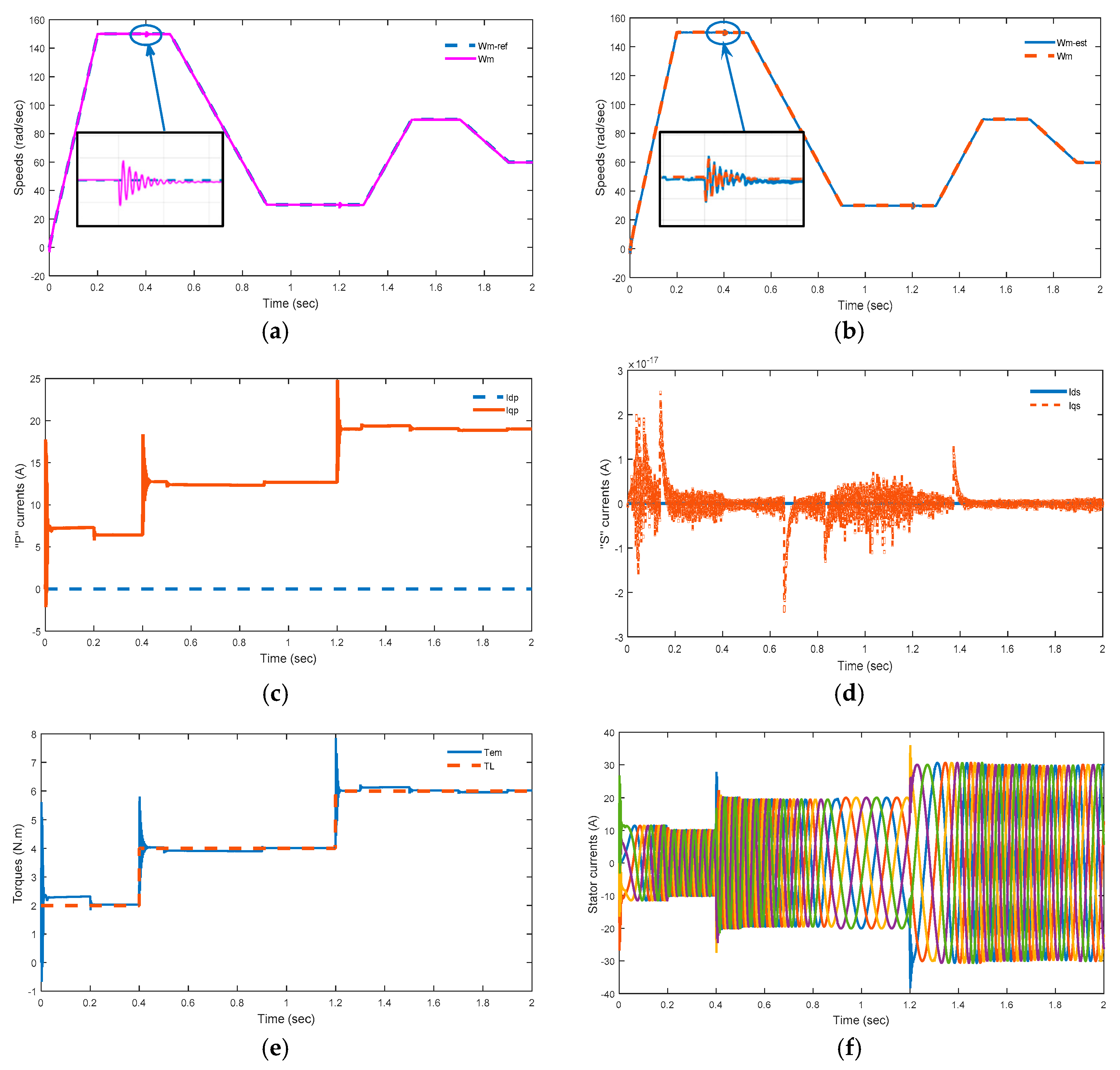
6.3.1. Healthy Operation Condition

The working performance of the 5P-PMSM in a closed-loop control system using backstepping control is studied in the case of no sensor fault in order to check the efficiency of the suggested SMO.

Figure 4. 5P-PMSM performance in normal operation condition. (a) Speed dynamics with load torque aplication; (b) measured and estimated speeds; (c) measured (d_p,q_p) current responses; (d) measured (d_s,q_s) current responses; (e) electromagnetic and load torque responses; (f) stator phases currents.

Figure 4. 5P-PMSM performance in normal operation condition. (a) Speed dynamics with load torque aplication; (b) measured and estimated speeds; (c) measured (d_p,q_p) current responses; (d) measured (d_s,q_s) current responses; (e) electromagnetic and load torque responses; (f) stator phases currents.

As indicated in Figure 4b,f, it is clear that the developed SMO is able to estimate the 5P-PMSM stator speed and currents well, and the error signals remain at a low value near zero. The proposed backstepping speed controller presents a high performance against load torque rejection. When the perturbation is applied to the system as the load torque or reference variation, the system fluctuations are small and the sliding mode response is quick. Figure 4c proves that the “d” and “q” current evolutions of the 5P-PMSM are maintain the FOC principle well. Figure 4d illustrates the secondary currents, which indicates that the performance of the FOC is well maintained. Figure 4 reveals the high closed-loop control system performance.

6.3.2. Fault Operation Condition

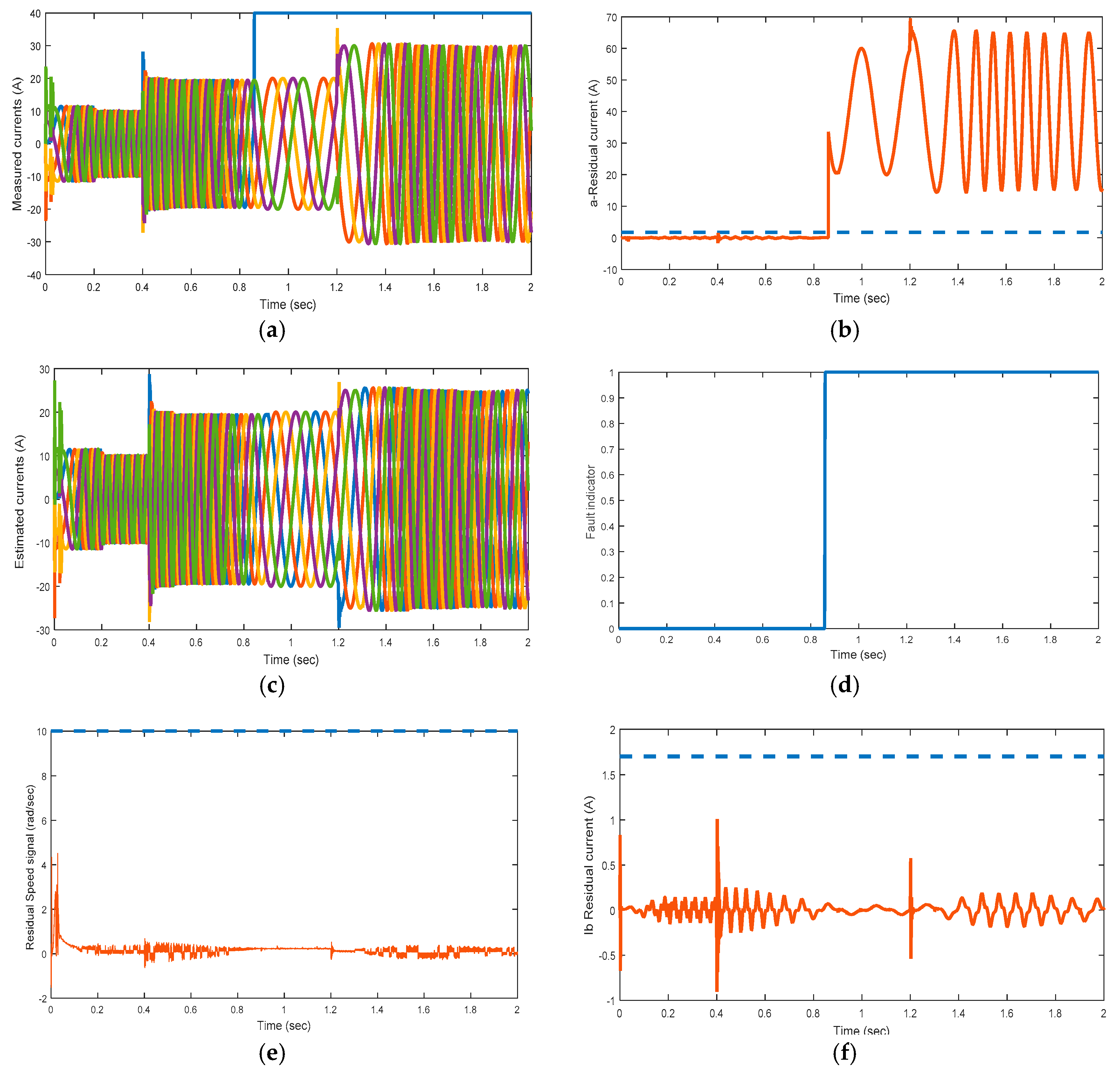
• Current Sensor fault in a-phase

In this simulation test, a sensor speed fault is chosen as a constant signal with K = 40 applied at t = 0.82 s when the a-phase current sensor is blocked, and the obtained simulation results are illustrated in Figure 5.

Figure 5. 5P-PMSM performance with constant fault applied in phase “a”. (a) Stator currents with a-phase fault application; (b) residual of a-phase current; (c) estimated stator currents; (d) fault indicator; (e) residual rotor speed; (f) residual b-phase current.

Figure 5. 5P-PMSM performance with constant fault applied in phase “a”. (a) Stator currents with a-phase fault application; (b) residual of a-phase current; (c) estimated stator currents; (d) fault indicator; (e) residual rotor speed; (f) residual b-phase current.

It can be pointed out from Figure 5a that, at t = 0.82 s, the actual a-phase stator current varies suddenly. However, the estimation of the other phase currents by the SMO is not affected, as shown in Figure 5c. As illustrated in Figure 5b, at t = 0.82 s, the a-phase error current is ${\epsilon }_{ia}=\left|i_a-{\widehat{i}}_a\right|>Threshold.$ Therefore, the fault indicator ${\mathsf{{\rm Y}}}_{ia}$ changes from 0 to 1, denoting a fault occurrence in the corresponding phase (Figure 5d). However, the b-c-d-e phases current sensors and the speed sensor are healthy and running normally, and the residual signals are away from the preset threshold, as is clearly noticed in Figure 5e,f. The fault indicator subsists at 0, which means that these signals are not touched by the faulted a-phase current sensor.

Thus, using the fault-tolerant algorithm, the closed-loop feedback signals (i_a-FTC, i_b-FTC, i_c-FTC, i_d-FTC, i_e-FTC, ω_m-FTC) can be obtained.

• Current Sensor constant fault in b-phase

In this simulation test, the constant fault applied to the b-phase sensor is K = 20 and the numerous simulation results are exhibited in Figure 6. These results are obtained with the load torque application at t = 0, t = 0.4 and t = 1.2.

Figure 6. 5P-PMSM performance with constant fault applied in phase “b”: (a) stator currents with b-phase fault application; (b) estimated stator currents; (c) residual of b-phase current; (d) fault indicator; (e) measured and estimated speeds; (f) measured (d_p,q_p) currents responses.

Figure 6. 5P-PMSM performance with constant fault applied in phase “b”: (a) stator currents with b-phase fault application; (b) estimated stator currents; (c) residual of b-phase current; (d) fault indicator; (e) measured and estimated speeds; (f) measured (d_p,q_p) currents responses.

As illustrated in Figure 6, in the failure occurrence at t = 0.9 s, a constant variation is applied to the measured b-phase current. However, from Figure 6a,e, the other currents (a, c, d and e) and the rotor speed are not affected and the estimated ones, as indicated in Figure 6b, are similar to those in the normal operation condition. For the b-phase current, the fault indicator in Figure 5d changed at the occurrence fault time.

Through the proposed fault-tolerant algorithm mentioned in Figure 3, the closed-loop feedback signals can be established as follows: i_b-FTC = 0 × i_b + 1 $\times {\widehat{i}}_b$, $i_{a-FTC}=i_a$, $i_{b-FTC}=i_b$, $i_{c-FTC}=i_c,$, $i_{d-FTC}=i_d$, $i_{e-FTC}=i_e$, $i_{\omega m-FTC}={\omega }_m$; thus, the feedback b-phase current switches from the actual to the estimated signal at the fault event corresponding to the fault algorithm equation mentioned above, whereas the other currents and speed feedback signals are constituted of the actual signals. Thus, the b-phase sensor fault does not engender heavy effects on the machine drive.

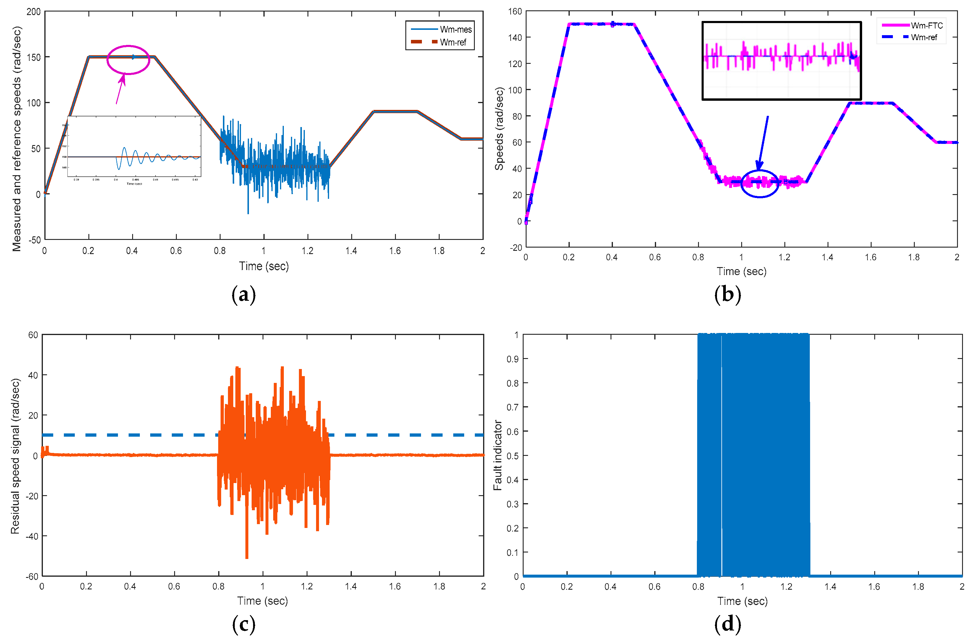
• Rotor speed Sensor noise fault

The simulation tests presenting the 5P-PMSM simulation responses are illustrated in Figure 7 for the noise fault rotor speed sensor case and in Figure 8 for the constant fault rotor speed sensor fault case.

In these simulation tests, the electromagnetic and the load torque are applied at t = 0 s, t = 0.4 s and at t = 1.2 s and the sensor fault is applied at t = 0.8 s in the first case and at t = 0.9 s in the second one.

The entire FTC scheme performance with the noise speed sensor failure, applied at t = 0.8 s, is mentioned in Figure 7. In Figure 7a,b, the SMO estimated rotor speed ${\omega }_{m-est}$, the measured speed ${\omega }_{m-mes}$ and the reconstructed speed ${\omega }_{m-FTC}$ with the proposed FTC strategy are presented. The fault noise and threshold fault indicator are shown in Figure 7c,d due to the speed sensor failure event, where the measured rotor speed is affected by noise. In Figure 7b, in the fault occurrence moment, the reconstructed speed with FTC tracks the reference and continues to follow it due to the switching algorithm, which enables it to replace the measured speed with the estimated one in the closed loop. Figure 7c demonstrates the preset rotor speed threshold and the residual rotor speed responsible for detecting the speed fault. Figure 7e,f show the actual primary and secondary quadratic currents. It can be proved that the generated control law achieves the FOC principle very effectively.

• Rotor speed sensor constant Fault

In Figure 8, the sensor offset failure is treated as a constant value. It is applied to the rotor speed during the operation sensor time. Figure 8a shows the motor speed response with a load torque application and speed sensor fault occurrence at t = 0.9 s. We can notice that the measured speed ω_m-mes is affected by the sensor fault, and that its value is deviated from the reference ${\omega }_m^{*}$.

Figure 8c illustrates the speed residue and the correlated threshold. Earlier to the fault event, the residue is 0, but, at t = 0.9 s, the speed residual rises and exceeds the threshold value, as indicated in Figure 8d.

Figure 7. 5P-PMSM performance with speed sensor noise fault: (a) speed responses with speed sensor fault occurrence at t = 0.8 s; (b) speed responses with FTC strategy; (c) fault noise and threshold (d) fault indicator; (e) primary current responses; (f) secondary current response; (g) measured stator currents; (h) estimated stator currents.

Figure 7. 5P-PMSM performance with speed sensor noise fault: (a) speed responses with speed sensor fault occurrence at t = 0.8 s; (b) speed responses with FTC strategy; (c) fault noise and threshold (d) fault indicator; (e) primary current responses; (f) secondary current response; (g) measured stator currents; (h) estimated stator currents.

Figure 8. 5P-PMSM performance with speed sensor constant fault: (a) speed dynamics with load torque application; (b) measured and estimated speeds with FTC; (c) residual speed signal and threshold; (d) fault indicator.

Figure 8. 5P-PMSM performance with speed sensor constant fault: (a) speed dynamics with load torque application; (b) measured and estimated speeds with FTC; (c) residual speed signal and threshold; (d) fault indicator.

• Two sensors a and b are affected with speed sensor constant fault

The results presenting the responses of the 5P-PMSM in the case of three sensor faults are illustrated in Figure 9. The faults applied in this case are a constant speed sensor fault and the “a” and “b” currents sensor faults. For the obtained simulation results, the electromagnetic and the load torque are carried out at t = 0 s, t = 0.4 s and t = 1.2 s and the sensor fault is implemented at t = 0.9 s for speed and b-phase sensor current faults and at t = 0.5 s for the a-phase sensor fault.

Figure 9. 5P-PMSM performance with speed and current sensor faults: (a) currents responses with fault application; (b) currents responses with FTC strategy application; (c) estimated currents; (d) speed responses with load torque and speed sensor; (e) stator current errors; (f) primary current responses; (g) secondary current responses; (h) electromagnetic and load torques.

Figure 9. 5P-PMSM performance with speed and current sensor faults: (a) currents responses with fault application; (b) currents responses with FTC strategy application; (c) estimated currents; (d) speed responses with load torque and speed sensor; (e) stator current errors; (f) primary current responses; (g) secondary current responses; (h) electromagnetic and load torques.

In Figure 9, the speed sensor offset fault is considered as a constant value with “a” and “b” current faults applied previously in simulation tests. This figure illustrates the motor speed and current dynamics in a faulty sensor case.

Figure 9b represents the currents responses with FTC strategy application. Earlier to the fault occurrence, this demonstrates the faults occurrence at t = 0.5 s for the a-phase current and at t = 0.9 s for b-phase current. The c, d and e phases currents are not subjected to the failure event.

Figure 9c confirms the drive observer efficiency. It is clear that the SMO displays a satisfactory current tracking behavior. Similarly, in Figure 9d, it is revealed that the disturbance (load torque) does not have an undesirable effect on the speed tracking control. This figure demonstrates the motor speed dynamics with a load torque application and speed sensor fault occurrence at t = 0.9 s, where ω_m-mes is the measured speed, ω_m-est is the estimated speed and ${\omega }_{m-FTC}$ is the reconstructed one. It can be noted that the sensor fault affects the measured speed ω_m-mes value, which is deviated from the reference ${\omega }_m^{*}$.

Figure 9h presents the electromagnetic and the load torques. It is clear that the motor drive is capable of surmounting the load disturbance and compensating for it thanks to the control current efficiency.

Figure 9f presents the measured and the estimated (d,q) 5P-PMSM currents’ evolution, which is efficiently monitored using the backstepping controller. Indeed, the secondary 5P-PMSM phase currents are given in Figure 9g, and are not modified or affected before and after the reconfiguration, and remain at zero in order to conserve the FOC principal control. The simulation tests show the effectiveness of the elaborated FTC strategy for a 5P-PMSM with speed and current sensor faults.

7. Discussion

In this research work, it is demonstrated that the proposed FTC scheme is able to surmount the sensor faults even for both speed and current sensors faults occurrence. Herein, the multiphase machine is tested for almost all of their sensors’ fault presence. Firstly, the current senor fault is considered for one phase and two phases. It is noticed that the current faults do not have an effect on the speed and electromagnetic responses. Secondly, others current sensors are healthy and operating normally because their fault indicators remain at zero.

In fact, for the affected current sensor, the feedback phase current switches from the actual to the estimated signal obtained from SMO at the fault event corresponding to the proposed FTC algorithm, whereas the healthy currents and speed feedback signals are still composed of the measured signals. Thus, the faulty sensor does not generate heavy effects on the machine drive.

For the speed sensor fault, two fault types are considered: the constant and the noise perturbance. For the constant fault, it is easily shown that, in the fault occurrence moment, the reconstructed speed with FTC follows the reference and continues to follow it due to the switching algorithm, which enables us to substitute the actual speed by the estimated one in the closed loop. For the noise perturbance fault, it is demonstrated that the magnitude oscillations are attenuated due to the choice of the threshold value responsible for detecting and mitigating the noise effects.

Indeed, several research works are interested in the FTC strategy by estimating the fault. In [19], the fault is estimated using the EID (equivalent input disturbance) estimator’s obtained estimate, which is incorporated into the state-feedback control law to compensate for the fault effect. In [38], the author deals with a current sensor fault reconstruction algorithm for the torque closed-loop drive system of an interior PMSM. The sensor faults are equated to actuator ones by a newly introduced state variable. Then, the phase current sensor faults are reconstructed by means of an adaptive method.

Most of the existing FTC schemes [5,6,7,8] focus on handling system faults by employing proportional integral (PI) controllers in the control-loops. For others [42], only the speed sensor fault is considered using the FTC strategy based on a HOSM observer (higher order sliding mode) for the three-phase PMSM. For the five-phase PMSM, the most studied fault is the open-circuit fault because it represents the most common type of faults in electric drives for high power system drives, and is crucial for continuing the drive operation under fault conditions.

In this work, it is important to note that the occurrence fault in one sensor type does not disturb the other signals, which means that the motor drive is capable of overcoming the internal (load torque) and external (sensor faults) perturbances, and compensates for them thanks to the effective control strategy based on the backstepping approach (for speed and current loops). Thus, it is important to mention that the FTC scheme developed is very attractive for dealing with more than one sensor fault at the same time.

8. Conclusions

This paper introduces a fault-tolerant control technique based on the 5P-PMSM SMO observer. The designed control scheme is developed in the presence of the speed and current sensor faults.

The FTC strategy is developed based on three main steps. First, the SMO is proposed for fault detection. Then, the rotor speed and stator current are estimated and continuously compared with the threshold in order to produce a residual signal for the fault detection block. Second, the reconstruction mechanism enables us to switch between measured and estimated speeds according to the fault-tolerant algorithm. Finally, velocity and current steady-state errors are sent to the backstepping controllers to determine the best tracking trajectory performance.

Numerical simulations executed under various operating and boundary conditions demonstrate that the developed FTC can attain a continuous 5P-PMSM operation.

This achievement is certainly a key issue of the improvement of energy conversion efficiency in motor drives. For future works, it is recommended that the FTC strategy can be exploited in the case of multiple faults, including actuator faults, when the 5P-PMSM is fed by a photovoltaic system, which will be highly beneficial for several industrial and agricultural applications.

References

1. Gong, J.; Zahr, H.; Semail, E.; Trabelsi, M.; Aslan, B.; Scuiller, F. Design Considerations of Five-Phase Machine with Double p/3p Polarity. IEEE Trans. Energy Conv. 2019, 34, 12–24. [Google Scholar] [CrossRef]
2. Hezzi, A.; Elghali, S.B.; Salem, Y.B.; Abdelkrim, M.N. Control of five-phase PMSM for electric vehicle application. In Proceedings of the 18th International Conference on Sciences and Techniques of Automatic Control & Computer Engineering—STA’2017, Monastir, Tunisia, 21–23 December 2017. [Google Scholar]
3. Li, L.; Ding, S.X.; Luo, H.; Peng, K.; Yang, Y. Performance-Based Fault-Tolerant Control Approaches for Industrial Processes with Multiplicative Faults. IEEE Trans. Ind. Inform. 2020, 16, 4759–4768. [Google Scholar] [CrossRef]
4. Kommuri, S.K.; Rath, J.J.; Veluvolu, K.C.; Defoort, M. Robust fault-tolerant cruise control of electric vehicles based on second-order sliding mode observer. In Proceedings of the 2014 14th International Conference on Control, Automation and Systems (ICCAS 2014), Gyeonggi-do, Korea, 22–25 October 2014; pp. 698–703. [Google Scholar] [CrossRef]
5. Yang, J.; Dou, M.; Zhao, D. Iterative sliding mode observer for sensoreless control of five-phase permanent magnet synchronous motor. Bulletin of the polish academy of sciences. Tech. Sci. 2017, 65, 845–857. [Google Scholar]
6. Nguyen, N.K.; Meinguet, F.; Semail, E.; Kestelyn, X. Fault-tolerant operation of an open-end winding five-phase PMSM drive with short-circuit inverter fault. IEEE Trans. Ind. Electron. 2016, 63, 595–605. [Google Scholar] [CrossRef] [Green Version]
7. Mohammadpour, A.; Sadeghi, S.; Parsa, L. A generalized fault-tolerant control strategy for five-phase PM motor drives considering star, pentagon, and pentacle connections of stator windings. IEEE Trans. Ind. Electron. 2014, 61, 63–75. [Google Scholar] [CrossRef]
8. Mohammadpour, A.; Parsa, L. A unified fault-tolerant current control approach for five phase PM motors with trapezoidal back EMF under different stator winding connections. IEEE Trans. Power Electron. 2013, 28, 3517–3527. [Google Scholar] [CrossRef]
9. Sadeghi, S.; Guo, L.; Toliyat, H.A.; Parsa, L. Wide operation speed range of five-phase permanent machines by using different stator winding configurations. IEEE Trans. Power Electron. 2012, 59, 2621–2631. [Google Scholar]
10. Hezzi, A.; Bensalem, Y.; Elghali, S.B.; Abdelkrim, M.N. Sliding mode observer sensoreless control of five-phase PMSM in electric vehicle. In Proceedings of the 19th International Conference on Sciences and Techniques of Automatic Control and Computer Engineering (STA), Sousse, Tunisia, 24–26 March 2019; pp. 530–535. [Google Scholar]
11. Tabrizchi, A.M.; Soltani, J.; Shishehgar, J.; Abjadi, N.R. Direct Torque control of Speed Sensorless Five-Phase IPMSM Based on Adaptive Input-Output Feedback Linearization. In Proceedings of the 5th Power Electronics, Drive Systems and Technologies Conference (PEDSTC 2014), Tehran, Iran, 5–6 February 2014. [Google Scholar]
12. Bensalem, Y.; Abbassi, R.; Jerbi, H. Fuzzy Logic Based-Active Fault Tolerant control of speed sensor failure for five phase PMSM. J. Electr. Eng. Technol. 2021, 16, 287–299. [Google Scholar] [CrossRef]
13. Hosseyni, A.; Trabelsi, R.; Iqbal, A.; Mimouni, M.F. Backstepping Control for a Five-Phase Permanent Magnet Synchronous Motor Drive. J. Power Electron. Drive Syst. 2015, 6, 842–852. [Google Scholar] [CrossRef]
14. Hosseyni, A.; Trabelsi, R.; Sanjeevikumar, P.; Iqbal, A.; Mimouni, M.F. Sensorless Back Stepping Control for a Five-Phase Permanent Magnet Synchronous Motor Drive Based on Sliding Mode Observer. In Advances in Power Systems and Energy Management; Lecture Notes in Electrical Engineering; Springer: Singapore, 2018; Volume 436. [Google Scholar] [CrossRef]
15. Jinpeng, Y.; Junwei, G.; Yumei, M.; Haisheng, Y. Adaptive Fuzzy Tracking Control for a Permanent Magnet Synchronous Motor via Backstepping Approach. Math. Probl. Eng. 2010, 2010, 391846. [Google Scholar]
16. Sobanski, P.; Ortowska-Kowalska, T. Detection of single and multiple IGBTs open-circuit faults in a field-oriented controlled induction motor drive. Arch. Electr. Eng. 2017, 66, 89–104. [Google Scholar] [CrossRef]
17. Kummuri, S.; Michael, D.; Karimi, H.R.; Veluvolu, K.C. A Robust Observer-Based sensor fault-tolerant control for PMSM in Electric Vehicules. IEEE Trans. Ind. Electron. 2016, 63, 7671–7681. [Google Scholar] [CrossRef]
18. Chen, H.; Jiang, B.; Ningyun, L. A Multi-mode Incipient Sensor Fault Detection and Diagnosis Method for Electrical Traction Systems. Int. J. Control Autom. Syst. 2018, 16, 1783–1793. [Google Scholar] [CrossRef]
19. Zhongyi, Y.; Yiguang, C. Interturn Short-Circuit Fault Detection of a Five-Phase Permanent Magnet Synchronous Motor. Energies 2021, 14, 434. [Google Scholar]
20. Li, T.; Ruiqing, M.; Zhen, Z. Diagnosis of open-phase fault of five-phase permanent magnet synchronous motor by harmonic current analysis. Microelectron. Reliab. 2021, 126, 114205. [Google Scholar] [CrossRef]
21. Gang, H.; Li, Z.; Edwardo, F.F.; Zhang, C.; He, J. An equivalent-input-disturbance approach for current sensor faults estimation and rejection in permanent magnet synchronous motor drives. Trans. Inst. Meas. Control 2020, 42, 365–373. [Google Scholar]
22. Kamila, J.; Mateusz, D. A Current Sensor Fault Tolerant Control Strategy for PMSM Drive Systems Based on Cri Markers. Energies 2021, 14, 3443. [Google Scholar]
23. Kummuri, S.; Veluvolu, K.C. Robust Sensors-Fault-Tolerance with Sliding Mode Estimation and Control for PMSM Drives. IEEE/ASME Trans. Mechatron. 2018, 23, 17–28. [Google Scholar] [CrossRef]
24. Klimkowski, K.; Dybkowski, M. An influence of the chosen sensors faults to the performance of the vector controlled induction motor drive system. Comput. Appl. Electr. Eng. 2014, 12, 294–301. [Google Scholar]
25. Yu, Y.; Zhao, Y.; Wang, B.; Huang, X.; Xu, D. Current Sensor Fault Diagnosis and Tolerant Control for VSI-Based Induction Motor Drives. IEEE Trans. Power Electron. 2018, 33, 4238–4248. [Google Scholar] [CrossRef]
26. Huang, G.; Huang, W.; Zhengtan, L.; Jiajun, L.; Jing, H.; Changfan, Z.; Zhao, K. An improved sliding-mode observer-based equivalent-input-disturbance approach for permanent magnet synchronous motor drives with faults in current measurement circuits. Trans. Inst. Meas. Control 2021, 43, 2589–2598. [Google Scholar] [CrossRef]
27. Jlassi, I.; Estima, J.; Khil, S.; Bellaaj, N.M.; Cardoso, A.J.M. A robust observer-based method for IGBTs and current sensors fault diagnosis in voltage-source inverters of PMSM drives. IEEE Trans. Ind. Appl. 2017, 53, 2894–2905. [Google Scholar] [CrossRef]
28. Khil, S.; Jlassi, I.; Estima, J.; Bellaaj, N.M.; Cardoso, A.J.M. Current sensor fault detection and isolation method for PMSM drives, using average normalised currents. IET Electron. Lett. 2016, 52, 1434–1436. [Google Scholar] [CrossRef]
29. Yin, S.; Luo, H.; Ding, S.X. Real-time implementation of fault-tolerant control systems with performance optimization. IEEE Trans. Ind. Electron. 2014, 61, 2402–2411. [Google Scholar] [CrossRef]
30. Tabbache, B.; Benbouzid, M.E.; Kheloui, A.; Bourgeot, J. Virtual sensor based maximum likelihood voting approach for fault tolerant control of electric vehicle powertrains. IEEE Trans. Veh. Technol. 2013, 62, 1075–1083. [Google Scholar] [CrossRef] [Green Version]
31. Tahri, A.; Said, H.; Moreau, S. A hybrid active fault-tolerant control scheme for wind energy conversion system based on permanent magnet synchronous generator. Arch. Electr. Eng. 2018, 67, 485–497. [Google Scholar]
32. Bunasla, N.; Barkat, S.; Benyoussef, E.; Tounsi, K. Sensoreless sliding mode control of a five-phase PMSM using Extended Kalman Filter. In Proceedings of the International Conference on Modeling, Identification and Control (ICMIC-2016), Algiers, Algeria, 15–17 November 2016. [Google Scholar]
33. Chakraborty, C.; Verma, V. Speed and current sensor fault detection and isolation technique for induction motor drive using axes transformation. IEEE Trans. Ind. Electron. 2015, 62, 1943–1954. [Google Scholar] [CrossRef]
34. Mateusz, D.; Kamil, K. Artificial Neural Network Application for Current Sensors Fault Detection in the Vector Controlled Induction Motor Drive. Sensors 2019, 19, 571. [Google Scholar] [CrossRef] [Green Version]
35. Kamil, K.; Mateusz, D. A Fault Tolerant Control Structure for an Induction Motor Drive System. Automatika 2016, 3, 638–647. [Google Scholar]
36. Mateusz, D.; Kamil, K. Stator current sensor fault detection and isolation for vector-controlled induction motor drive. In Proceedings of the IEEE International Power Electronics and Motion Control Conference (PEMC), Varna, Bulgaria, 25–28 September 2016. [Google Scholar]
37. Parsa, L.; Toliyat, H.A. Multi-phase permanent magnet motor drives. In Proceedings of the 38th IAS Annual Meeting on Conference Record of the Industry Applications Conference, Salt Lake City, UT, USA, 12–16 October 2003; Volume 1, pp. 401–408. [Google Scholar] [CrossRef]
38. Khan, M.R.; Iqbal, A. Experimental investigation of five-phase induction motor drive using extended Kalman-filter. Asian Power Electron. J. 2009, 3, 1–7. [Google Scholar]
39. Hosseyni, A.; Trabelsi, R.; Iqbal, A.; Padmanaban, S.; Mimouni, M.F. An improved sensorless sliding mode control/adaptive observer of a five-phase permanent magnet synchronous motor drive. Int. J. Adv. Manuf. Technol. 2017, 93, 1029–1039. [Google Scholar] [CrossRef]
40. Hezzi, A.; Elghali, S.B.; Bensalem, Y.; Zhibin, Z.; Benbouzid, M.; Abdelkrim, M.N. ADRC-Based Robust and Resilient Control of a 5-phase PMSM driven Electric Vehicle. Machines 2020, 8, 17. [Google Scholar] [CrossRef]
41. Qinyue, Z.; Zhaoyang, L.; Xitang, T.; Xie, D.; Dai, W. Sensors Fault Diagnosis and Active Fault-Tolerant Control for PMSM Drive Systems Based on a Composite Sliding Mode Observer. Energies 2019, 12, 1695. [Google Scholar] [CrossRef] [Green Version]
42. Jiwen, Z.; Lijun, W.; Liang, X.; Fei, D.; Juncai, S.; Xing, Y. Uniform Demagnetization Diagnosis for Permanent Magnet Synchronous Linear Motor Using a Sliding-Mode Velocity Controller and an ALN-MRAS Flux Observer. IEEE Trans. Ind. Electron. 2021, 69, 890–899. [Google Scholar]
Figure 1. Five-phase Voltage Source Inverter (VSI) topology.
Energies 15 00071 g001
Figure 2. The designed FTC strategy for 5P-PMSM.
Energies 15 00071 g002