A Two-Level Model Predictive Control-Based Approach for Building Energy Management including Photovoltaics, Energy Storage, Solar Forecasting and Building Loads

Abstract

This paper uses a two-level model predictive control-based approach for the coordinated control and energy management of an integrated system that includes photovoltaic (PV) generation, energy storage, and building loads. Novel features of the proposed local controller include (1) the ability to simultaneously manage building loads and energy storage to achieve different operational objectives such as energy efficiency, economic cost efficiency, demand response and grid optimization through the design of specific power trajectory tracking performance functionals, (2) an energy trim function that minimizes the impact of solar forecasting errors on system performance, and (3) the design of a state of charge controller that uses day-ahead forecast of solar power and building loads to intialize energy storage at the start of each day. The local controller is tested in simulation using an exemplary system with PV generation, energy storage and dispatchable building loads. Two sample days with different PV forecasts and multiple case scenarios are considered, and the performance of the algorithm in managing the real and reactive net building load trajectories and the ramp rate of PV injections into the utility network are evaluated. The simulations are based on actual forecasted and measured PV data, and the results show that the local controller meets the tracking requirements for real and reactive power within the operating constraints of the building.

1. Introduction

This paper presents the design of a two-level control system that includes a system controller and local controller, to manage real and reactive building power consumption and PV ramp rate for a building with rooftop PV and energy storage.

The variability of solar irradiance can create fluctuations and high ramp rates in photovoltaic (PV) generated power. The intermittency of PV generated power is a significant factor limiting the large-scale integration of PV and this issue has been investigated in the literature since the 1980’s [1,2], and is still being discussed [3]. The most common approach for PV ramp rate control is using energy storage devices to smooth out the fluctuations [4,5,6,7,8,9]. Energy storage can be used for supply-demand balancing by storing excess energy for future use or injecting power to the grid when PV cannot generate sufficient power due to poor weather conditions. Although this can increase the stability and reliability of the overall system, due to limited energy storage capacity the storage device may reach its maximum/minimum allowable state of charge during critical times of its operation. For example, due to such operating constraints the energy storage system may be unavailable to assist with PV ramp rate management and this can have significant negative impacts on distribution system operations. The traditional approach to ramp rate control is to use a moving average method [4,6,7,8,9,10]. Although this method can reduce PV output fluctuations, it cannot necessarily limit the PV ramp rate to be within a specific operating range [9]. In this paper, we propose a local control system based on model predictive control (MPC) for coordinated energy management and ramp rate control that addresses some of the major limitations of previous work and also adds a new dimension, the dynamic management of dispatchable building loads.

The two main objectives of our proposed algorithm are: (1) Implement efficient and orderly control of adjustable resource clusters on the energy-consumption side while absorbing power supply resources on the nearby distribution network side to solve urgent power management problems and increase the value of organizational collaboration. (2) Develop an energy internet strategy that includes the allocation of energy storage capacity to enable small microresources to participate in power ancillary services and support the in-depth development of power market reform. The proposed control system operates by enabling dispatchable renewable distributed generation through coordinated dynamic adjustment of building loads and the charging and discharging of a battery energy storage system. The building is connected to a feeder with other buildings, and the system-level controller manages the power flows within the feeder. Selecting the performance function of the proposed optimal control approach is an important element, as it defines the global purpose of our proposed algorithm. These purposes are generally related to energy efficiency [11,12], economic cost efficiency [13,14], demand response [15,16], grid optimization [17,18], etc. Note, using a performance function related to economic cost efficiency does not necessarily lead to a control system that promotes energy efficiency, and vice versa. The control system developed in this work is focused on minimizing the difference between the desired power trajectory of the building and the actual power trajectory of the building. In this way, the proposed control method can be used to achieve many different building performance objectives through the design of the desired power trajectory. According to the proposed control deign approach, based on the overall operational objectives at the system-level, the system controller defines target real and reactive power set points over a given time period (the desired power trajectories) for the buildings, and this information is provided to the local controllers for each of the buildings. The local controllers then coordinate the external generation from solar panels with the available storage in the battery and the controllable building loads to achieve the targeted set point requested by the system controller while satisfying building operating constraints. An economic (cost) operational objective can be achieved by selecting an objective function at the system-level that minimizes the total cost of energy, and translating this into real and reactive power trajectories for the buildings that are involved. The control method can also be modified such as to reduce building energy consumption during the peak hours, move energy consumption to off-peak times such as weekends or nighttime, or to support grid services such as voltage regulation, power flow management, and power factor correction. The flexibility that the proposed control approach provides can be of particular interest for systems with renewable energy resources such as wind and solar along with energy storage unit. The excess energy can be stored in the battery during off-peak hours and then used during peak hours. We can also consider a multi-objective approach where the dynamic operation of the buildings is guided by different objective functions during the day. For example, the proposed control system can responds to the energy efficiency for the first two hours of the day, cost efficiency for the next hour and grid optimization for the rest of the day.

To demonstrate the effectiveness of the two-level control system that has been developed, we provide a detailed simulation study to evaluate the control system in this paper. The system is currently deployed and operational at the Case Western Reserve University (CWRU) campus. One building on the CWRU campus has been equipped with a 50 kW roof top PV array and a 50 kW/200 kWh battery each with their own smart inverters that are connected at the AC bus, and a local control system based on MPC that dynamically manages PV ramp rate to achieve set point tracking of real and reactive power trajectories for the building as provided by the system controller. The local controller tracks the system controller set points through coordinated real-time control of building loads and energy storage. Details on the design, deployment, and operational performance of this system on the CWRU campus will be provided in a subsequent paper.

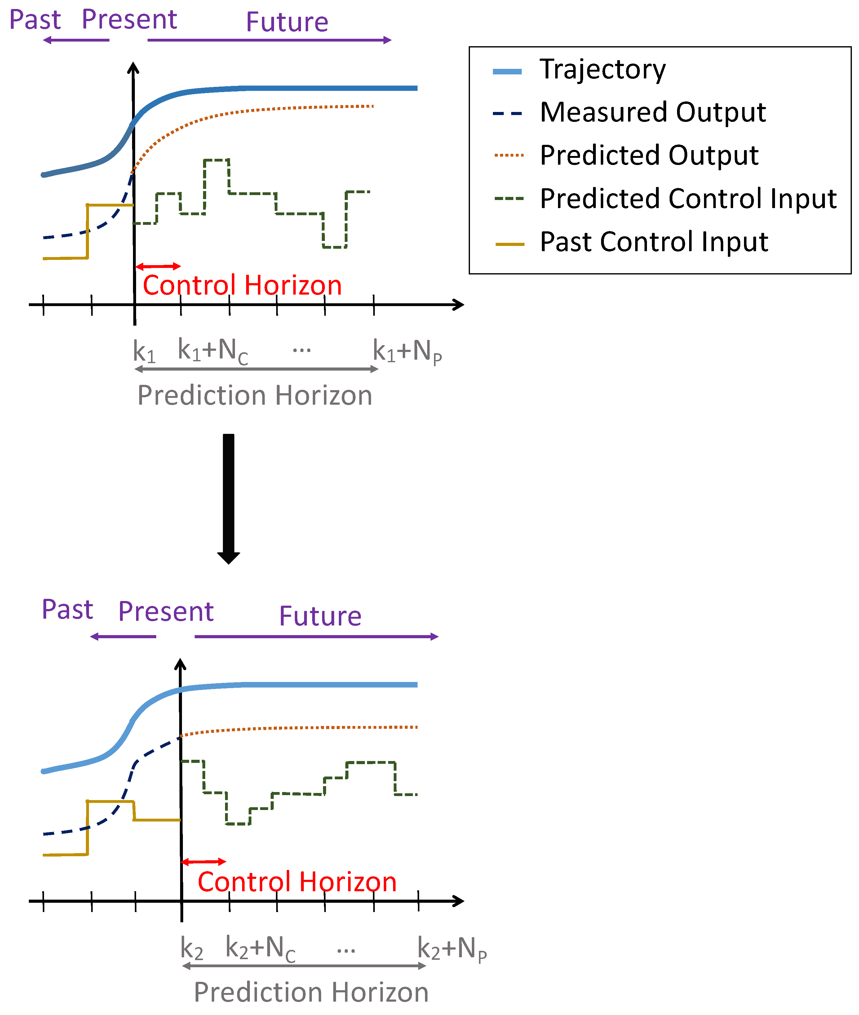
2. Model Predictive Control (MPC)

MPC was introduced for chemical process control in the late 1970s [19]. Recently, it has become a popular choice for many applications, including power systems; e.g., (1) as a ramp rate controller in wind turbines [20,21], (2) for controlling battery energy storage (BES) systems in conjunction with photovoltaic (PV) for smoothing solar injections [22] with a demonstrated reduction in cost and improvements in overall system performance without addressing ramp rate and PV forecasting errors in the system, (3) a MPC-based controller for reducing demand charges while increasing PV utilization without consideration of PV ramp rate constraints [23].

MPC control benefits from both optimal control and feedback, the controlled system can take proper actions to reduce the effects of negative actions before they occur based on predictions of inputs, disturbances and the future behavior of the system. The MPC controller can also take into account multiple objectives, and system limitations and constraints [24].

The MPC controller uses a receding horizon approach to solve for the optimal solution over a fixed time horizon into the future, i.e., the prediction horizon, using windowed local measurements and predictions while satisfying current and future system operational constraints. In the receding horizon strategy, the first element of the optimal control sequence in the control horizon is applied to the system, the system response is measured, and computations for the next prediction horizon are initiated. As the controller calculates the optimal solution for each prediction horizon, it is dynamically adjusting to the current system behavior and characteristics using a prediction model for the system. Predictions that can capture the general behavior of the system are sufficient for MPC controller design and deployment. Acceptable MPC performance can be obtained even with simple dynamic models and limited computational resources and measurements.

In this paper, we develop a novel approach based on MPC for controlling the PV ramp rate while responding to real and reactive power requests from system operators. The State of Charge (SoC) of the energy storage battery is also managed to prevent the battery from over charging/discharging during peak operating conditions. The MPC control design is formulated as a convex optimization problem that performs far better than traditional methods [25,26], and only requires local measurements and predictions over the prediction horizon window and does not require any further data from the utility distribution network the building is connected to. Another advantage of our algorithm over existing algorithms is the day-ahead prediction of battery usage to set the SoC at the beginning of each operating day. In general, the battery starts the day fully charged, or at a fixed level of $50\%$ SoC independent of anticipated operating conditions during that day. Then, on an overcast day for example, sufficient energy may not be available in the battery at mid-day and the system will no longer be able to control PV ramp rate or possibly meet the requested power targets from the system controller. On a very sunny day, the battery may not have sufficient charging capacity to store excess PV power as needed to meet requested power requirements for the system at a later time. In our approach, the battery is charged only to the level that is adequate for that day based on PV, building load and system load forecasts for the day. This eliminates battery overcharging, reduces the cost of the overall system, and increases the productivity of the system in poor weather conditions. Finally, the local controller also includes an ES (Energy Storage) trim function that dynamically adjusts the control commands to the energy storage system to eliminate errors due to the mismatch between predicated and actual PV data.

Other novelties and innovations of our proposed control approach include (1) a predictive control algorithm that simultaneously considers ramp rate control of the aggregated building power and following the set points requested from the system controller, and (2) dynamic management of building load at a slower time scale along with energy storage on a faster time scale to achieve overall management of building power. The majority of the literature has not considered ramp rate control in conjunction with the economic cost efficiency, energy efficiency or other grid-related objectives, or the integrated control of building loads in conjunction with PV and energy storage. The authors in [11] propose an energy management strategy for a residential microgrid with PV, wind turbine and solar thermal collectors. A battery energy storage system and water heater unit are used for a two-degree of freedom control strategy to reduce the overall system cost while balancing energy generation and consumption. Their control strategy does not consider the ramp rate control and the battery’s state of charge (SoC) is kept at $50\%$, without considering overnight calculations and next day predictions. Additionally, the power of the battery is considered as the difference between the net power and grid power, and the control algorithm does not dynamically manage dispatchable loads to control the load demand or use predictions of consumption. Ref. [27] develops a MPC strategy for demand response control of a building with HVAC system, PV panels and an energy storage system. Their objective is to minimize the total cost and reduce the load ramp rate, not the aggregated power ramp rate. A thermal model of the building is used without considering any energy consumption. Moreover, the battery’s SoC is maintained at $70\%$ without considering the next day predictions and overnight calculations. Finally, the authors in [13] have developed a sampling-based MPC control for a PV-integrated energy storage system to reduce the total cost of the energy of the entire system. All of these papers have failed to adequately address the complete problem including ramp rate control of the aggregated power along with managing load demand and consumption to achieve a more dynamic and efficient control of integrated (PV, energy storage, building load) system.

3. System Design and Modeling

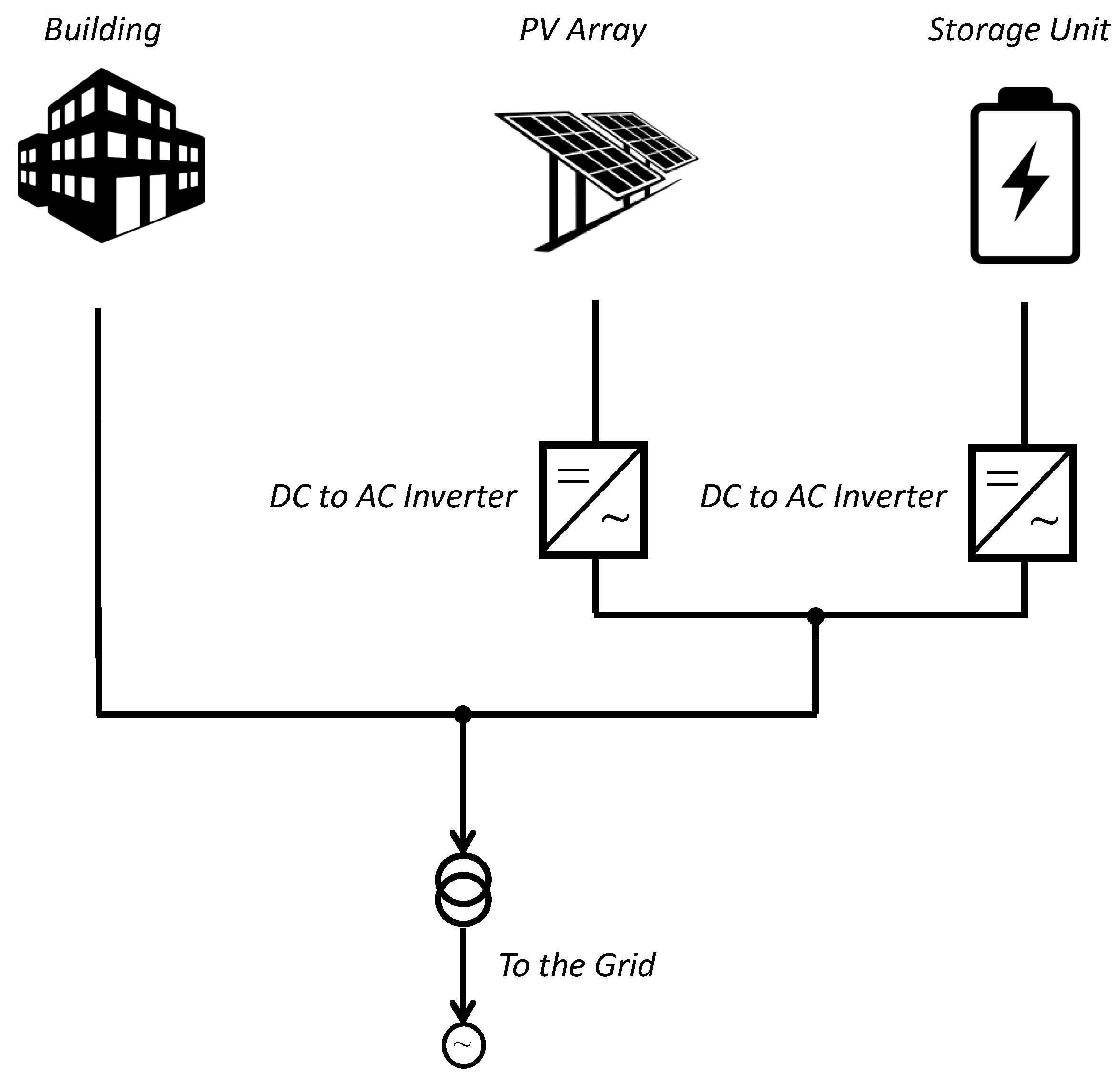
3.1. System Components and Dynamics

The schematic of the system we are considering in this paper is shown in Figure 1. The storage unit and PV array have separate DC to AC inverters and are connected at the AC side of the inverter. The power from the system is assumed positive when it is being supplied and is assumed negative when it is being consumed. The system components are as follows:

1.

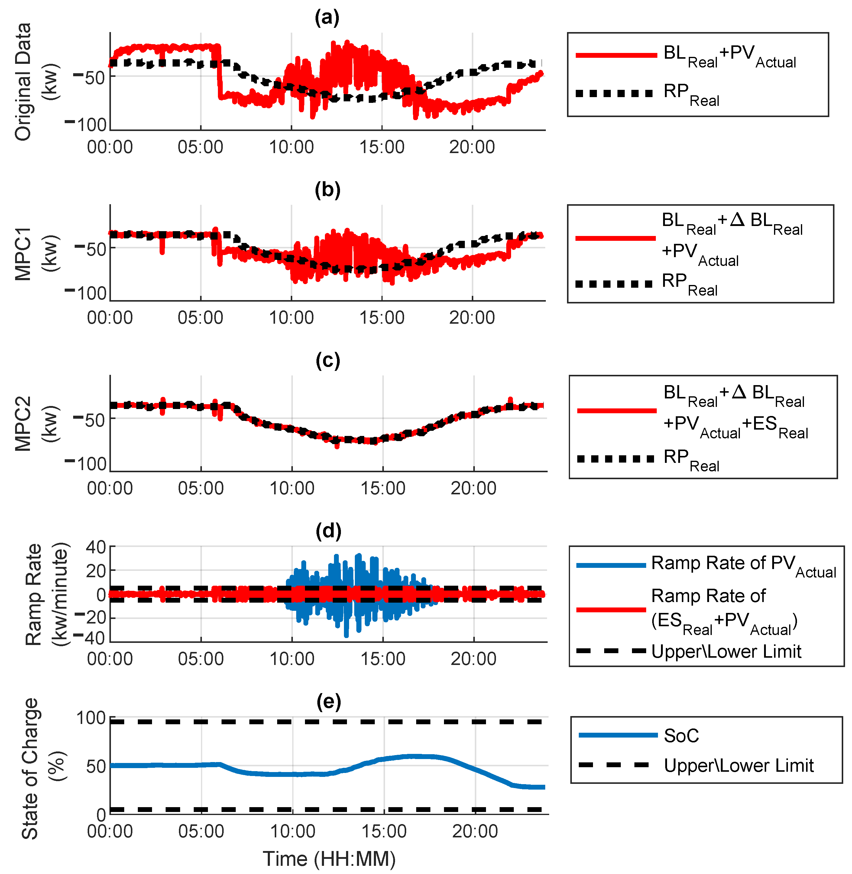
Photovoltaic (PV) Array: The power from this unit is always positive and the generated power has fluctuations due to weather conditions and is uncontrollable. The energy storage device is used for smoothing the PV fluctuations by limiting the ramp rate of generated power from the PV and battery to less than $10\%$ per-minute of installed PV capacity, as given by the Equation (1):

$$-10\%P{V}_{max}\le \mathrm{Ramp}\mathrm{Rate}\left(ES\left[t\right]+PV\left[t\right]\right)\le 10\%P{V}_{max}$$

(1)

where at time t, $ES\left[t\right]$ is the energy storage power (kW), $PV\left[t\right]$ is the generated PV power (kW) and $P{V}_{max}$ is the installed PV capacity (kW).

2.

Energy Storage (ES): This unit can charge and discharge, so the power can be both positive and negative. To maintain high efficiency, the charge/discharge rate and SoC per-minute are limited as follows:

$$\begin{array}{cc}\hfill & E{S}_{min}\le ES\left[t\right]\le E{S}_{max}\hfill \\ \hfill & So{C}_{min}\le SoC\left[t\right]\le So{C}_{max}\hfill \end{array}$$

(2)

where $ES\left[t\right]$ is the energy storage power at time t, $E{S}_{min}$ and $E{S}_{max}$ are lower and upper bound power limits, respectively, $So{C}_{min}$ and $So{C}_{max}$ are usable bounds for SoC, and $SoC\left[t\right]$ is the state of charge at time t minutes, a unitless value between $[0,1]$, calculated hourly by (3) with $ESCapacit{y}_{max}$ as the maximum capacity of the energy storage unit (kWh).

$$SoC\left[t\right]=SoC[t-1]-\frac{ES\left[t\right]}{60\times ESCapacit{y}_{max}}$$

(3)

3.

Building Load (BL): This building only consumes power, so the power is always negative. The total building load can be divided into controllable and uncontrollable loads, where the uncontrollable building loads are measured each minute and the controllable building loads are managed through the building control system using our proposed control method. For the controllable loads, dynamic models that capture the temporal behavior of how the load responds to changes in the set points (e.g., the response of changes in zone temperature set points and static pressure set points on HVAC loads) are included along with operational constraints that determine upper and lower bounds on acceptable changes to these controllable building loads over specified time periods (e.g., these bounds are based on their impact on building operating variables and occupants, such as zone temperatures and building pressure).

3.2. The MPC-Based Control Method

The main objective of the MPC-based local controller is to calculate a sequence of future control signals for building load and energy storage over a prediction horizon, $N_p$, such that the performance requirements and operating requirements are met. The control signals are calculated within a control horizon, $N_c\le N_p$, and based on the receding control horizon approach the first element of the control signal is applied within the control horizon, the initial conditions are updated, and the controller moves to the next prediction horizon, see Figure 2. The top figure shows the control and prediction horizons at time $k_1$, while the bottom figure shows the next prediction horizon, with time $k_2=k_1+N_c$.

At each time k, the controller is attempting to regulate the real (P) and reactive (Q) building load powers $\left\{B{L}_P\left[k\right],B{L}_Q\left[k\right]\right\}$, and real and reactive energy storage powers $\left\{E{S}_P\left[k\right],E{S}_Q\left[k\right]\right\}$, within their operating constraints to reduce the tracking error ($\left\{E_P\left[k\right],E_Q\left[k\right]\right\}$) between requested power ($\left\{R{P}_P\left[k\right],R{P}_Q\left[k\right]\right\}$) and the total building power ($\left\{P_{Total}\left[k\right],Q_{Total}\left[k\right]\right\}$):

$$\begin{array}{cc}\hfill & E_P\left[k\right]=R{P}_P\left[k\right]-P_{Total}\left[k\right],\hfill \\ \hfill & E_Q\left[k\right]=R{P}_Q\left[k\right]-Q_{Total}\left[k\right],\hfill \end{array}$$

(4)

where

$$\begin{array}{cc}\hfill & P_{Total}\left[k\right]=B{L}_P\left[k\right]-E{S}_P\left[k\right]-PV\left[k\right],\hfill \\ \hfill & Q_{Total}\left[k\right]=B{L}_Q\left[k\right]-E{S}_Q\left[k\right].\hfill \end{array}$$

(5)

Note that PV only generates real power and because there are uncertainties associated with the actual PV power generation, for example due to weather, $PV\left[k\right]=P{V}_{forecast}\left[k\right]$ is used in Equation (5) to develop the following (predictive) control strategy:

$$\begin{array}{cc}\hfill & E_P\left[k\right]=R{P}_P\left[k\right]-\left(B{L}_P\left[k\right]-E{S}_P\left[k\right]-P{V}_{forecast}\left[k\right]\right)\hfill \\ \hfill & E_Q\left[k\right]=R{P}_Q\left[k\right]-\left(B{L}_Q\left[k\right]-E{S}_Q\left[k\right]\right)\hfill \end{array}$$

(6)

The optimization problem in the control method is then solved in two steps, denoted by MPC1 and MPC2. MPC1 controls the large slower moving building loads for total power shifting while MPC2 controls the smaller fast charging unit, energy storage, for smoothing and to address any deficits that cannot be met by MPC1 on the appropriate time-scales.

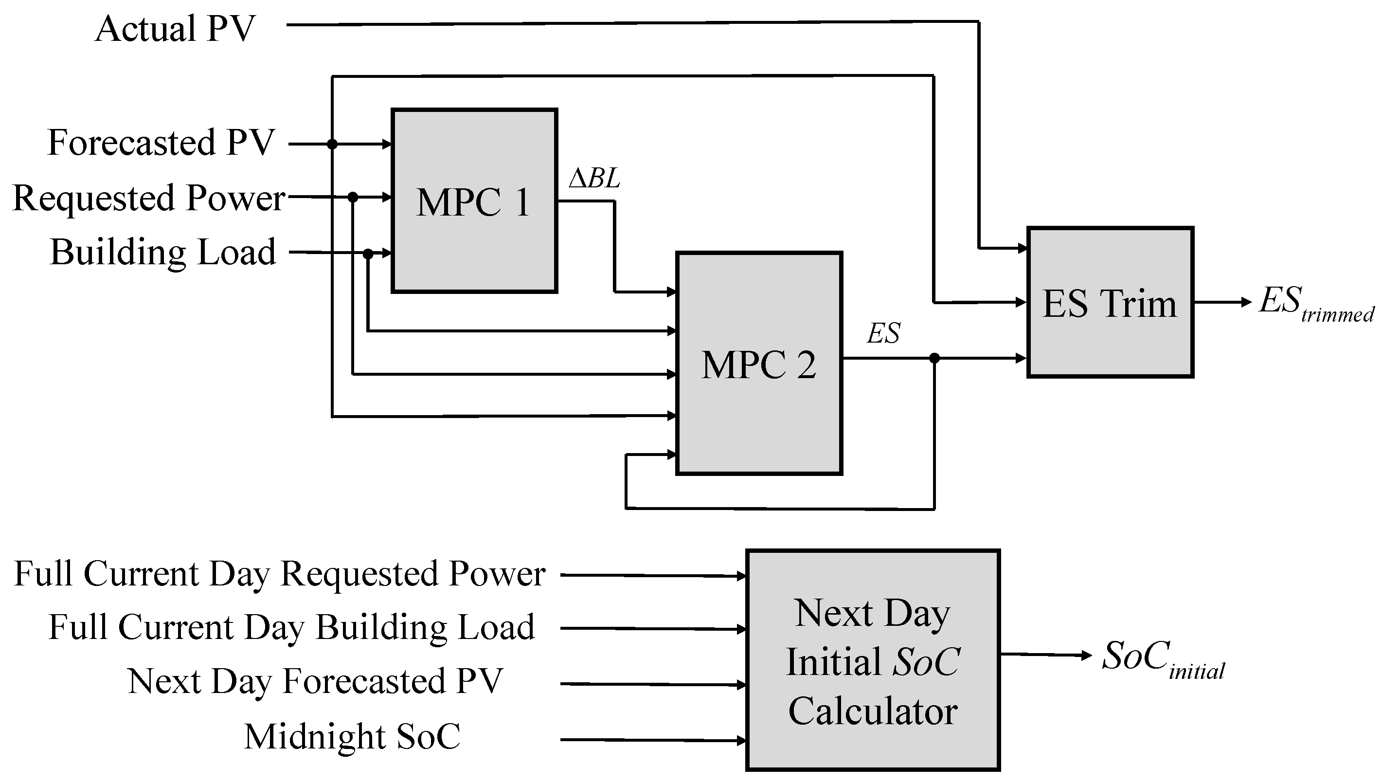
3.3. Local Controller Design

Figure 3 shows the block diagram of the local controller. The system consists of seven data blocks, (Required Power, PV Forecast, PV Actual, Building Load, SoC, Next Day PV Forecast, Next Day Forecasted Building Load), two optimization blocks, (MPC1, MPC2), and two calculation blocks (ES Trim, Next Day Initial SoC Calculator). Prediction models for the energy storage and building load are used inside the MPC1 and MPC2 blocks to predict real and reactive energy storage power and building load within a given time horizon. The optimization and calculation block are as follows:

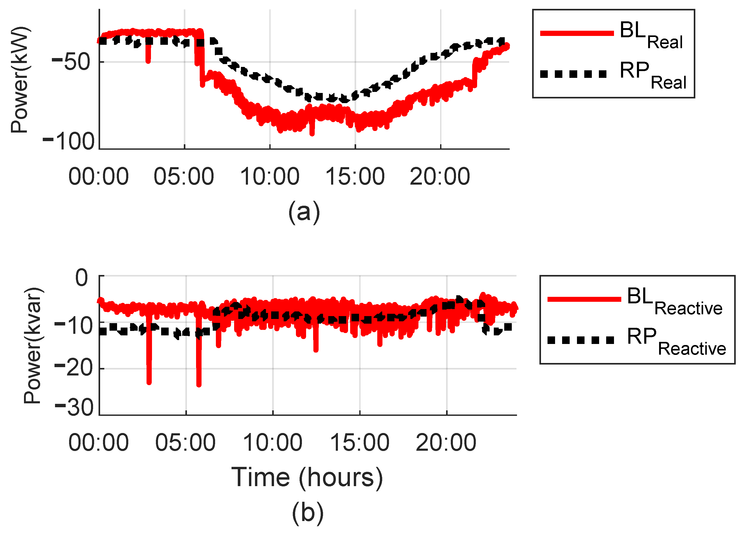
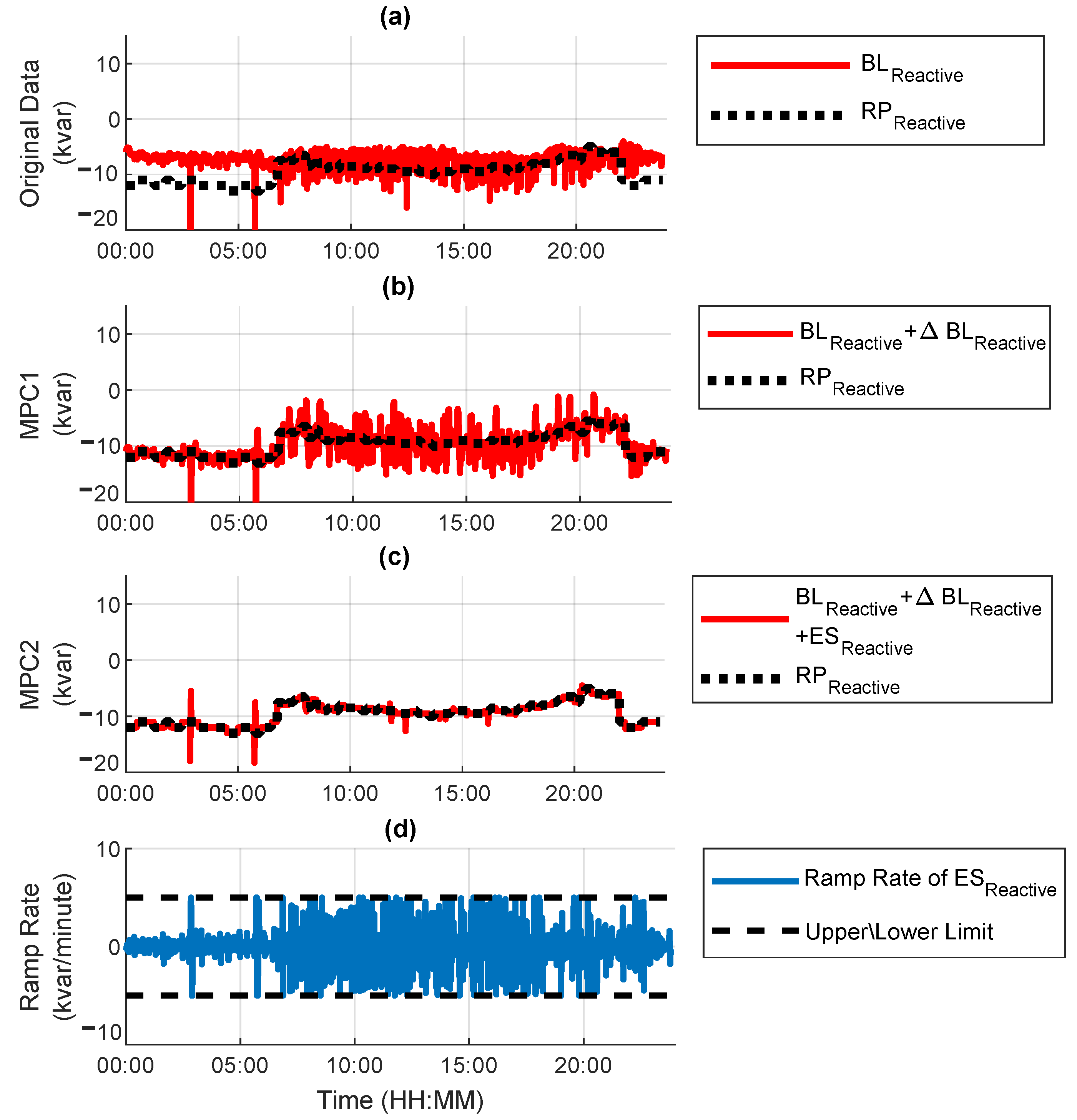
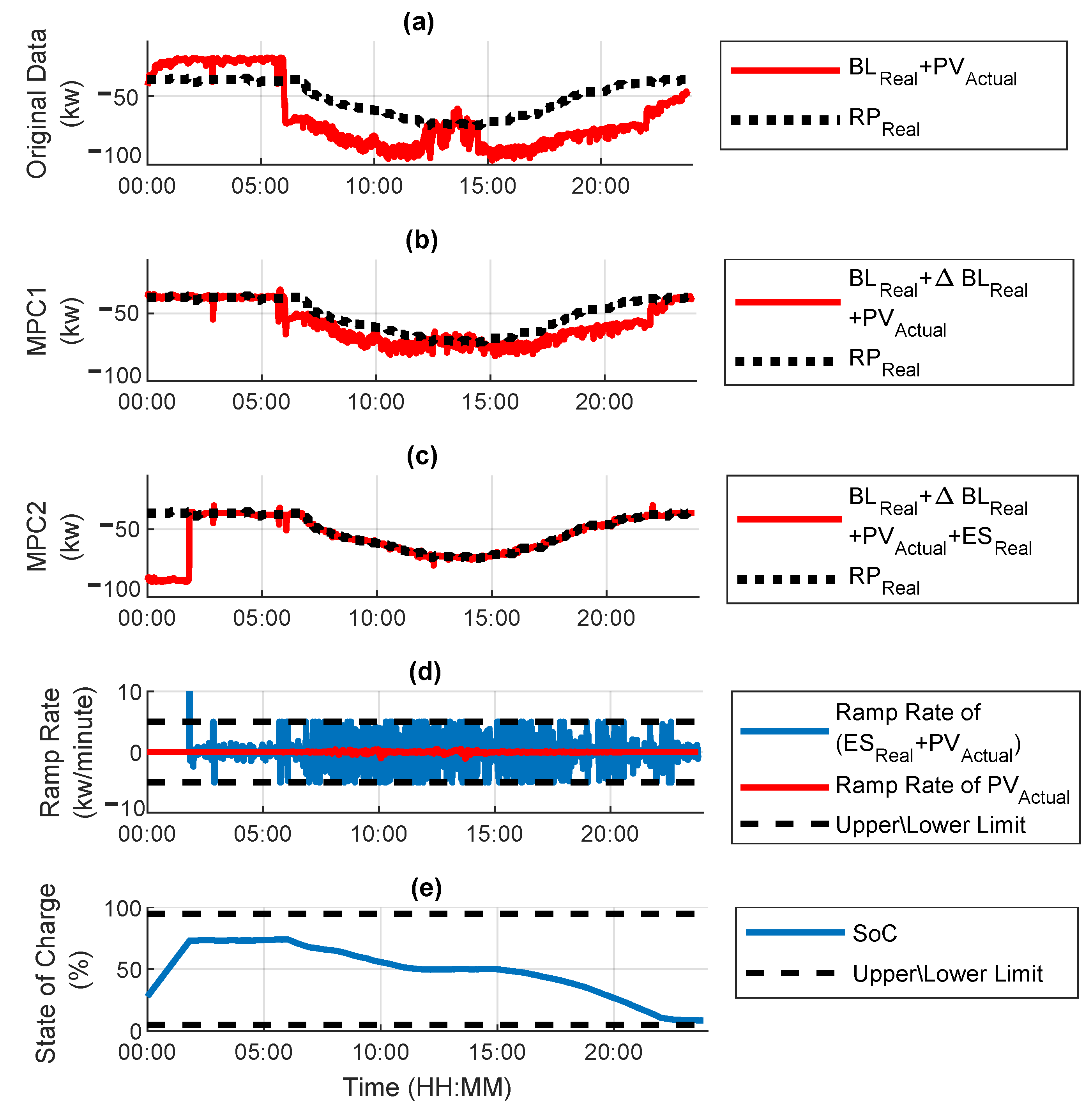
• MPC1: This block calculates the optimized real and reactive building load that minimizes the difference between the requested power and the sum of PV forecast and building load at each time step k within the building operating constraints and a given time horizon.
• MPC2: This block calculates the real and reactive energy storage power that maintains the per minute ramp rate constraint for the combined PV forecast and energy storage power, assists with minimizing the difference between the requested power and the sum of PV forecast and building load at each time step k, while satisfying energy storage system operating constraints and maintaining SoC within its required operating limits.
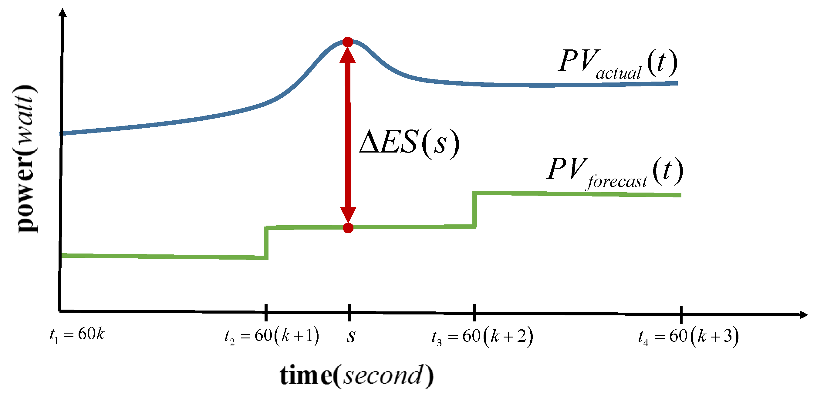
• ES Trim: This block modifies the energy storage power to eliminate the impact of PV forecasting errors on the response of the local (MPC2) controller.
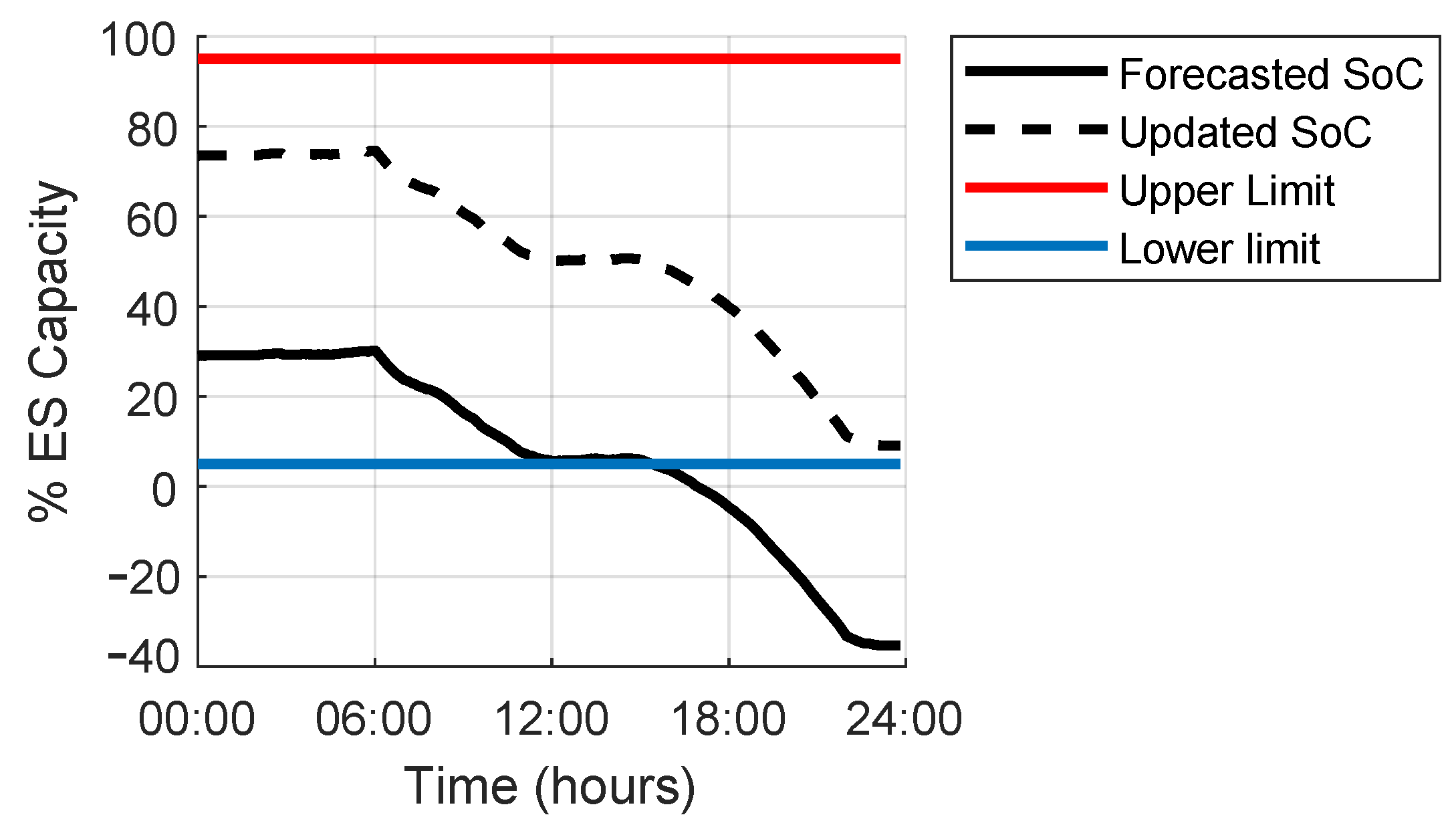
• Next Day Initial SoC Calculator: This block calculates the predicted initial SoC to meet the forecasted energy requirements (requested building load power given predicted building loads and PV forecast) for the next day.

The MPC controller structure, as shown in Figure 3, is a two-layer hierarchical structure with MPC1 in the first layer and MPC2 and ES Trim in the second layer. The first layer, MPC1, manages the building load system with slower dynamics as compared to the fast-responding battery controlled by MPC2 in the second layer. Multi-layer control structures are widely used in controlling large-scale systems where the system has multiple subsystems that operate on different time-scales. Interested readers can refer to [28] and the references therein for more details and examples on application of MPC to two-layer hierarchical control systems.

3.3.1. MPC1 (Building Load Calculations)

Consider the building load prediction horizon $N_{p,BL}$, control horizon $N_{c,BL}$, sliding prediction window $p{w}_{BL}=[t,t+N_{p,BL}]$, and control window $c{w}_{BL}=[t,t+N_{c,BL}]$, for the Building Load (BL) MPC controller. The prediction window slides through data for every $N_{c,BL}$ time period. Within each window, the optimization problem in (7) is solved for the optimal building load control input to the building load, $u_{BL}^{*}\left(p{w}_{BL}\right)=\left[u_{P,BL}^{*}\left(p{w}_{BL}\right),u_{Q,BL}^{*}\left(p{w}_{BL}\right)\right]$, that minimizes the cost function $J_1$ within the given operational constraints. The quadratic cost function $J_1$ minimizes the tracking error and is defined as the error between the requested power and the sum of the forecasted PV and building load. The optimal control for BL is computed within the control window, $u_{BL}^{*}\left(c{w}_{BL}\right)=\left[u_{P,BL}^{*}\left(c{w}_{BL}\right),u_{Q,BL}^{*}\left(c{w}_{BL}\right)\right]$, and this is then used to calculate the BL setpoint for the control window, $BL\left(c{w}_{BL}\right)=\left[B{L}_P\left(c{w}_{BL}\right),B{L}_Q\left(c{w}_{BL}\right)\right]$ and the initial states for the next prediction window, $X_{BL}(p{w}_{BL}+1)$$=\left[X_{P,BL}(p{w}_{BL}+1),X_{Q,BL}(p{w}_{BL}+1)\right]$ where $p{w}_{BL}+1=[t+N_{c,BL},t+N_{c,BL}+N_{p,BL}]$. The prediction window continues sliding until the end of the given operational period.

$$\left\{\begin{array}{cc}\hfill & {{\displaystyle \underset{u_{BL}^{*}\left(p{w}_{BL}\right)}{min}}}_{}{J}_1={\displaystyle \sum _{t\in p{w}_{BL}}}\left\{{\left[f_P,f_Q\right]}^{T}R\left[f_P,f_Q\right]\right\}\hfill \\ \hfill & \\ \hfill & s.t.\hfill \\ \hfill & 1.BLModel\left\{\begin{array}{cc}\hfill & X_{BL}[t+1]=A_{BL}{X}_{BL}\left[t\right]+B_{BL}{u}_{BL}\left[t\right]\hfill \\ \hfill & Y_{BL}\left[t\right]=C_{BL}{X}_{BL}\left[t\right]\hfill \end{array}\right.\hfill \\ \hfill & 2.\stackrel{}{}min\left(BL\right)\le BL\left[t\right]\le max\left(BL\right)\hfill \end{array}\right.$$

(7)

where

$$\left\{\begin{array}{cc}\hfill & f_P=R{P}_P\left[t\right]-\left(B{L}_P\left[t\right]+P{V}_{forecast}\left[t\right]\right),\hfill \\ \hfill & f_Q=R{P}_Q\left[t\right]-B{L}_Q\left[t\right],\hfill \\ \hfill & X_{BL}\left[t\right]=\left[\begin{array}{c}{X}_{B{L}_P}\left[t\right]\\ X_{B{L}_Q}\left[t\right]\end{array}\right],u_{BL}\left[t\right]=\left[\begin{array}{c}{u}_{B{L}_P}\left[t\right]\\ u_{B{L}_Q}\left[t\right]\end{array}\right],\hfill \\ \hfill & Y_{BL}\left[t\right]=\left[\begin{array}{c}BL\left[t\right]\\ BL[t+1]\end{array}\right],A_{BL}=\left[\begin{array}{cc}{A}_{B{L}_P}& 0\\ 0& A_{B{L}_Q}\end{array}\right],\hfill \\ \hfill & B_{BL}=\left[\begin{array}{cc}{B}_{B{L}_P}& 0\\ 0& B_{B{L}_Q}\end{array}\right],C_{BL}=\left[\begin{array}{cc}{C}_{B{L}_P}& 0\\ 0& C_{B{L}_Q}\end{array}\right],\hfill \\ \hfill & BL\left[t\right]=\left[\begin{array}{c}B{L}_P\left[t\right]\\ B{L}_Q\left[t\right]\end{array}\right].\hfill \end{array}\right.$$

(8)

In [29], the authors provide an extensive literature review on data-driven model predictive control methods for building energy management. According to the authors, model predictive control methods are one of the most popular control strategies for building energy management and connection to the grid. The majority of the related MPC literature focuses on using models of the thermal dynamics of the buildings in their control strategy [11,27,29]. Specifically, the thermal mass of the building allows the building to be used for thermal energy storage to assist with managing the building’s heating, ventilation and air conditioning (HVAC) system. In our proposed method, the dynamics of the building load is modeled in a quasi steady-state manner based on the building characteristics and the control system. In this model, the building load transitions from one steady-state operating point (setpoint) steady-state operating point with a settling time within a 15 min time window. The following state space model is used for the building in our proposed MPC method. The matrices for the dynamic building load model are derived from data provided by the building equipment manufacturers.

3.3.2. MPC2 (Energy Storage Calculations)

MPC2 runs immediately after the optimization problem in Equation (7) is solved for the prediction window $p{w}_{BL}=\left[t,t+N_{p,BL}\right]$, right before sliding the MPC1 prediction window. For MPC2, consider the prediction horizon of $N_{p,ES}$, control horizon of $N_{c,ES}$, sliding prediction window $p{w}_{ES}=\left[t,t+N_{p,ES}\right]$, and control window $c{w}_{ES}=\left[t,t+N_{c,ES}\right]$. The prediction window $p{w}_{ES}$ starts from time t and slides through the data with time period $N_{p,ES}$. Within each window, the optimization problem in Equation (10) is solved for the optimal energy storage control input, $u_{ES}^{*}\left(p{w}_{ES}\right)=\left[u_{P,ES}^{*}\left(p{w}_{ES}\right),u_{Q,ES}^{*}\left(p{w}_{ES}\right)\right]$, that minimizes the cost function $J_2$. MPC2, with quadratic cost function $J_2$, minimizes the tracking error between requested power and total power with constraints on the per minute ramp rate of the sum of energy storage and forecasted PV. For each control window, the optimal control,

$$u_{ES}^{*}\left(c{w}_{ES}\right)=\left[u_{P,ES}^{*}\left(c{w}_{ES}\right),u_{Q,ES}^{*}\left(c{w}_{ES}\right)\right]$$

(9)

is determined and then used to calculate the energy storage for the window, $ES\left(c{w}_{ES}\right)=\left[E{S}_P\left(c{w}_{ES}\right),E{S}_Q\left(c{w}_{ES}\right)\right]$, and the initial states for the next prediction window, $X_{ES}(p{w}_{ES}+1)=\left[X_{P,ES}(p{w}_{ES}+1),X_{Q,ES}(p{w}_{ES}+1)\right]$, where $p{w}_{ES}+1=[t+N_{c,ES},t+N_{c,ES}+N_{p,ES}]$. The prediction window continues sliding until it reaches the end of the building load prediction window $p{w}_{BL}$, $t+N_{p,BL}$.

$$\left\{\begin{array}{cc}\hfill & {{\displaystyle \underset{u_{ES}^{*}\left(p{w}_{ES}\right)}{min}}}_{}{J}_2={\displaystyle \sum _{t\in p{w}_{ES}}}\left\{{\left[g_P,g_Q\right]}^{T}R\left[g_P,g_Q\right]\right\}\hfill \\ \hfill & s.t\hfill \\ \hfill & \begin{array}{cc}& 1.ESModel\end{array}\left\{\begin{array}{cc}\hfill & X_{ES}[t+1]=A_{ES}{X}_{ES}\left[t\right]+B_{ES}{u}_{ES}\left[t\right]\hfill \\ \hfill & Y_{ES}\left[t\right]=C_{ES}{X}_{ES}\left[t\right]\hfill \end{array}\right.\hfill \\ \hfill & \begin{array}{cc}& 2.\stackrel{}{}SoC\left[t\right]=SoC\end{array}[t-1]-\frac{E{S}_P\left[t\right]}{60\times So{C}_{max}}\hfill \\ \hfill & \begin{array}{cc}& 3.\stackrel{}{}So{C}_{min}\le SoC\left[t\right]\le So{C}_{max}\end{array}\hfill \\ \hfill & \begin{array}{cc}& 4.\stackrel{}{}\left|\mathrm{ramp}\mathrm{rate}(E{S}_P\left[t\right]+P{V}_{forecast}\left[t\right])\right|\end{array}\le 10\%P{V}_{max}\hfill \\ \hfill & \begin{array}{cc}& 5.\stackrel{}{}\left|\mathrm{ramp}\mathrm{rate}\left(E{S}_Q\left[t\right]\right)\right|\end{array}\le 10\%P{V}_{max}\hfill \\ \hfill & \begin{array}{cc}& 6.\stackrel{}{}\left|E{S}_P\left[t\right]\right|\le E{SP}_{max}\end{array}\hfill \\ \hfill & \begin{array}{cc}& 7.\stackrel{}{}\left|E{S}_Q\left[t\right]\right|\le E{SQ}_{max}\end{array}\hfill \end{array}\right.$$

(10)

where

$$\left\{\begin{array}{cc}\hfill & g_P=\left(-R{P}_P\left[t\right]+B{L}_P\left[t\right]\right)-\left(E{S}_P\left[t\right]+P{V}_{forecast}\left[t\right]\right),\hfill \\ \hfill & g_Q=\left(-R{P}_Q\left[t\right]+B{L}_Q\left[t\right]\right)-E{S}_Q\left[t\right],\hfill \\ \hfill & X_{ES}\left[t\right]=\left[\begin{array}{c}{X}_{E{S}_P}\left[t\right]\\ X_{E{S}_Q}\left[t\right]\end{array}\right],u_{ES}\left[t\right]=\left[\begin{array}{c}{u}_{E{S}_P}\left[t\right]\\ u_{E{S}_Q}\left[t\right]\end{array}\right],\hfill \\ \hfill & Y_{ES}\left[t\right]=\left[\begin{array}{c}ES\left[t\right]\\ ES[t+1]\end{array}\right],A_{ES}=\left[\begin{array}{cc}{A}_{E{S}_P}& 0\\ 0& A_{E{S}_Q}\end{array}\right],\hfill \\ \hfill & B_{ES}=\left[\begin{array}{cc}{B}_{E{S}_P}& 0\\ 0& B_{E{S}_Q}\end{array}\right],C_{ES}=\left[\begin{array}{cc}{C}_{E{S}_P}& 0\\ 0& C_{E{S}_Q}\end{array}\right],\hfill \\ \hfill & ES\left(t\right)=\left[\begin{array}{c}E{S}_P\left[t\right]\\ E{S}_Q\left[t\right]\end{array}\right].\hfill \end{array}\right.$$

(11)

The above cost function enforces the ramp rate control. The constraints are explained in Section 3.1.

3.3.3. ES Trim

In above formulations, it is assumed that time-scale of the PV data (actual and forecast) is on the order of minutes. If actual PV data is available every second and if there is a sudden change in PV output that lasts for only a couple of seconds, the current algorithm formulation will not be able to handle this situation effectively. The current algorithm calculates the optimized energy storage value for the next control window based on the assumption that the PV output is not changing faster than every minute. If, for example, the actual PV output increases by 150% from its current value for a time period of 20 s, the current algorithm cannot include this increase in the MPC2 optimization problem, and this may cause an increase in the actual ramp rate that exceeds the allowable limit.

Figure 4 shows the actual and forecasted PV output over a three-minute time period, with an energy storage control window, $c{w}_{ES}=[t_2,t_3]$, of 1 min. It can be seen that the PV forecast is constant over one-minute windows while the actual PV changes every second. As mentioned before, the energy storage power is calculated over the control window based on the assumption that the actual and forecasted PV values are constant over this time period. However, on the one-second time-scale, the actual PV increases while the PV forecast remains the same. If the calculated value for energy storage is not updated to include this increase in actual PV, there will be a sudden increase in ramp rate at the output that may exceed the desired ramp rate limit.

To solve this problem, after MPC2 calculates the per-minute energy storage power for the control window $c{w}_{ES}=[t_2,t_3]$, i.e., $ES\left[t_2\right]$, the trimmed per-second energy storage power is calculated by

$$ES\left[s\right]=ES\left[t_2\right]+\Delta ES\left[s\right],$$

(12)

where

$$\Delta ES\left[s\right]=P{V}_{forecast}\left[t_2\right]-P{V}_{actual}\left[s\right].$$

(13)

3.3.4. Next Day Initial SoC Calculator (Overnight Algorithm)

Occasionally, due to poor weather conditions, energy storage may be required to generate more power than usual to meet the performance requirements of the system as described by the objective functions in MPC1 and MPC2. Therefore, it is not recommended to define a specific value for the initial energy storage power (initial SoC at the beginning of each operational period) and apply it to everyday of the year with different weather and building load forecasts. The initial SoC at the beginning of an operational period (a day in our formulation) should be calculated before the start of each day based on the weather forecast and what building power and required power are expected for that day. If the PV forecast predicts reduced availability of PV power, e.g., due to overcast weather conditions, the initial energy storage capacity may need to increase to provide the level of power that is expected over the operational period, and this requires that the energy storage system has the necessary capacity to compensate for the reduction in PV generated power without reaching the lower SoC limit. A similar situation arises when expected PV power is high, and it may be necessary for the energy storage system to absorb a larger portion of this generated power than expected without exceeding the upper SoC limit.

The overnight algorithm runs each midnight and receives day-ahead forecasted values for building load, requested power and PV generation in 30 min time windows. The overnight algorithm then calculates SoC for $t_m=0,30,60,\dots ,1440$ min from Equation (14). The calculations are performed at midnight and based on the value of $So{C}_{initial}$, the battery will charge from the grid to increase next-day SoC or discharge the extra power to the grid to reduce SoC accordingly.

$$\begin{array}{cc}\hfill & E{S}_p\left[t_m\right]=-R{P}_p\left[t_m\right]+B{L}_p\left[t_m\right]-P{V}_{forecast}\left[t_m\right]\hfill \\ \hfill & SoC\left[t_m\right]=SoC[t_m-30]-fracE{S}_p\left[t_m\right]2\times So{C}_{max}\hfill \end{array}$$

(14)

where $SoC[-30]$ is the current SoC at midnight and $B{L}_p\left[t\right],R{P}_p\left[t\right],P{V}_{forecast}\left[t\right]$ are the forecasted values for the next day at 30 min time intervals. The initial energy storage capacity is then adjusted as listed in Equation (15) with the 125% factor considered for the forecasting error.

$$\begin{array}{cc}\hfill & So{C}_{initial}=So{C}_{current}+125\%\Delta ES\hfill \\ \hfill & where\hfill \\ \hfill & \Delta ES=\left\{\begin{array}{ccc}SoC{\left[t_m\right]}_{max}-So{C}_{max}& ifSoC{\left[t_m\right]}_{max}\ge So{C}_{max}& \\ So{C}_{min}-SoC{\left[t_m\right]}_{min}& ifSoC{\left[t_m\right]}_{min}\le So{C}_{min}& \\ 0& o.w.& \end{array}\right.\hfill \end{array}$$

(15)

where ${\left.SoC\left[t_m\right]\right|}_{max}$ and ${\left.SoC\left[t_m\right]\right|}_{min}$ are the maximum and minimum of $SoC\left[t_m\right]$ for $t_m=0,30,60,...,1440$ min.

4. Simulation Results

In this section, we evaluate the performance of the local control algorithm in two cases, a two-day simulation and a case where there are sudden changes in the setpoints from the system controller or in the operational conditions of the system such as generated PV or building load powers.

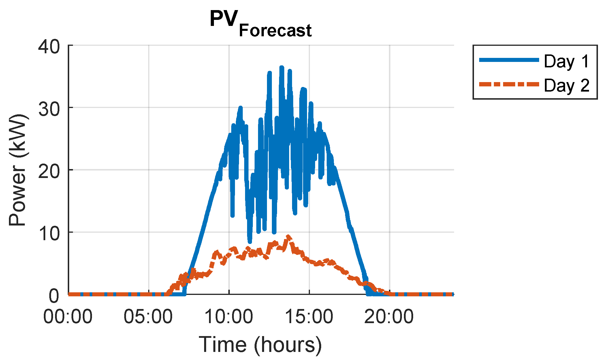
4.1. Two-Day Simulation Results

For this case, we consider PV forecast data from an actual site for a two-day period [3], one day with high solar variability and one day that is overcast, with requested power and building load profiles also provided for both days. The available solar forecast data along with requested power and building loads are provided to the MPC algorithm and the results for building load and energy storage operations are obtained. Figure 5 shows the forecasted PV from an actual PV array for the two day period. We can see the high variability in the first day and low PV power in the second day. The PV forecast variability in the first day may cause issues with maintaining the ramp rate constraint while the reduced level of PV power availability on the second day requires assistance from the energy storage unit to meet the requested power requirements. The maximum generated power from the PV array is 50 kW, the maximum energy storage unit capacity is 200 kWh, the charge/discharge limit of the battery is 50 kW and 50 kVar for real and reactive power, and the usable range for SoC is between 5% and 95%. For the MPC algorithm, the length of the prediction and control horizons in minutes are: $N_{p,BL}=15,N_{c,BL}=5,N_{p,ES}=5$, and $N_{c,ES}=1$.

The real and reactive requested power setpoints provided by the system controller and the measured building load are shown in Figure 6, respectively. We can see that in general the building is consuming more power than the requested power. Therefore, the energy storage unit will need to compensate for this difference. The controllable loads range from $-15\mathrm{kW}$ to $15\mathrm{kW}$ for real power and $-5\mathrm{kVar}$ to $5\mathrm{kVar}$ for reactive power.

4.1.1. Day 1 Simulation Results

The MPC algorithm is applied to the data from the first day and the results for real power are given in Figure 7. The original data before applying our proposed MPC algorithm is shown in Figure 7a, where we can see the difference between the requested power setpoint from the system controller and the original aggregated power from the building load and PV. Figure 7b shows the system’s response to the MPC1 algorithm, and we can see a shift in total power that makes it closer to the requested power. The shift provided by the controllable building loads are calculated by the MPC1 algorithm. Although the resulted aggregated power is improved, there are still fluctuations that violate the ramp rate constraint. As shown in Figure 7c, the fluctuations are reduced by using the energy storage unit controlled by the MPC2 algorithm. We can see that the system tracks the requested power very well, except at some points such as around 06:00 in the morning. At this time, the building starts consuming more power as the day starts while the requested power stays the same. Therefore, additional power needs to be generated by both the PV and the energy storage units. The PV generates zero power due to the lack of sunlight at this time of day, so the energy storage must provide the necessary power within its operating constraints to compensate for the difference. The operating constraints limit the amount of power that can be delivered by the energy storage, and results in some spikes in the total power. The ramp rate and energy storage SoC constraints are both met as shown in Figure 7d,e, respectively. Based on the energy storage SoC at midnight and the day-ahead forecasted values for building load and PV generation provided to the system controller at midnight, the initial SoC for day 2 is also calculated to be 73.55% as shown in Figure 8.

The reactive power results are shown in Figure 9. Similar to the real power results, we can see how $\Delta BL$ in MPC1 and energy storage in MPC2 have improved the trajectory tracking response while maintaining the ramp rate requirement. It should be noted that the spikes that are present during the early morning hours cannot be improved by the battery due to its ramp rate constraint.

4.1.2. Day 2 Simulation Results

The MPC algorithm is applied to the Day 2 data, with initial SoC of 27.87% that is the battery SoC at midnight (end of the previous day). The system halts all MPC2 calculations to let the battery charge until it reaches the desired SoC of 73.55% determined by the overnight calculations at the end of Day 1. The requested power and building load profiles for Day 2 are similar to Day 1, and all other constraints are also the same. The results of MPC1, MPC2 and the constraints for real power are shown in Figure 10. We can see that the requested power is met, while all the constraints are satisfied. The sudden peak in the ramp rate constraint at 2:00 a.m. is when the battery has reached its desired SoC and the system resumes MPC2 calculations. Similarly, the reactive power response of the system is also shown in Figure 11 that further verifies the performance of the proposed algorithm.

4.2. System Operational Changes Simulation Results

For this case, we consider scenarios where there are sudden changes in the requested power setpoints from the system controller, building load consumption and generated PV. The proposed algorithm is evaluated for these scenarios to observe its performance in overcoming the difficulties that may occur during actual system operation at Case Western Reserve University.

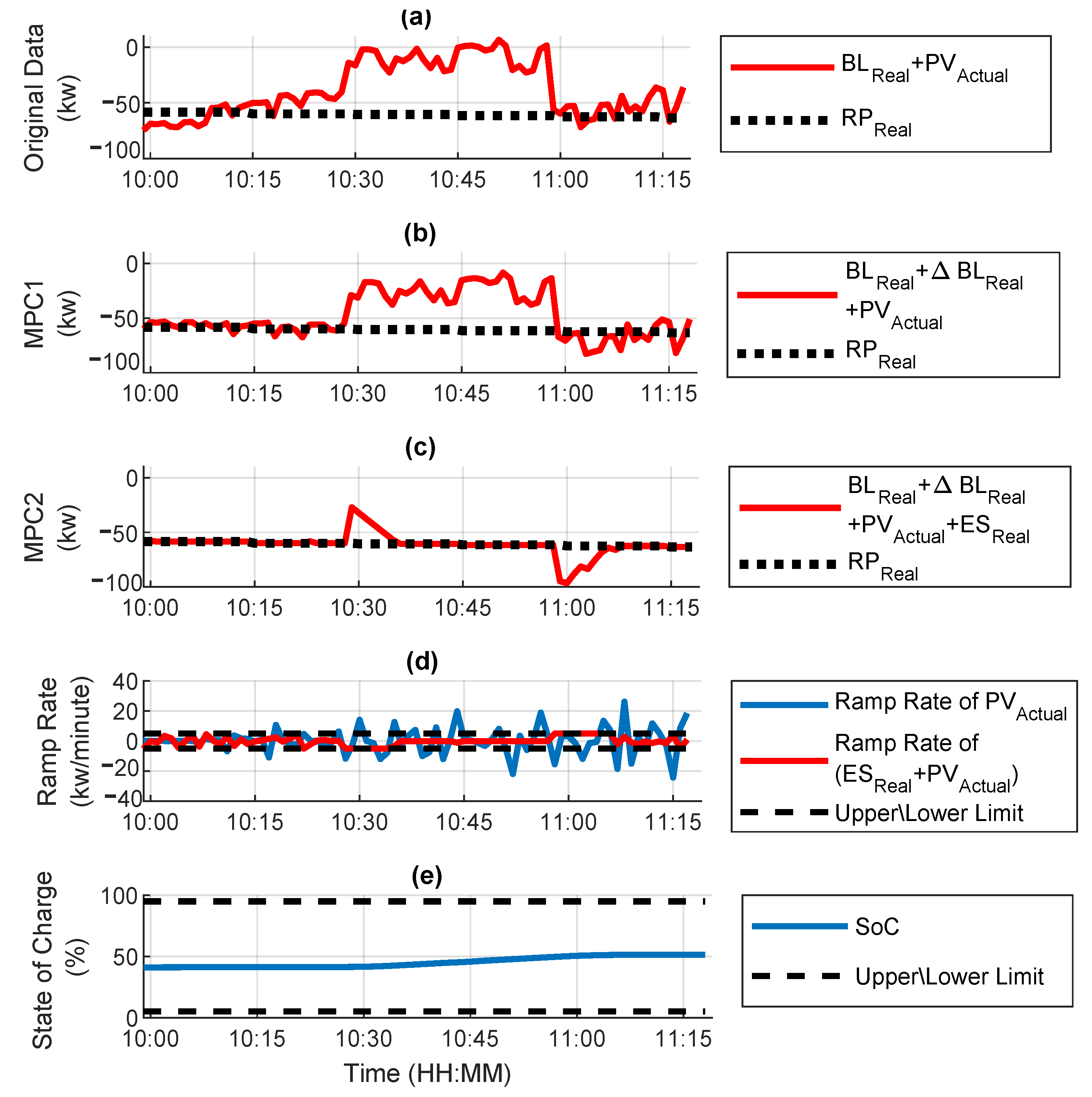
4.2.1. Scenario 1-Increased Requested Power Consumption

In this scenario, the real requested power consumption setpoint from the system controller is increased to 100 kW at 10:30 in the morning for half an hour. As the building load consumption and generated PV do not change, the requested increase in power consumption should be compensated for by $\Delta BL$ and energy storage as shown in Figure 12. We can see that prior to the increase, $\Delta BL$ was at its limit of $-15$ kW and cannot further improve the total power consumption from the building. The higher power consumption must then be compensated for by the battery and we can see the increase in $E{S}_{\mathrm{Real}}$ from 10:30 to 11:00 a.m. Figure 13 shows the performance of the algorithm for this scenario and we can see that the updated requested power setpoint is achieved by the system while satisfying the operational limits. Note that around 10:30 and 11:30 a.m., when the setpoint is suddenly changed, the overall power consumption does not meet the requested setpoint. In this case, the battery cannot compensate for this change due to its ramp rate constraint.

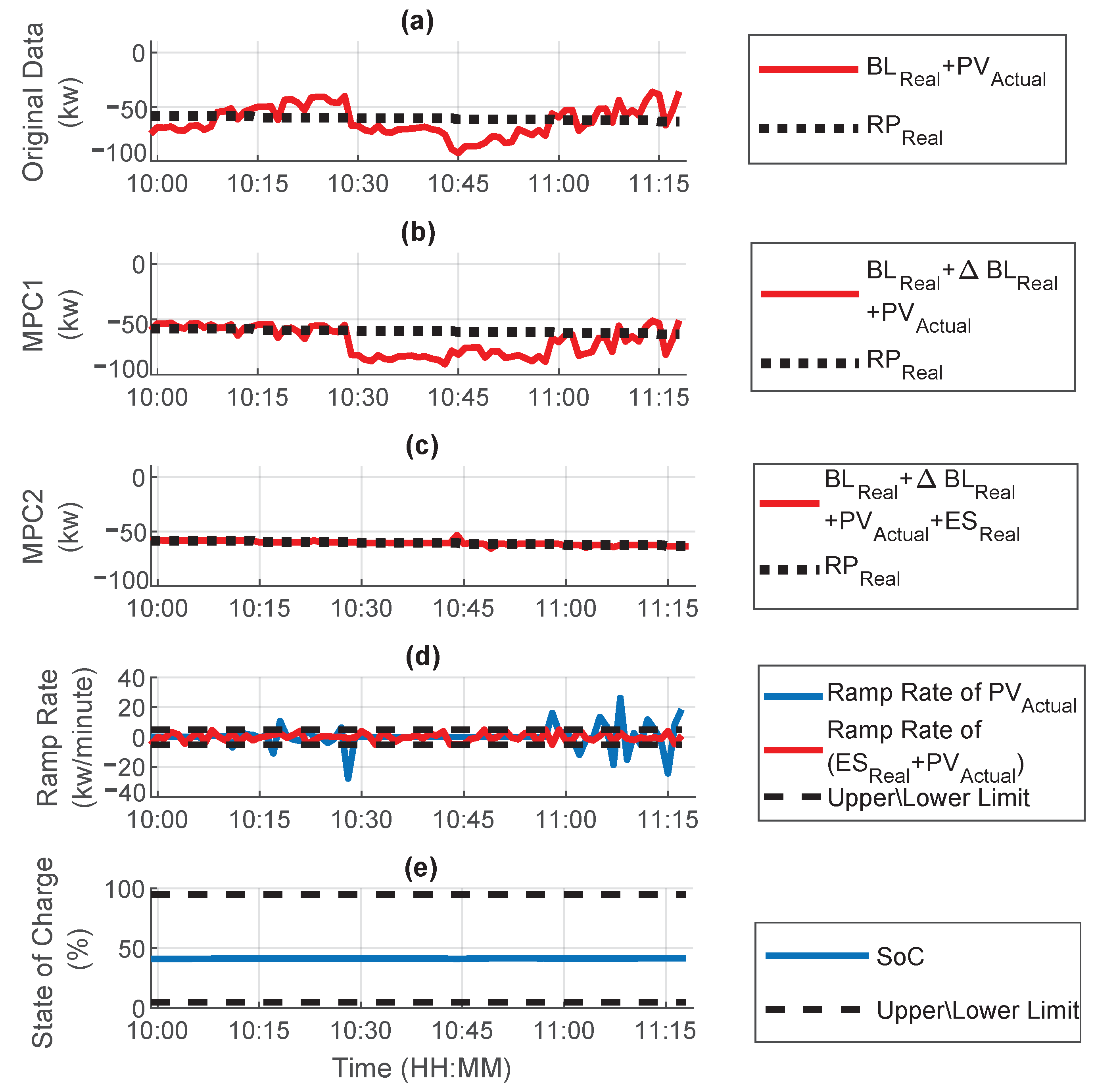
4.2.2. Scenario 2-Decreased Building Load Consumption

Similar to Scenario 1 in Section 4.2.1, the building load consumption is decreased at 10:30 a.m. for half an hour. With the decrease in the building load consumption, while the overall power consumption is not changed, the battery should compensate for this change by consuming more power, which can be observed in Figure 14. The results in Figure 15 confirm the performance of the proposed algorithm in maintaining the requested power setpoints from the system controller during the sudden decrease in requested building load consumption from the system controller.

4.2.3. Scenario 3-Loss of Generated Power from PV

In this scenario, we consider the case where there is a loss of PV power generation for half an hour during the day. This loss may happen due to failures in the PV generation unit or weather conditions. This sudden change was not expected and is not reflected in the forecasted PV provided to the algorithm, but it will be resolved by the ES trim block. As we can see in Figure 16, the un-trimmed $E{S}_{\mathrm{Real}}$ has not considered the actual loss in PV generated power because it is calculated based on the forecasted PV, not actual PV. However, we can see that the PV loss is considered in the trimmed $E{S}_{\mathrm{Real}}$ that shows an increase in power supplied by the battery during the period of PV generation loss. Figure 17 confirms the performance of the proposed algorithm in tracking the system controller setpoints during the period of sudden PV generation loss.

5. Conclusions

This paper has developed a two-level algorithm that dynamically adjusts real/reactive building load power in coordination with real/reactive energy storage power to constrain the ramping rate from solar intermittency and to manage overall real/reactive building load power based on requests from the system controller and electrical distribution network operators. The local controller receives requested power setpoints from the system controller, and the requested power trajectory can be defined to achieve numerous operational objectives of system performance such as energy efficiency, grid optimization, etc. The control algorithm is based on the Model Predictive Control (MPC) framework and uses PV forecast data and constraints on operating variables such as PV ramp rate, building loads, and energy storage SoC in the algorithm, and also addresses errors in the PV forecast using an ES trim to adjust the output of the energy storage system accordingly. It calculates the next day initial SoC based on PV forecast, and predicted requested power and building load for the next day. The mathematical formulation of the problem was presented and details of the algorithm were provided. Simulation studies are conducted to evaluate the performance of the local control system (MPC1 and MPC2) before actual deployment on the CWRU campus. Two continuous sample days with different PV forecasts from an operating PV power plant are considered, and the algorithm was used to adjust building loads and charging and discharging of energy storage to meet the overall requested power and operating constraints. The algorithm’s performance in the case of sudden changes in the electrical distribution system (system controller) requests, building load consumption and loss of PV generation were also evaluated. Based on the performance analysis as summarized in this paper, the system developed was deployed on a building on the CWRU campus. The design, deployment and testing of the system and local (MPC) controllers on the CWRU campus will be described in detail in a subsequent publication.

References

1. Jewell, W.; Ramakumar, R. The Effects of Moving Clouds on Electric Utilities with Dispersed Photovoltaic Generation. IEEE Trans. Energy Convers. 1987, EC-2, 570–576. [Google Scholar] [CrossRef]
2. Kern, E.C.; Gulachenski, E.M.; Kern, G.A. Cloud effects on distributed photovoltaic generation: Slow transients at the Gardner, Massachusetts photovoltaic experiment. IEEE Trans. Energy Convers. 1989, 4, 184–190. [Google Scholar] [CrossRef]
3. Trueblood, C.; Coley, S.; Key, T.; Rogers, L.; Ellis, A.; Hansen, C.; Philpot, E. PV Measures Up for Fleet Duty: Data from a Tennessee Plant Are Used to Illustrate Metrics That Characterize Plant Performance. IEEE Power Energy Mag. 2013, 11, 33–44. [Google Scholar] [CrossRef]
4. Kakimoto, N.; Satoh, H.; Takayama, S.; Nakamura, K. Ramp-Rate Control of Photovoltaic Generator With Electric Double-Layer Capacitor. IEEE Trans. Energy Convers. 2009, 24, 456–473. [Google Scholar] [CrossRef]
5. Tam, K.S.; Kumar, P.; Foreman, M. Enhancing the utilization of photovoltaic power generation by superconductive magnetic energy storage. IEEE Trans. Energy Convers. 1989, 4, 314–321. [Google Scholar] [CrossRef]
6. Hund, T.D.; Gonzalez, S.; Barrett, K. Grid-Tied PV system energy smoothing. In Proceedings of the 35th IEEE Photovoltaic Specialists Conference, Honolulu, HI, USA, 20–25 June 2010. [Google Scholar]
7. Li, X.; Hui, D.; Lai, X. Battery Energy Storage Station (BESS)-Based Smoothing Control of Photovoltaic (PV) and Wind Power Generation Fluctuations. IEEE Trans. Sustain. Energy 2013, 4, 464–473. [Google Scholar] [CrossRef]
8. Ellis, A.; Schoenwald, D.; Hawkins, J.; Willard, S.; Arellano, B. PV output smoothing with energy storage. In Proceedings of the 38th IEEE Photovoltaic Specialists Conference, Austin, TX, USA, 3–8 June 2012. [Google Scholar]
9. Alam, M.J.E.; Muttaqi, K.M.; Sutanto, D. A Novel Approach for Ramp-Rate Control of Solar PV Using Energy Storage to Mitigate Output Fluctuations Caused by Cloud Passing. IEEE Trans. Energy Convers. 2014, 29, 507–518. [Google Scholar]
10. Salehi, V.; Radibratovic, B. Ramp rate control of photovoltaic power plant output using energy storage devices. In Proceedings of the 2014 IEEE PES General Meeting | Conference & Exposition, National Harbor, MD, USA, 27–31 July 2014; pp. 1–5. [Google Scholar]
11. Pascual, J.; Arcos-Aviles, D.; Ursúa, A.; Sanchis, P.; Marroyo, L. Energy management for an electro-thermal renewable–based residential microgrid with energy balance forecasting and demand side management. Appl. Energy 2021, 295, 117062. [Google Scholar] [CrossRef]
12. Godina, R.; Rodrigues, E.M.G.; Shafie-khah, M.; Pouresmaeil, E.; Catalão, J.P.S. Energy optimization strategy with Model Predictive Control and demand response. In Proceedings of the 2017 IEEE International Conference on Environment and Electrical Engineering and 2017 IEEE Industrial and Commercial Power Systems Europe (EEEIC/I CPS Europe), Milan, Italy, 6–9 June 2017; pp. 1–5. [Google Scholar]
13. Ospina, J.; Harper, M.; Newaz, A.; Faruque, M.O.; Collins, E.G.; Meeker, R.; Ainsworth, N. Optimal Energy Management of Microgrids using Sampling-Based Model Predictive Control Considering PV Generation Forecast and Real-time Pricing. In Proceedings of the 2019 IEEE Power Energy Society General Meeting (PESGM), Atlanta, GA, USA, 4–8 August 2019; pp. 1–5. [Google Scholar] [CrossRef]
14. Alarcón, M.A.; Alarcón, R.G.; González, A.H.; Ferramosca, A. Economic model predictive control for energy management in a hybrid storage microgrid. In Proceedings of the 2021 XIX Workshop on Information Processing and Control (RPIC), San Juan, Argentina, 3–5 November 2021; pp. 1–6. [Google Scholar] [CrossRef]
15. Razmara, M.; Bharati, G.R.; Hanover, D.; Shahbakhti, M.; Paudyal, S.; Robinett, R.D. Enabling Demand Response programs via Predictive Control of Building-to-Grid systems integrated with PV Panels and Energy Storage Systems. In Proceedings of the 2017 American Control Conference (ACC), Seattle, WA, USA, 24–26 May 2017; pp. 56–61. [Google Scholar] [CrossRef]
16. Farrokhifar, M.; Bahmani, H.; Faridpak, B.; Safari, A.; Pozo, D.; Aiello, M. Model predictive control for demand side management in buildings: A survey. Sustain. Cities Soc. 2021, 75, 103381. [Google Scholar] [CrossRef]
17. Eseye, A.T.; Knueven, B.; Vaidhynathan, D.; King, J. Scalable Predictive Control and Optimization for Grid Integration of Large-Scale Distributed Energy Resources: Preprint; National Renewable Energy Lab. (NREL): Golden, CO, USA, 2022. [Google Scholar]
18. Mahfuz-Ur-Rahman, A.M.; Islam, M.R.; Muttaqi, K.M.; Sutanto, D. An Effective Energy Management With Advanced Converter and Control for a PV-Battery Storage Based Microgrid to Improve Energy Resiliency. IEEE Trans. Ind. Appl. 2021, 57, 6659–6668. [Google Scholar] [CrossRef]
19. Joe Qina, S.; Badgwell, T.A. A survey of industrial model predictive control technology. Control Eng. Pract. 2003, 11, 733–764. [Google Scholar] [CrossRef]
20. Doostmohammadi, F.; Esmaili, A.; Sadeghi, S.H.H.; Nasiri, A.; Talebi, H.A. A model predictive method for efficient power ramp rate control of wind turbines. In Proceedings of the IECON 2012—38th Annual Conference on IEEE Industrial Electronics Society, Montreal, QC, Canada, 25–28 October 2012. [Google Scholar]
21. You, S.; Liu, Z.; Zong, Y. Model predictive control for power fluctuation supression in hybrid wind/PV/battery. In Proceedings of the 4th International Conference on Microgeneration and Related Technologies, Tokyo, Japan, 28–30 October 2015. [Google Scholar]
22. Wang, T.; Kamath, H.; Willard, S. Control and Optimization of Grid-Tied Photovoltaic Storage Systems Using Model Predictive Control. IEEE Trans. Smart Grid 2014, 5, 1010–1017. [Google Scholar] [CrossRef]
23. Raoufat, E.; Asghari, B.; Sharma, R. Model Predictive BESS Control for Demand Charge Management and PV-Utilization Improvement. In Proceedings of the IEEE Power & Energy Society Innovative Smart Grid Technologies Conference (ISGT), Washington, DC, USA, 19–22 February 2018. [Google Scholar]
24. Parisio, A.; Rikos, E.; Glielmo, L. A Model Predictive Control Approach to Microgrid Operation Optimization. IEEE Trans. Control Syst. Technol. 2014, 22, 1813–1827. [Google Scholar] [CrossRef]
25. Mayne, D.Q.; Rawlings, J.B.; Rao, C.V.; Scokaert, P.O.M. Constrained model predictive control: Stability and optimality. Automatica 2000, 36, 789–814. [Google Scholar] [CrossRef]
26. Boyd, S.; Vandenberghe, L. Convex Optimization; Cambridge University Press: Cambridge, UK, 2009. [Google Scholar]
27. Razmara, M.; Bharati, G.R.; Shahbakhti, M.; Paudyal, S.; Robinett, R.D. Bilevel Optimization Framework for Smart Building-to-Grid Systems. IEEE Trans. Smart Grid 2018, 9, 582–593. [Google Scholar] [CrossRef]
28. Picasso, B.; Vito, D.; Scattolini, R.; Colaneri, P. An MPC approach to the design of two-layer hierarchical control systems. Automatica 2010, 46, 823–831. [Google Scholar] [CrossRef]
29. Kathirgamanathan, A.; De Rosa, M.; Mangina, E.; Finn, D.P. Data-driven predictive control for unlocking building energy flexibility: A review. Renew. Sustain. Energy Rev. 2021, 135, 110120. [Google Scholar] [CrossRef]
Figure 1. System schematic.
Energies 15 03521 g001
Figure 2. Receding horizons in the MPC algorithm.
Energies 15 03521 g002
Figure 3. MPC local control structure.
Energies 15 03521 g003
Figure 4. Real-time actual and forecast PV.
Energies 15 03521 g004
Figure 5. PV forecast comparison.
Energies 15 03521 g005
Figure 6. Requested power and building load comparison for (a) real power and (b) reactive power.
Energies 15 03521 g006
Figure 7. Day 1 real power (a) original data, (b) MPC1 simulation result, (c) MPC2 simulation results, (d) ramp rate constraint, and (e) energy storage SoC constraint.
Energies 15 03521 g007
Figure 8. Day 2 initial SoC calculation.
Energies 15 03521 g008
Figure 9. Day 1 reactive power (a) original data, (b) MPC1 simulation result, (c) MPC2 simulation results, and (d) ramp rate constraint.
Energies 15 03521 g009
Figure 10. Day 2 real power (a) original data, (b) MPC1 simulation result, (c) MPC2 simulation results, (d) ramp rate constraint, and (e) energy storage SoC constraint.
Energies 15 03521 g010
Figure 11. Day 2 reactive power (a) original data, (b) MPC1 simulation result, (c) MPC2 simulation results, and (d) ramp rate constraint.
Energies 15 03521 g011
Figure 12. Scenario 1—battery and building load performance.
Energies 15 03521 g012
Figure 13. Scenario 1—algorithm performance for real power (a) original data, (b) MPC1 simulation result, (c) MPC2 simulation results, (d) ramp rate constraint, and (e) energy storage SoC constraint.
Energies 15 03521 g013
Figure 14. Scenario 2—battery and building load performance.
Energies 15 03521 g014
Figure 15. Scenario 2—algorithm performance for real power (a) original data, (b) MPC1 simulation result, (c) MPC2 simulation results, (d) ramp rate constraint, and (e) energy storage SoC constraint.
Energies 15 03521 g015
Figure 16. Scenario 3—battery and building load performance.
Energies 15 03521 g016
Figure 17. Scenario 3—algorithm performance for real power (a) original data, (b) MPC1 simulation result, (c) MPC2 simulation results, (d) ramp rate constraint, and (e) energy storage SoC constraint.
Energies 15 03521 g017
Publisher’s Note: MDPI stays neutral with regard to jurisdictional claims in published maps and institutional affiliations.