Article

Characteristic Forced and Spontaneous Imbibition Behavior in Strongly Water-Wet Sandstones Based on Experiments and Simulation

by
Pål Østebø Andersen
1,*,
Liva Salomonsen
1 and
Dagfinn Søndenaa Sleveland
2
1
Department of Energy Resources, Faculty of Science and Technology, University of Stavanger, 4021 Stavanger, Norway
2
Department of Energy and Petroleum Engineering, Faculty of Science and Technology, University of Stavanger, 4021 Stavanger, Norway
*
Author to whom correspondence should be addressed.
Energies 2022, 15(10), 3531; https://doi.org/10.3390/en15103531
Submission received: 24 March 2022 / Revised: 9 May 2022 / Accepted: 10 May 2022 / Published: 11 May 2022
(This article belongs to the Special Issue Management of High Water Cut and Mature Petroleum Reservoirs)

Abstract

:
Forced and spontaneous imbibition of water is performed to displace oil from strongly water-wet Gray Berea (~130 mD) and Bentheimer (~1900 mD) sandstone core plugs. Two nonpolar oils (n-heptane and Marcol-82) were used as a non-wetting phase, with viscosities between 0.4 and 32 cP and brine (1 M NaCl) for the wetting phase with viscosity 1.1 cP. Recovery was measured for both imbibition modes, and pressure drop was measured during forced imbibition. Five forced imbibition tests were performed using low or high injection rates, using low or high oil viscosity. Seventeen spontaneous imbibition experiments were performed at four different oil viscosities. By varying the oil viscosity, the injection rate and imbibition modes, capillary and advective forces were allowed to dominate, giving trends that could be captured with modeling. Full numerical simulations matched the experimental observations consistently. The findings of this study provide better understanding of pressure and recovery behavior in strongly water-wet systems. A strong positive capillary pressure and a favorable mobility ratio resulting from low water relative permeability were main features explaining the observations. Complete oil recovery was achieved at water breakthrough during forced imbibition for low and high oil viscosity and the recovery curves were identical when plotted against the injected volume. Analytical solutions for forced imbibition indicate that the pressure drop changes linearly with time when capillary pressure is negligible. Positive capillary forces assist water imbibition, reducing the pressure drop needed to inject water, but yielding a jump in pressure drop when the front reaches the outlet. At a high injection rate, capillary forces are repressed and the linear trend between the end points was clearer than at a low rate for the experimental data. Increasing the oil viscosity by a factor of 80 only increased the spontaneous imbibition time scale by five, consistent with low water mobility constraining the imbibition rate. The time scale was predicted to be more sensitive to changes in water viscosity. At a higher oil-to-water mobility ratio, a higher part of the total recovery follows the square root of time. Our findings indicate that piston-like displacement of oil by water is a reasonable approximation for forced and spontaneous imbibition, unless the oil has a much higher viscosity than the water.

1. Introduction

In this work we are interested in how imbibition takes place in strongly wetted porous media, i.e., we study processes where a wetting phase (water) displaces a non-wetting phase (oil), with focus on oil recovery applications. Imbibition multiphase flow processes in porous media have more general applications within subsurface energy storage and production (geothermal, petroleum, hydrogen) and geological storage of carbon dioxide [1,2].
Core plug experiments are routinely performed to measure how water can displace oil (referred to as imbibition), mimicking the water flooding process at reservoir scale. The cores are saturated with initial saturations of oil and water and aged to allow the system to be equilibrated with the intention that a representative wetting state is obtained. Outcrop core samples are often studied as they are cheap, available and have repeatable behavior. As they have not stored hydrocarbons geologically, they are strongly water-wet (SWW), although aging with polar oils can modify their wetting state. Reservoir rocks, which have stored polar oils over geological time are usually not SWW and their wettability must be measured [3]. Depending on which boundary conditions are applied, there are several mechanisms that can assist or resist the imbibition.
During forced imbibition, water is injected through the core at a specified rate or pressure drop. If the rates are high, the advective forces can be assumed dominant and the measurements of pressure drop and fluid production can be applied to calculate relative permeability [4,5,6] and residual oil saturation. Generally, significant capillary diffusion can smear the saturation front and lead to wetting phase accumulation at the outlet where the capillary pressure is zero [7,8]. Rapoport and Leas [9] showed that the relative importance of capillary diffusion reduced with a higher product of core length, water viscosity and injection rate. In their experiments the water breakthrough recovery varied with these parameters until the product had exceeded a critical limit. Gupta and Maloney [10] and Andersen [11] presented intercept methods to correct relative permeability for capillary end effects, especially relevant for estimating the end point water relative permeability and residual oil saturation during water flooding. Positive capillary pressure is obtained at all mobile saturations in SWW media [1,12] and leads to water advancing into the system during imbibition. However, it also traps water and resists it from leaving the core during flooding, meaning a delayed breakthrough can be observed. Craig [13] and Anderson [14] associated water flooding of SWW media with linear recovery, meaning that most of the mobile oil was recovered before significant water production occurred. Less water-wet media had earlier water-breakthrough. In SWW media, water flows as films on the rock surfaces while the oil flows centrally in the pores and is eventually trapped as isolated droplets that the water flows around. Macroscopically low water relative permeability and comparatively high oil relative permeability are thus observed for SWW media [15,16,17]. Yortsos and Fokas [18] presented exact solutions for water flooding an SWW system at constant rate accounting for capillary forces, but considered a semi-infinite system, and thus did not account for outlet boundary effects. Their simulations demonstrated rapid water progress at strong capillary forces and early water breakthrough. The latter may not be valid since blockage was not accounted for, nor is it observed experimentally. Odeh and Dotson [19] found that relative permeability data from dynamic experiments could be corrected based on identifying lines through unaffected data.
Spontaneous imbibition (SI) is the second main mode of imbibition. In that case a core is exposed to wetting fluid (water) to allow spontaneous uptake by capillary forces and the simultaneous displacement of non-wetting fluid [20]. This is relevant in naturally fractured reservoirs where oil in disconnected matrix blocks is not displaced advectively. If all the core faces are open (AFO) and exposed to water, the traditional Amott test [21] is considered. In many cases some of the surfaces are sealed to make the flow entirely linear or radial. As long as the system is symmetric, the flow of oil and water will be counter-current. Gravity may cause more oil production at the top than at the bottom or trap some oil if the top side is closed. A different setup for SI is exposing parts of the core to the wetting phase and other parts to the nonwetting phase. In that case water enters at the former side and oil is produced predominantly at the latter side and to a lesser extent at the water exposed side [17,22,23,24]. The flow is said to be co-current. This setup is considered more complex to perform and interpret than counter-current imbibition and can result in highly varying recovery profiles with time and relative amounts of co- and counter-current production depending on mobility ratio, capillary back pressure, wettability and viscous coupling effects [25,26,27]. It is however relevant since matrix blocks are gradually submerged during waterflooding and thus undergo an early stage of recovery in co-current mode.
Counter-current SI has been investigated thoroughly to understand the impact of fluid-rock parameters, wettability, geometry, flow mechanisms etc., with the intention of accurate upscaling to reservoir matrix block scales [28,29,30,31,32]. An important feature of SWW media is that SI can yield as high a recovery as forced imbibition, while in more oil-wet media SI yields, it yields a lower recovery than forced imbibition [33]. Scaling relations accounting for changes in the stated parameters have been developed, where we note that Ma et al. [29] suggested an effective length to convert arbitrary boundary conditions (closed or open to water) and geometries to a 1D linear system with one side open and the other closed. Their time scale included other a priori parameters such as permeability, viscosities, porosity and interfacial tension. The time scale in general, however depends on the capillary diffusion coefficient function, which changes in a complex way with variation in viscosities and wettability [34]. This function or its constituents are typically unknown. Several works have attempted to improve scaling for a given rock system (usually SWW) by modifications of Ma et al.’s time scale with viscosity coefficients, e.g., [31,35,36]. Zhou et al. [37] evaluated the mobility in the diffusion coefficient at their end points. McWhorter and Sunada [34] showed that 1D linear counter-current SI has a recovery profile proportional with the square root of time, regardless of saturation functions and other input. That is however valid only until the no-flow boundary is encountered. Their solution was expressed implicitly with integral functions but could be used for scaling data where all input parameters were known [38,39]. Works making specific assumptions on the saturation profile (polynomial shape or piston-like displacement) and saturation functions produced more explicit but less general solutions, also with square root of time recovery profiles [40,41]. At a later time, the imbibition rate will reduce towards zero, as recovery is bounded. Note also that AFO systems, mainly applied in Amott tests are not 1D linear and may deviate from the expected linear behavior also at early time.
In this work, experiments and modeling are performed to evaluate characteristic imbibition behavior at different conditions. Outcrop sandstone with moderate and high permeability (~150 and ~2000 mD) are used together with brine and different nonpolar oils, the latter with viscosity ranging from 0.4 to 32 cP. SWW conditions are expected. All-Faces-Open Spontaneous imbibition (Figure 1 left) is performed in Amott cells to evaluate the role of oil viscosity on recovery profiles and time scales. Forced imbibition (Figure 1 right) is performed with different injection rates and viscosities to assess the role of mobility ratio and relative magnitudes of viscous to capillary forces on recovery and pressure profiles. The data are interpreted consistently using numerical simulation, scaling and simplified analytical solutions. Features are derived to interpret experimental data, which may indicate the presence of strong capillary forces during flooding or the relative dominance of one phase’s mobility compared to the other.
In comparison, previous works have investigated the impact of viscosity on imbibition, but interpreted this independent of flooding experiments and mainly used simple scaling laws without investigating whether the data can be explained consistently with full saturation functions. We are interested in whether the features observed in spontaneous and forced imbibition for SWW media have a consistent explanation rooted in the saturation functions and whether other trends can be predicted as a result. For example, we wish to investigate:
-
Why is most of or all the mobile oil recovered before water breakthrough when flooding SWW media?
-
Do end effects prevent water breakthrough significantly or is the displacement piston-like?
-
Can capillary forces be detected from the pressure drop profile during flooding?
-
How does a change in oil viscosity affect time scale and recovery profile during spontaneous imbibition? What if we change water viscosity instead?

2. Experimental Setup

2.1. Fluids

The oils used were n-Heptane and Marcol 82 and mixtures of them to give intermediate viscosities. The brines used were 0.1 M NaCl and 1 M NaCl, filtered using a vacuum pump and a 0.65 μm filter. Interfacial tension (IFT) between oil and 1 M NaCl was measured using a tensiometer and platinum ring. An overview of oil and brine properties is shown in Table 1. The experiments were performed at room temperature ~20 °C. Methanol and toluene were used for core cleaning.

2.2. Rock Material and Core Preparation

Core material was collected from Grey Berea sandstone, formed during the Late Devonian and quarried from Ohio, USA [42]; and Bentheimer sandstone deposited during the Lower Cretaceous and sourced from a quarry near the Dutch–German border [43]. Both formations have subsurface accumulations of oil and gas. These sandstones provide permeability from a few 100 mD to a few D. The mineralogical composition for both these rocks was reported semi-quantitatively to 94 wt% quartz, 1 wt% kaolinite, 1 wt% muscovite and 1 wt% microline [44,45]. Cores originally ~20 cm long (named with letters) were cut in three equal parts using a Stuers Discotom 5 saw. The cores were then ground at both ends using a GCTS Testing Systems RSG-075 2-in-1 Specimen Grinder and Saw to render the end faces flat and perpendicular. The smaller plugs were numbered 1–3 accordingly. A core plug from each formation are shown in Figure 2. Cores that were damaged or used for training are not included in the following.
Basic core measurements are listed in Table 2. Length L and diameter D values were obtained with caliper and used to find the bulk volume V b . The matrix volume V m was measured with the Vinci PoroPerm device. Pore volume at unconfined stress was calculated by their difference and the (unconfined) porosity by the ratio of pore volume to bulk volume. Measurements were also made of pore volume and gas permeability for each core at a net confining pressure of 10 bar. The reduction in pore volume by confining stress was 2–3% and we assumed the permeability measured at confined pressure (as during forced imbibition) was also representative for unconfined conditions (as during spontaneous imbibition). The gas permeability values were obtained at an atmospheric outlet pressure, and not corrected for Klinkenberg effects, meaning the values may be a little higher than the corresponding liquid permeability. This has little consequence as the end point liquid permeability values were measured, making the gas permeability just a reference value.

2.3. Establishing Initial Conditions

To establish initial water saturation, a clean and dry core sample was saturated using 0.1 mol/L NaCl and then drained to a specified water saturation of 10% by water evaporation in a vacuum desiccator. The initial brine concentration gave the brine a concentration of 1.0 mol/L when the target saturation was reached. Next, the cores were saturated with oil, which in this study was either n-Heptane, Marcol 82 or a mixture of them. The core was then ready for either forced or spontaneous imbibition.

2.4. Flooding Rig Equipment

A Quizix QX pump from Ametek Chandler Engineering was used in the flooding rig. The core sample was mounted in a core holder of Hassler type. As the experiment started, the differential pressure, back pressure and overburden pressure were measured continuously by Rosemount 3051TM CoplanarTM Pressure Transmitters. The measurement range for differential pressure measurements was 0–62 mbar for the low range transmitter, and 0–2400 mbar for the high range transmitter. Management of the pump and datalogging was performed from a computer using the dedicated pump software PumpWorks, which was supplied by Ametek to control the QX-pumps.

2.5. Measurement of End Point Permeabilities

The effective oil permeability was measured at initial water saturation k o ( s w i ) , after establishing initial conditions, before performing either forced or spontaneous imbibition. The flooding rig was prepared by saturating all tubings with the relevant oil. The core sample was then placed in the core holder and put under 12 bar confining pressure and a back pressure of 2 bar. The pressure drop was measured at four different rates, then linear regression and Darcy’s law were used to calculate the effective oil permeability of the core sample at the initial water saturation. After the forced imbibition experiments, the effective water permeability at residual oil saturation, k w ( s o r ) , was measured using the same method, with flooding brine at four different rates. Relative permeability endpoints were calculated by dividing the calculated effective permeability by the gas permeability of the core sample.

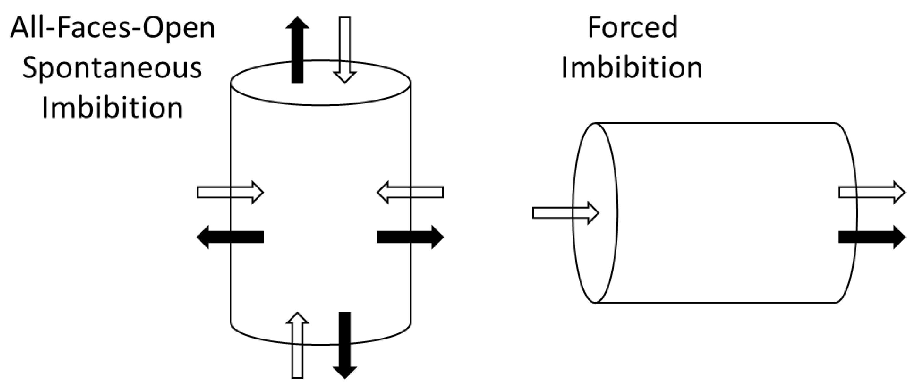
2.6. Spontaneous Imbibition Tests

All-Faces-Open spontaneous imbibition was performed using a clean and leak-proof Amott cell. A coiled steel wire was used as a shock absorber. A core saturated with oil and initial water saturation, was placed in the cell on top of the steel wire. A magnet was used to loosen oil bubbles potentially sticking to the glass. The time was started when the Amott cell was filled with imbibing fluid 1 mol/L NaCl brine. The cell was shaken regularly, and the location of the fluid meniscus was read while noting the time. When the oil production had stabilized, the experiment was ended.

2.7. Forced Imbibition

After measuring k o ( s w i ) the tubes of the rig were cleaned for oil using n-heptane and compressed air. The core was kept at 12 bar overburden pressure and a back pressure of 2 bar (10 bar net confining pressure). Five forced imbibition experiments were performed, using two oils (n-Heptane or Marcol 82) and two rates (2 mL/h or 15 mL/h). The produced oil was collected in a burette/separator. A camera was used to photograph the oil level in the burette/separator at a specified frequency. The pressure drop from inlet to outlet of the core was recorded continuously.

2.8. Procedure for Cleaning Cores Using Soxhlet Extractor

The core samples were cleaned of oil, water and salts using a Soxhlet extractor. Toluene was used to remove oils from the sample while methanol was used to remove water and salts.

3. Theory

3.1. General Description of 1D Two-Phase Flow

Oil-water 1D linear flow in porous media is considered with incompressible rock and fluids, and the fluids are immiscible. The fluid saturations s i and pressures p i are related by volume and capillary pressure constraints:
s o + s w = 1 ,     p o p w = P c ( s w )
The system can be described by a water transport equation and a pressure equation:
ϕ t s w = x ( u T f w + K λ o f w x P c ) ,
x ( λ o x P c + λ T x p w ) = 0
In a given experiment we assume porosity ϕ , absolute permeability K , fluid viscosities μ i are constant and that relative permeabilities k r i and capillary pressure P c are functions of water saturation s w . Fluid mobilities λ i are defined by the ratio of relative permeability k r i and viscosity μ i , while the fractional flow function f w is the water mobility divided by the total mobility λ T .
λ i = k r i μ i ,     P c ( s w ) = σ o w ϕ / K J ( s w ) ,     f w = λ w λ T ,     λ T = λ o + λ w
As a base assumption for interpreting all the experiments, the relative permeability k r i and scaled capillary pressure J ( s w ) are assumed to be the same. That is reasonable since we use same brine and initial saturation, artificial oils without polar components and outcrop sandstone samples, such that similar wetting states (strong water-wetness) can be expected. Although counter-current flow can yield lower effective relative permeability than during co-current flow [17,46] we will assume such effects are negligible. Oil recovery R F is reported as the fraction of mobile oil produced:
R F = s ¯ w s w r Δ s w = S ¯ ,     S = s w s w r Δ s w ,     Δ s w = 1 s o r s w r
As noted, recovery equals the (spatial) average of normalized water saturation S , which goes from zero to one when the water saturation varies from s w r to 1 s o r ( s i r indicates residual saturation).

3.2. Forced Imbibition

A core with length L is injected with water at x = 0 , while water and oil are produced at the outlet x = L , where the capillary pressure is zero.
u w ( x = 0 ) = u T ,     P c ( x = L ) = 0
Since u T is specified by a known injection rate, the saturation equation can be solved independently. We scale the equation with X = x L , time in mobile pore volumes T = t ( L ϕ Δ s w / u T ) , Leverett scaling, normalized saturation and a characteristic mobility λ c h = k r w * μ w to get:
T S = X ( f w ) σ λ c h K / ϕ L v T X ( λ o f w λ c h   d J d S X S ) ,
The fluid pressure drops are calculated by integrating the water pressure gradient:
Δ p w = x = 0 L [ λ o λ T x P c + u T K λ T ] d x ,     Δ p o = Δ p w + P c ( s w ( x = 0 ) )
During fluid injection the non-wetting phase pressure drop is measured, which is the highest of the two phases and corresponds to oil in a SWW system [47]. Strong capillary forces can delay the inlet saturation from reaching its maximum value (where P c = 0 ) and then the phase pressures will be different.

3.3. Counter-Current Spontaneous Imbibition

During counter-current spontaneous imbibition the length of the system can be defined by Ma et al. [29]’s characteristic length L c (adapted to a cylindrical core):
L c = V b   A i / l i = D L 2 D 2 + 2 L 2
The open boundary at x = 0 has zero capillary pressure, while the system has a no-flow boundary at x = L c . We set the outside water pressure to zero for reference:
P c ( x = 0 ) = 0 ,     p w ( x = 0 ) = 0 ,     u i ( x = L c ) = 0
Since u T = 0 at L c and u T is uniform, u T = 0 everywhere and the advective flow term can be ignored. The resulting capillary diffusion equation is solved to give saturation distributions at different times.
ϕ t s i = x ( K λ o f w x P c ) ,
The pressure distribution can be calculated based on the pressure gradient equation with zero total flux and integrating it from a known zero pressure at the open boundary:
x p w = λ o λ T x P c ,     p w ( x ) = x = 0 x λ o λ T x P c d x
The capillary diffusion equation can then be scaled using normalized saturation S , X = x / L c , T = t / τ , Leverett scaling of P c and scaling λ o f w with a characteristic mobility λ c h :
T S = τ σ λ c h L c 2 Δ s w K / ϕ X ( λ o f w λ c h d J d S X S )
The time scale is selected to make the coefficient equal to one, leaving a dimensionless, but nonlinear diffusion coefficient.
We consider three time scales based on the choice of λ c h : The first λ c h is the inverse water viscosity; the second the inverse geometric mean of the viscosities; and the third setting the end mobilities of oil and water into the expression λ o f w . These choices correspond, respectively, to the time scales of Mattax and Kyte [28], Ma et al. [29] and Zhou et al. [37], with the exception of using Ma et al.’s length L c in all cases.
τ 1 = μ w L c 2 Δ s w σ K / ϕ ,     ( λ c h = 1 μ w )
τ 2 = μ w μ o L c 2 Δ s w σ K / ϕ ,     ( λ c h = 1 μ w μ o )
τ 3 = L c 2 Δ s w σ K / ϕ ( λ o * + λ w * λ o * λ w * ) ,     ( λ c h = λ o * λ w * λ o * + λ w * )
The scales all account for variations in core shape, porosity, permeability, interfacial tension and saturation range, which appear as proportionality coefficients. The water viscosity is involved nonlinearly in the diffusion coefficient but was not varied in our experiments. Hence, τ 1 collects the data and only shows variations due to oil viscosity or possible variations in the saturation functions. Our base assumption is that k r i and J as function of S are the same for all cases. τ 2 attempts to collect viscosity variations by mean of the fluid viscosities, while τ 3 accounts for relative permeabilities and how the mobilities appear in the diffusion coefficient. As shown by McWhorter and Sunada [34], Schmid and Geiger [38] and Andersen et al. [39] a perfect scaling of viscosities and saturation functions are however only possible at an early time and depend on the entire diffusion coefficient function.
During SI, the imbibition rate declines steadily with time. In a 1D linear system, recovery is first proportional to the square root of time. At late times, the rate drops faster towards zero. Considering imbibition from all sides (and not 1D) we assume that recovery follows a more general exponent;   R F = A t α . In a log-log plot this gives a straight line log R F = log A + α log t . Data that fall on such a straight line are infinite-acting since the rate does not decline faster than in an infinite system. When the data fall below the line the infinite acting period ends. Andersen [48] found that the extent of RF in the infinite acting period (of a linear system) was directly associated with how far the capillary diffusion coefficient was shifted towards high saturations. A coefficient shifted far towards high saturations would result in almost complete recovery following a straight line against the square root of time. A shift in the coefficient towards high saturations occurs when oil gets high mobility relative to water. Andersen [48] plotted SWW data from Fischer et al. [49] and found that the data with a higher oil-to-water mobility ratio had a higher recovery in the infinite acting period, spanning 75–90% of the mobile oil.

3.4. Analytical Approximate Solutions

3.4.1. Forced Imbibition

During water injection in SWW rocks, it is commonly observed that all the mobile oil is produced before water breakthrough, with recovery being equal to the mobile pore volumes injected T m :
R F = T m ,     T m = t ( L ϕ Δ s w / u T ) ,     ( 0 < T m < 1 )
One explanation is that the mobility ratio is favorable giving associated piston-like displacement. If that is so, we can set the Darcy water velocity u w behind the front (at x f ) equal to the oil Darcy velocity u o ahead of the front:
u i = K λ w * p w f p w L x f = K λ o * p o R p o f L x f
The front capillary pressure relates the front oil and water pressures P c f = p o f p w f = P c ( s w r ) . p o f is eliminated and we solve for p w f . The expression for p w f is then substituted into the water flux equation:
p w f = λ w * ( L x f ) p w L + λ o * x f ( p o R P c ( s w r ) ) λ w * ( L x f ) + λ o * x f ,     u w = K Δ p + P c ( s w r ) L x f λ o * + x f λ w * ,
Δ p = p w L p o R is the measured pressure drop (through the oil phase) since full mobile water saturation at the inlet corresponds to zero capillary pressure ( p w L = p o L ). The Darcy velocities are constant and related to the front position as:
x f = u w ϕ Δ s w t ,     u w = u T
Apply Leverett scaling P c f = σ ϕ / K J f and solve for the pressure drop:
Δ p = u T L K ( 1 λ o * + u T t L ϕ Δ s w ( 1 λ w * 1 λ o * ) ) σ ϕ / K J ( s w r )
Divide by Δ p r e f = u T K L λ w * (the pressure drop measured if water flows at residual oil saturation) and express time in mobile pore volumes injected T m . We then obtain the following equation describing normalized pressure drop against pore volumes injected:
Δ p Δ p r e f = ( M + T m ( 1 M ) ) λ w * σ ow v T L K / ϕ J ( s w r ) ,     M = λ w * λ o * 1
The end point mobility ratio M should be less than one since we have assumed piston-like displacement, requiring the water to have a lower mobility than oil.
In case the displacement is not piston-like, we can approximate it to follow a Buckley–Leverett profile, where the capillary diffusion term does not affect the profile shape. Using similar assumptions, we can derive (see the Appendix A) a scaled pressure drop as follows:
Δ p Δ p r e f = ( M + T m ( λ w * / λ T * M ) Δ s w f w ( s w f ) ) λ w * σ o w v T L K / ϕ (   J ( s w r ) Δ J * ) ,
λ T * is the mobility of the Buckley–Leverett profile, s w f the front saturation and Δ J * the reduction in the scaled capillary driving force pulling on the profile compared to a piston-like profile.
The Equations (21) to (23) make some interesting predictions:
  • Assuming negligible capillary forces and a fixed injection rate, Δ p increases linearly with time from the Δ p defined by the end point mobility of oil λ o * (displaced phase) to:
    • the Δ p defined by the end point mobility of water λ w * (displacing phase) if the displacement is piston-like. The scaled pressure drop starts at M and ends at one when T m = 1 . It is assumed M 1 ;
    • the Δ p defined by the mobility of the Buckley–Leverett profile λ T * , which is less than the water mobility λ w * . A higher pressure drop is measured when only water flows and the peak is observed at water breakthrough, T m = 1 / ( Δ s w f w ( s w f ) ) < 1 . Scaled pressure drop starts at M and ends at λ w * / λ T * > 1 at breakthrough.
  • We can expect negligible capillary effects if the interfacial tension, water mobility and permeability are low and the velocity, length and porosity are high as given by large values of the capillary number v T L λ w * σ o w ϕ K
  • When capillary forces are significant, they reduce the initial Δ p below that which would be expected when only mobile oil flows (scaled pressure drop less than M ).
  • If the saturation profile (front) does not change shape, Δ p increases linearly, also when capillary forces are present but shifted to lower values.
    • However, capillary diffusion may smear the front and result in less of a capillary driving force with time. The pressure drop may increase as a result.
    • As the front disappears at water breakthrough, we expect the capillary driving force at the front to vanish. Viscous forces must sustain the rate and a jump in Δ p is expected. The Δ p will not reach as high values as without capillary forces as the positive capillary pressure of the remaining saturation profile still provides a (small) driving force.
From a forced displacement there are thus some indicators of significant capillary forces. When all the oil is displaced before water breakthrough, capillary forces can be detected by:
  • A low initial pressure drop. ‘Low’ means compared to what is expected from the pressure drop, based on the measured oil end point relative permeability with oil flooding;
  • A pressure drop that increases accelerating with time. The first period may be expected to be more linear;
  • By increasing the factor λ w * σ v T L K ϕ it is expected that capillary forces will have more effect on the measurements.
Another implication is that if the observed data are linear we should expect to obtain the pressure drop at the initial oil mobility when extrapolating the pressure drop linearly with time to zero time.

3.4.2. Piston-like Counter-Current Spontaneous Imbibition

Assume piston-like imbibition where the water front has position x f with constant saturations on either side. Darcy’s law relates the phase fluxes and phase pressure drops between inlet and front.
u w = K λ w p w f p w 0 x f ,     u o = K λ o p o f p o 0 x f
The fluxes are opposite and equal, u w = u o , and we set the inlet pressures equal (due to zero capillary pressure) and zero, p w 0 = p o 0 = 0 . The pressures at the front are related by the front capillary pressure p o f p w f = P c f . Combined, we express u w using P c f . Oil must be very mobile to flow past high water saturations, otherwise flow must be facilitated by lower water saturations. We thus apply infinite oil mobility to support the piston-like displacement assumption:
u w = K x f λ o λ w λ o + λ w P c f K x f λ w P c f
The front velocity is related to the flux, and the relation can be integrated to find the position with time:
d x f d t = u w ϕ Δ s w ,     x f = [ 2 K ϕ Δ s w λ w P c f ] 0.5 t
The expression x f ( t ) can be applied in u w ( x f ) to get u w ( t ) . Integrating the mass conservation law for the water phase, ϕ t s w = x u w , over time results in average saturation as a function of time. Applying J -scaling and the definition of recovery we get:
u w = [ K ϕ Δ s w 2 λ w P c f ] 0.5 1 t ,     R F = [ 2 σ K / ϕ Δ s w L 2 λ w J f ] 0.5 t
This shows that recovery follows a square root of time behavior if the imbibition is piston-like. Note that since the initial capillary pressure (at the front) can be infinite and the water mobility is zero ahead of the front, it is not certain how to evaluate the factor λ w J f . Some oil mobility must exist behind the front, meaning true piston-like displacement is not possible, but perhaps a good approximation.

3.5. Implementation in Numerical Simulator

To solve the 1D systems for spontaneous and forced imbibition numerically, the core scale simulator IORCoreSim (an extension of BugSim) [50] was applied. A Black Oil model approach was used where the rock and fluids were set incompressible and immiscible. A total of 400 grid cells were applied. For the flooding experiments, a small region was defined at the inlet and outlet with high permeability ( 10 8 mD), linear relative permeabilities k r i = s i and zero capillary pressure P c = 0 . An injector and producer were placed at each side. Full mobile oil saturation was used in these regions, consistent with the experimental setup where oil was placed at the inlet and outlet to have system equilibrium before water flooding. The pressure drop was reported as the difference in pressure reported in the two regions.

4. Results and Discussion

4.1. Summary of Experiments

In total, 22 imbibition experiments were performed (5 FI and 17 SI). The SI experiments were performed with four oil viscosities on two rock types (Berea and Bentheimer), while FI was performed only on Berea at two viscosities and two rates at each viscosity. The overview of the experiments is listed in Table 3 together with the end point saturations and relative permeability points. The results were highly consistent but varied between the rock types.
The average initial oil relative permeability k r o * was 0.75 and 0.71 for Berea and Bentheimer, with sample variations of ~20% (two standard deviation range). The average s o r after flooding Berea was 0.557, while the average after SI was 0.536. The similarity indicates a SWW state. The s o r for Berea was 0.54 +/− 20%, while for Bentheimer it was significantly lower: 0.41 +/− 12% suggesting some influence of the rock type. The water relative permeability end point k r w * obtained after the flooding experiments was on average 0.0120, with the lowest value 0.0064 and the highest 0.023. Importantly the water end point relative permeability is much lower than the oil end point relative permeability, by roughly a factor of 60. The low relative permeability end point of the strongly wetting phase is consistent with previous literature observations [15,16,17], where ratios around 10 are common. k r w * was not measured for Bentheimer but estimated from scaling and found to be of similar magnitude as Berea.

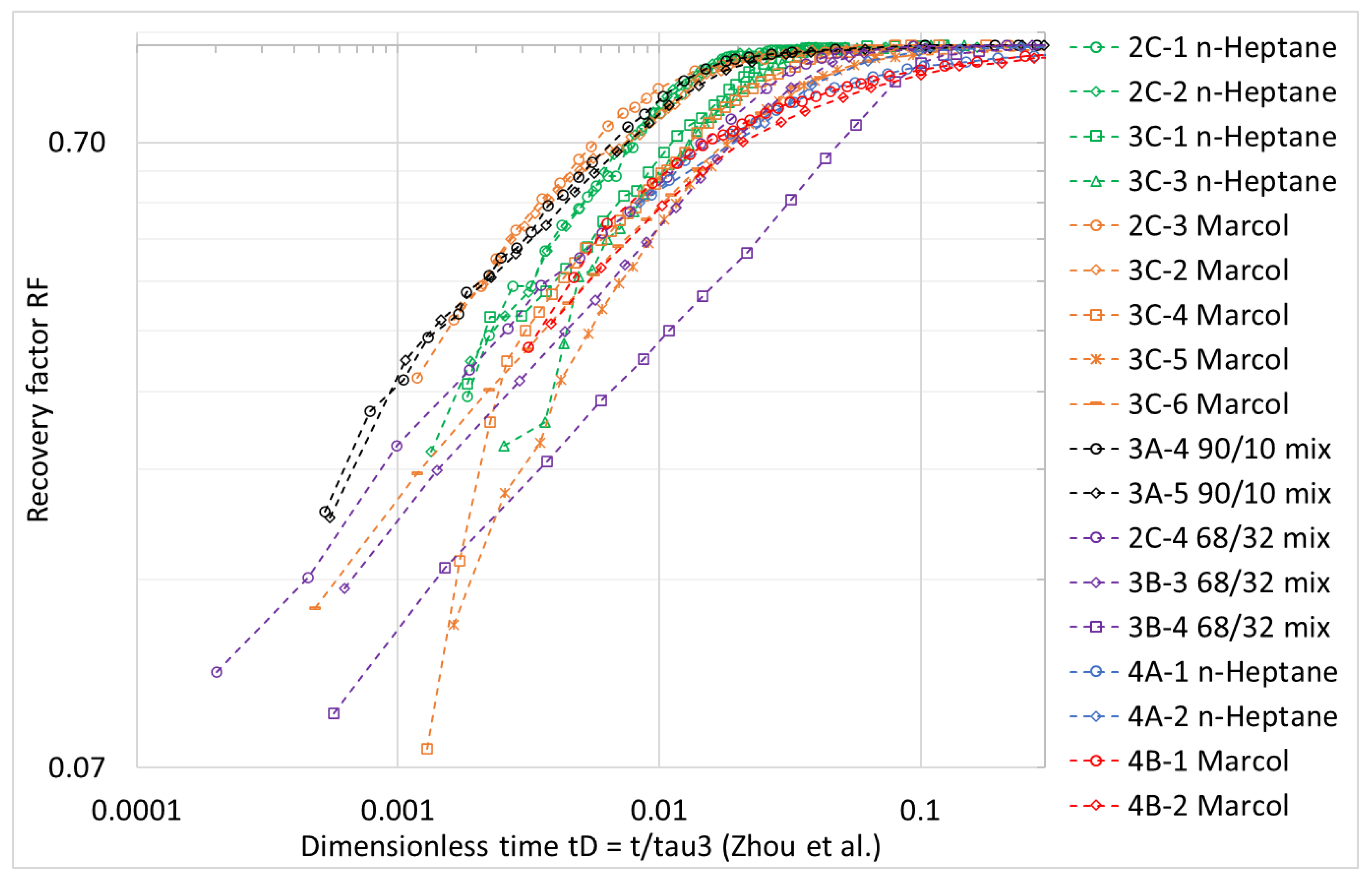
4.2. Spontaneous Imbibition Results

The spontaneous imbibition data are plotted in Figure 3 as average water saturation against logarithmic time. Measurements at times less than a minute were considered inaccurate and are not included. The fastest imbibition experiments are the Bentheimer cores (4A and B), which have a magnitude higher permeability than the Berea cores. The ~80 times higher oil viscosity with Marcol over heptane increases the time scale by a factor between three and ten for the Bentheimer tests. The variation between C7 and M82 tests for Berea is similar, roughly a factor of five. The saturations obtained are mainly consistent, with some exceptions. Bentheimer tests reach s w ~ 0.6 , while Berea tests tended to reach s w ~ 0.47 . The C7 tests reached slightly less water imbibition, s w ~ 0.44 for Berea, but not for Bentheimer.
Next, the data are presented in scaled form. When scaling (with τ 1 , τ 2 or τ 3 ), each experiment was scaled using its individually measured values (of s w i , s o r , k r o * , etc). The same permeability was assumed for a given core. Values not measured for a given test were estimated from the average measurements of the other tests on the same rock type.
RF is plotted against t / τ 1 in log–log format in Figure 4. The modified Mattax and Kyte time scale τ 1 eliminates the role of core dimensions, permeability, saturation range, porosity and IFT (the water viscosity was the same). Many of the tests display linear trends in the log–log format indicating infinite-acting behavior, especially for intermediate recovery values (see the purple, black, green, orange curves). These trends are less clear for Bentheimer and the early time data for several Berea tests; where the time since the onset of imbibition was short. The Bentheimer tests with Marcol (red curves) clearly demonstrate declining slopes in the log–log format after about RF = 0.5 suggesting the end of infinite acting behavior. The heptane data of Bentheimer seem to enter this period at a higher recovery ~0.7. This is in line with getting a higher recovery factor in the infinite acting domain when oil has a higher mobility [48].
Although the curves are scaled, the Bentheimer data have ~2–3 times shorter scaled times than Berea under same experimental conditions (compare the Marcol tests and Heptane tests) indicating some difference in the saturation functions. For a given rock type, and assuming the (normalized) saturation functions are the same, this figure directly shows the influence of varying the oil viscosity while other effects are eliminated. For both rock types we see that changing Heptane to Marcol increases the time by a factor ~5. The 90/10 oil mixture had ~10 times higher viscosity than heptane, which increased the time from heptane by ~3. The 68/32 mixture had ~30 times higher viscosity than heptane, and the time increase was on average similar to Marcol compared to heptane, ~5, but with some variation.
In Figure 5 we use Ma et al. [29]’s time scale τ 2 to present the data. This time scale also attempts to correct for the role of viscosities by assuming the imbibition time increases proportionally with μ w μ o . When changing oil from heptane to Marcol the oil viscosity increases by a factor ~80, which should increase the time by a factor ~9, roughly one order of magnitude. As we have just explained, such great changes in time scale were not observed and the scaling leads to an overcorrection. The low viscosity cases (heptane) using τ 2 now have over half an order of magnitude larger scaled time than the high viscosity cases (Marcol) and the data overall are less collected, now scattered by roughly one order of magnitude, while in Figure 5 the scatter was roughly within ~0.7 log units of scaled time. This demonstrates a more complex influence of viscosities on the time scale than given by the geometric mean.
We previously found that the water relative permeability end point was much lower than the oil relative permeability end point, which is likely to influence the imbibition experiments. The relative permeability end points and viscosities are combined in Zhou et al. [37]’s time scale τ 3 by evaluating the oil and water mobilities at their end points in the diffusion coefficient. The scaled data are shown in Figure 6. The Berea experiments were collected closely within a half order of magnitude, although one outlier (3B-4) was seen. The scatter in the scaled experiments is of the same magnitude as the scatter in experiments under the same conditions: for example, the orange curves were all performed on Berea cores with Marcol. Similarly, the purple curves represent Berea cores with 68/32 mix. In both cases the scaled times spanned a half order of magnitude at a given RF.
We note that no measurements had been made of k r w * for Bentheimer. This parameter was estimated based on the premise that all the curves should overlap when accounting for their characteristic mobility. Assuming the same value as the average of the Berea (flooding) tests (0.012) led to a slightly shorter scaled time than the Berea data but with overlap. Values 0.03 < k r w * < 0.10 put the Bentheimer data within the range of the Berea data (not considering the outlier 3B-4) and the value k r w * = 0.065 was selected.

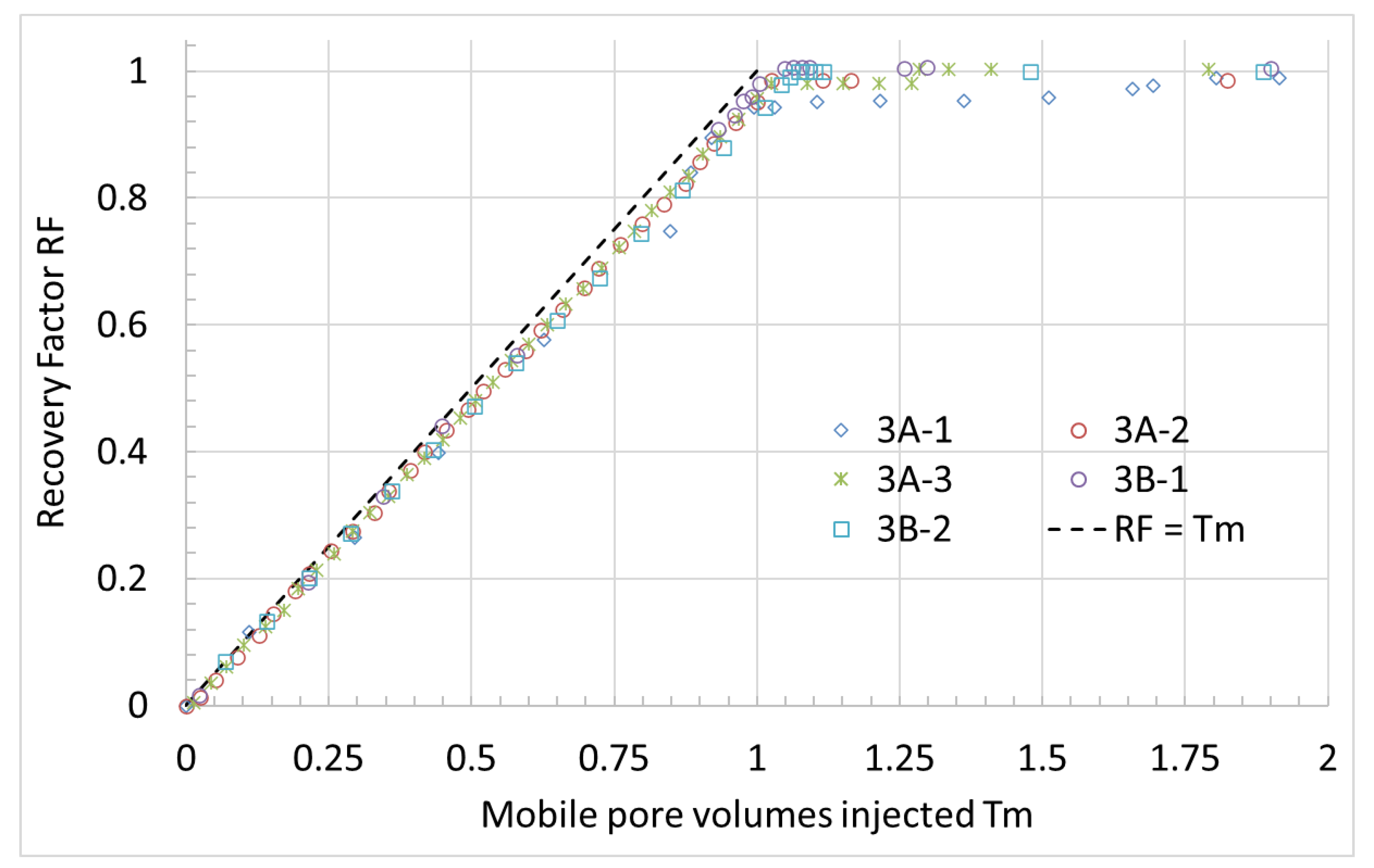
4.3. Forced Imbibition Data

Recovery RF is plotted against mobile pore volumes T m = T / Δ s w in Figure 7. The data for all five tests fall on the predicted straight line R F = T m (<5% under) from (17) until full recovery when one mobile pore volume has been injected, although test 3A-1 had some late production. Overall, the linear recovery until full production indicated piston-like production for all the tests, for all combinations of oil viscosity and injection rate. As calculated in Table 3, all the mobility ratios are below one (in the range 0.0056 to 0.42).
We next consider normalized pressure drop Δ p / Δ p r e f together with the predicted straight line obtained from (22) when the capillary pressure term is ignored. This line starts from M (based on fluid viscosities and k r o * and k r w * obtained at oil and water flow, respectively) and ends at one. The data are shown for heptane (C7) tests in Figure 8 and Marcol (M82) tests in Figure 9.
In all cases the pressure drop increased with time, in line with a favorable mobility ratio. Even when oil had much higher viscosity than brine, the low k r w * gave water lower mobility than oil. The data were mainly below the straight line. This indicates that capillary forces aided the imbibition process since less pressure drop was required than piston-like displacement without capillary forces. The pressure drop increased faster with time, towards the water end point. In Figure 9 left, a similar set of relative permeability end points were measured, and same fluids were used, but different injection rates. The high-rate experiment 3A-2 shows data closer to the straight line and the data are more linear, in line with expected behavior at dominating advective forces. The second low-rate experiment in the right figure is also significantly below the straight line. We expected similar impact of rate for the heptane experiments in Figure 8, but there appeared to be similar or less deviation from the straight line at a low rate. The measured k r w * was ~2.5 times lower in the low-rate experiment 3B-2 than 3B-1, which increases advective forces at the given rate and balances the impact of rate reduction.

4.4. Matching Experimental Data

To model the experiments, some experimental properties were averaged to represent many tests with one model. For flooding, L was given the average length of the flooded cores 3A and 3B; for spontaneous imbibition L c was given the average characteristic length based on all the cores. The same s w i , k r o * , σ , μ w were used in all cases, while s o r , ϕ , K , k r w * were set based on rock type (Berea or Bentheimer). μ o was set according to oil. The parameters in the k r i and J functions were assumed the same for all tests except that k r w * differed between Berea and Bentheimer (as determined from flooding and scaling, respectively). We apply extended Corey relative permeability correlations [51]:
k r w = k r w * S n w , k r o = k r o * ( 1 S ) n o
n w = n w 1 S + n w 2 ( 1 S ) , n o = n o 1 S + n o 2 ( 1 S )
The exponents n w , n o can vary with saturation to better match data. The J -function is a modified Bentsen and Anli [52] type correlation:
J ( S ) = J 1 ln ( S ) + J 2 ln ( 1 S + Δ S Δ S ) ,     d J d S = J 1 S J 2 1 S + Δ S
This is defined such that J ( S = 1 ) = 0 , as expected for SWW media. The slope goes to negative infinity at S = 1 + Δ S and the function can be made steeper near S = 1 with a lower Δ S .
Initial imbibition relative permeability and J functions were taken from Kleppe and Morse [15] who measured on a 290 mD and 22.5% porosity Berea sandstone with 30% initial water saturation. The saturation range was normalized, and the relative permeability end points adapted to our observations. Further tuning was conducted primarily of the Corey exponents and magnitude of the J -function to match the time scale and shape of the heptane and Marcol SI experiments, and the recovery and scaled pressure profiles of the FI Berea tests. An overview of the simulation input parameters is given in Table 4. The matched functions are compared to the literature curves in Figure 10, where the main difference is that the matched Berea water relative permeability and the J -function are lower.
The match of the spontaneous imbibition experiments is shown in Figure 11 for Berea and Bentheimer tests with heptane and Marcol. The time scale of the experiments, their relative difference (due to viscosity), and the recovery at which the infinite acting period ends is well captured. Note, for example, that the high viscosity (Marcol) experiments are modeled to last 3–5 times longer than their corresponding low viscosity (heptane) tests and the Marcol tests end the linear recovery at a lower recovery level than the heptane tests. These levels are lower for Bentheimer than Berea since the water mobility was higher.
Numerical simulation of the forced imbibition tests on Berea are shown in Figure 12 for heptane ( μ o = 0.41 cP) and Marcol ( μ o = 32 cP). The experimental rates (2 and 15 mL/h) and two more were simulated, corresponding to a range of 3 to 100 PV/d. For both cases a very high recovery is obtained before water breakthrough (~99% with heptane and ~95% with Marcol). This is similar to the experimental observations, see Figure 7. Changing the rate had very little impact on the recovery profiles: it followed the linear trend R F = T m followed by a plateau with low oil rate after water breakthrough. A third case was simulated with 150 cP to see the behavior when the mobility ratio became unfavorable, M 2.18 in the example. Breakthrough occurs at R F ~ 0.9 .
At high injection rates (as capillary forces are suppressed) the normalized pressure drop profiles converge to straight line profiles against injected mobile pore volumes. The lines start at the mobility ratio M and end at one for piston-like displacement (seen for heptane) and either higher value (Markol) or lower (150 cP oil) if the imbibing profile has less and more mobility than flowing water, respectively. The profiles were shifted lower if the rate was reduced, which indicates that capillary forces spontaneously act as a separate driving force to imbibe water.
When the water reaches the outlet, the saturation front carrying the capillary driving force, vanishes and a corresponding viscous pressure drop must be added to maintain the rate. This is seen as a sharp jump in pressure drop for both heptane and Marcol simulation cases. However, the pressure drop was not significantly reduced for the 150 cP case, but showed a peak higher than that obtained with low capillary forces (high rate). Furthermore, for Markol, the peak was higher with capillary forces (low rate). This indicates that capillary forces can also add resistance during the displacement. We note that the increased oil viscosity reduces the relative importance of capillary forces.
To better understand the role of capillary pressure during injection, we consider water saturation distributions for the cases with low (0.41 cP) and high (150 cP) oil viscosity in Figure 13. The profiles are compared at same number mobile pore volumes injected, but at high and low injection rates, corresponding to low and high importance of capillary forces, respectively. For high and low viscosity cases, capillary forces smear the profiles at low rate. This causes the inlet saturation to not build up to its maximum mobile saturation until after some time. With low oil viscosity, water imbibition reduces the mobility in the system and eventually the pressure drop must be increased to sustain the rate beyond what the spontaneous imbibition provides. The pressure drop increases linearly with T m after that to sustain the rate (Figure 12). The jump in pressure drop at T m = 0.98 is associated with water reaching the outlet and saturations increasing to almost eliminate the capillary pressure driving force. For the high viscosity case, the Buckley–Leverett profile has a lower mobility than the oil and the pressure drop reduces with time. Although the saturation profile visibly changes by capillary forces, the pressure drop appears close to unaffected, even with the low rate of 0.6 mL/h. High viscosity and non-uniform saturation profile reduces the capillary driving force, see (23). The main impact of the capillary forces is seen at water arrival at the outlet, with a jump in pressure drop. Water accumulates to reach zero capillary pressure, which halts breakthrough. This reduces the mobility of the oil and increases the pressure drop. Considering the net effect of smearing and accumulation, slightly earlier breakthrough appears to result when capillary forces are present. This can also be seen for the Markol simulation on close inspection.

4.5. Viscosity Impact on Spontaneous Imbibition Behavior

Based on the determined saturation functions for Berea, we are interested in the effect of viscosity in a SWW system. To compare oil and water viscosity fairly, we let them have reference values of 1 cP (black curve) and vary them individually (red curves for oil and blue curves for water). The resulting plot of RF against the square root of time is shown in Figure 14. Increasing water viscosity increases the imbibition time much more than increasing oil viscosity, resulting from the low water mobility, which limits the imbibition rate. For example, increasing water viscosity by 100 increases the time by ~36, while the same change in oil viscosity increases the time only by ~5.5. It is also demonstrated that the level of recovery reached in infinite-acting mode (linear with the square root of time) depends on the mobilities. As the mobility of oil increases compared to that of water (by increasing water viscosity) this level is increased towards full recovery. Similarly, by reducing the mobility of oil relative to water (by increased oil viscosity) the RF reached in this regime falls (from 0.93 in the reference case to 0.70 with 100 cP oil viscosity). This supports the prediction from the analytical model (27) stating that as the oil mobility becomes large relative to that of water, a more piston-like displacement results where the recovery profile follows the square root of time until all the mobile oil is recovered.

5. Summary and Conclusions

Counter-current spontaneous imbibition experiments were conducted both on strongly water-wet Berea and Bentheimer sandstone and forced imbibition was conducted on Berea. High and low oil viscosity (varying by a factor of 80) were used, and the injection rate varied from 2–15 mL/h. Consistent interpretation of the experiments revealed that water had much lower relative permeability than oil, both in terms of low end points and high Corey exponents and that significant positive capillary forces were present. These features were required to explain observations in the spontaneous imbibition recovery profiles, and the forced imbibition recovery and pressure drop profiles. Analytical models were derived to explain the role of capillary forces and favorable mobility ratio during the two imbibition modes.
  • During flooding, linear recovery vs. volume injected was observed until all mobile oil was displaced for high and low combinations of rate and viscosity indicating piston-like displacement. This was explained by a favorable mobility ratio even at high oil viscosities. Capillary pressure effects gave less recovery at breakthrough as the effect of capillary diffusion towards the outlet was greater than the capillary water blockage effect.
  • Pressure drop should increase linearly with time from the oil end point mobility to the water end point mobility if piston-like displacement occurs. If it is lower than this trend, capillary forces assist the imbibition. The pressure drop increases in a jump at water breakthrough as the capillary pressure contribution, mainly at the front, vanishes.
  • Non-piston-like displacement will also give a pressure drop changing linearly with time, but the end point depends on the mobility of the imbibing saturation profile and when it reaches the outlet. Capillary blockage at that time can cause an added resistance with a pressure peak higher than without capillary forces.
  • The change in spontaneous imbibition time scale ~3–5 was much less than the change in oil viscosity (a factor ~80), and indicated that oil mobility was much higher than that of water.
  • Including relative permeability end points during the scaling of spontaneous imbibition data provided much better results in terms of collecting the imbibition curves than only using the viscosities. That was due to the water relative permeability being very low compared to oil. The scaling was successfully used to estimate the water relative permeability end point for Bentheimer.
  • The time scale of spontaneous imbibition is more sensitive to water viscosity than oil viscosity in a SWW system since water has the limiting mobility. When oil mobility becomes increased compared to the water mobility, a higher recovery will be obtained following a square root of time profile, with the entire profile as a limiting case of infinite oil mobility.
The implications of these findings are that mobile oil is effectively displaced both by forced and spontaneous imbibition in SWW media, where piston-like displacement is a reasonable approximation unless the oil viscosity is much higher than that of water. In both modes, very little tail production is expected after the end of the linear production regime against time and the square root of time, respectively. Determining intermediate relative permeability from water flooding will be challenging since the end saturations dominate the saturation profile within the core. However, the end point water relative permeability and residual oil saturation will be obtained fast, since just one mobile pore volume is needed, and accurately, since capillary end effects do not cause water accumulation at a steady state in a SWW system.
Although several conditions were tested to understand imbibition in SWW media, we emphasize the value of exploring a wider range of viscosities, rates and boundary conditions, to see, e.g., when water flooding becomes non-piston-like and verify the difference in impacts of oil and water viscosity on time scale. Water can also imbibe spontaneously in a co-current fashion and display a complex behavior. Some findings of this study may also change if the wettability is not SWW, but mixed- or oil-wet. In the latter case, capillary forces may resist flooding and increase the pressure drop, rather than reducing it.

Author Contributions

Conceptualization, P.Ø.A.; Methodology, P.Ø.A. and D.S.S.; Validation, L.S. and D.S.S.; Formal analysis, P.Ø.A.; Investigation, L.S. and D.S.S.; data curation, L.S. and D.S.S.; writing—original draft preparation, P.Ø.A., L.S. and D.S.S.; writing—review and editing, P.Ø.A. All authors have read and agreed to the published version of the manuscript.

Funding

This research received no external funding.

Institutional Review Board Statement

Not applicable.

Informed Consent Statement

Not applicable.

Data Availability Statement

The data can be shared upon request.

Acknowledgments

Andersen acknowledges the Research Council of Norway and the industry partners of NCS2030—RCN project number 331644—for their support.

Conflicts of Interest

The authors declare no conflict of interest.

Nomenclature

Roman
D  Diameter: m
f w  Water fractional flow function
J  Scaled capillary pressure
J 1 , J 2 , Δ S J -function parameters
k r i  Phase relative permeability
K  Absolute permeability, m2
L  Core length, m
L c  Characteristic length, m
M  End point mobility ratio
n i  Phase Corey exponent
n i 1 , n i 2  Phase Corey exponent end values
p i  Phase pressure, Pa
P c  Capillary pressure, Pa
R F  Recovery factor (of mobile oil)
s i  Phase saturation
S i  Normalized phase saturation
S e q  Normalized water saturation, at which capillary pressure is zero
S ¯  Normalized water saturation averaged over the core
T  Scaled time
T m  Mobile pore volumes injected
u i  Darcy phase velocity, m/s
Greek
ϕ  Porosity
μ i  Phase viscosity, Pa s
σ o w  Interfacial tension, N/m
λ i  Phase mobility, 1/(Pa s)
Δ p i  Phase pressure drop, Pa
Δ p r e f  Pressure drop when water flows at residual oil saturation, Pa
Δ s w  Mobile saturation range
τ  Time scale, s
Subscripts
c  Capillary
c h  Characteristic
e q  Zero capillary pressure condition
f  Front
i  Phase index
o  Oil
r  Reference (no end effects)
T  Total
w  Water
Superscripts
*  End point or characteristic value

Appendix A. Forced Imbibition with Buckley–Leverett Profile

Consider that the saturation profile is unaffected by the capillary diffusion term in (2). The saturation profile is then described by the solution of Buckley and Leverett [53]:
x ( s w ) = u T t ϕ f ( s w ) = T m L Δ s w f ( s w ) , ( s f < s w < 1 s o r ) ,
x f = u T t ϕ f ( s w f ) = T m L Δ s w f ( s w f ) , ( s w r < s w < s f ) ,
The notation refers to saturation differentiation. s f is the front saturation, determined by solving:
f w ( s f ) = f w ( s f ) f w ( s w r ) s f s w r , ( s f [ s w r , 1 s o r ] )
The profile can be separated into the continuous BL solution behind the front, 0 < x < x f , with nonzero saturation gradient, and the profile ahead of the front x f < x < L where the saturation is constant at initial water saturation. Scale position relative to xf the front:
X = x x f ( t ) = f w ( s w ) f w ( s f ) ,     d X = d x x f ( t )
The total Darcy velocity in the two regions, expressed with water pressure, is given by:
u T = K λ T ( s w ) 1 x f X p w K λ o ( s w ) 1 x f X P c ( s w ) , ( 0 < X < 1 )
u T = K λ o ( s w r ) 1 x f X p w , ( 1 < X < L x f )
The outlet oil pressure is zero, p o R = 0 . Water is immobile ahead of the front and its pressure is determined by the initial capillary pressure before reaching the outlet, p w = p o P c ( s w r ) ,   ( X > 1 ) . The inlet pressures are equal p L = p w L = p o L (as the highest mobile saturation is at the inlet) and equals the measured pressure drop Δ p . The pressure gradients in each region are:
X p w = λ o λ T X P c x f u T K λ T , ( 0 < X < 1 )
X p w = x f u T K λ o ( s w r ) , ( 1 < X < L x f )
The pressure gradient is constant in the oil region. The pressure drops in the two intervals are calculated:
p w f p w L = σ o w ϕ / K X = 0 1 ( 1 f w ) X J d X x f u T K X = 0 1 1 λ T d X ,
p w R p w f = u T K λ o ( s w r ) ( L x f ) ,
p w f is the water pressure at x f . For known viscosities and functions k r w , k r o , J ; f w and λ T are known and the integrals are constant independent of front position and time, denoted:
Δ J * = X = 0 1 ( 1 f w ) X J d X > 0 ,     1 λ T * = X = 0 1 1 λ T d X > 0
We make use of the boundary conditions, eliminate p w f and combining the equations to obtain pressure drop Δ p = p w L as function of front position:
Δ p = u T K [ x f λ T * + ( L x f ) λ o ( s w r ) ] σ o w ϕ / K [   J ( s w r ) Δ J * ]
The front position x f is related to u T by (A2), which inserted into (A12) gives:
Δ p = u T L K ( 1 λ o ( s w r ) + T m ( 1 λ T * 1 λ o ( s w r ) ) Δ s w f ( s w f ) ) σ o w ϕ / K [   J ( s w r ) Δ J * ]
Scaling the equation with the reference pressure drop results in:
Δ p Δ p r e f = ( M + T m ( λ w * / λ T * M ) Δ s w f w ( s w f ) ) λ w * σ o w v T L K / ϕ (   J ( s w r ) Δ J * ) ,

References

  1. Blunt, M.J. Multiphase Flow in Permeable Media: A Pore-Scale Perspective; Cambridge University Press: Cambridge, UK, 2017. [Google Scholar]
  2. Ahmed, T. Reservoir Engineering Handbook; Gulf Professional Publishing: Cambridge, MA, USA, 2018. [Google Scholar]
  3. Morrow, N.R. Wettability and its effect on oil recovery. J. Pet. Technol. 1990, 42, 1476–1484. [Google Scholar] [CrossRef]
  4. Johnson, E.F.; Bossler, D.P.; Naumann, V.O. Calculation of relative permeability from displacement experiments. Trans. AIME 1959, 216, 370–372. [Google Scholar] [CrossRef]
  5. Jones, S.C.; Roszelle, W.O. Graphical techniques for determining relative permeability from displacement experiments. J. Pet. Technol. 1978, 30, 807–817. [Google Scholar] [CrossRef]
  6. Civan, F.; Donaldson, E.C. Relative permeability from unsteady-state displacements: An analytical interpretation. In SPE Production Operations Symposium; OnePetro: Moscow, Russia, 1987. [Google Scholar]
  7. Leverett, M. Capillary behavior in porous solids. Trans. AIME 1941, 142, 152–169. [Google Scholar] [CrossRef]
  8. Andersen, P.Ø.; Walrond, K.; Nainggolan, C.K.; Pulido, E.Y.; Askarinezhad, R. Simulation interpretation of capillary pressure and relative permeability from laboratory waterflooding experiments in preferentially oil-wet porous media. SPE Reserv. Eval. Eng. 2020, 23, 230–246. [Google Scholar] [CrossRef]
  9. Rapoport, L.A.; Leas, W.J. Properties of linear waterfloods. J. Pet. Technol. 1953, 5, 139–148. [Google Scholar] [CrossRef]
  10. Gupta, R.; Maloney, D.R. Intercept method—A novel technique to correct steady-state relative permeability data for capillary end effects. SPE Reserv. Eval. Eng. 2016, 19, 316–330. [Google Scholar] [CrossRef]
  11. Andersen, P.Ø. Analytical modeling and correction of steady state relative permeability experiments with capillary end effects–An improved intercept method, scaling and general capillary numbers. Oil Gas Sci. Technol. Rev. D’ifp Energ. Nouv. 2021, 76, 61. [Google Scholar] [CrossRef]
  12. Anderson, W.G. Wettability literature survey-part 4: Effects of wettability on capillary pressure. J. Pet. Technol. 1987, 39, 1283–1300. [Google Scholar] [CrossRef]
  13. Craig, F. The Reservoir Engineering Aspects of Waterflooding; Monograph Series; Society of Petroleum Engineers of AIME: Wilkes-Barre, PA, USA, 1971. [Google Scholar]
  14. Anderson, W.G. Wettability literature survey-part 6: The effects of wettability on waterflooding. J. Pet. Technol. 1987, 39, 1605–1622. [Google Scholar] [CrossRef]
  15. Kleppe, J.; Morse, R.A. Oil production from fractured reservoirs by water displacement. In Proceedings of the Fall meeting of the Society of Petroleum Engineers of AIME, Houston, TX, USA, 6–9 October 1974. [Google Scholar]
  16. Anderson, W.G. Wettability literature survey part 5: The effects of wettability on relative permeability. J. Pet. Technol. 1987, 39, 1453–1468. [Google Scholar] [CrossRef]
  17. Bourbiaux, B.J.; Kalaydjian, F.J. Experimental study of cocurrent and countercurrent flows in natural porous media. SPE Reserv. Eng. 1990, 5, 361–368. [Google Scholar] [CrossRef]
  18. Yortsos, Y.C.; Fokas, A.S. An analytical solution for linear waterflood including the effects of capillary pressure. SPE J. 1983, 23, 115–124. [Google Scholar] [CrossRef]
  19. Odeh, A.S.; Dotson, B.J. A method for reducing the rate effect on oil and water relative permeabilities calculated from dynamic displacement data. J. Pet. Technol. 1985, 37, 2051–2058. [Google Scholar] [CrossRef]
  20. Morrow, N.R.; Mason, G. Recovery of oil by spontaneous imbibition. Curr. Opin. Colloid Interface Sci. 2001, 6, 321–337. [Google Scholar] [CrossRef]
  21. Amott, E. Observations relating to the wettability of porous rock. Trans. AIME 1959, 216, 156–162. [Google Scholar] [CrossRef]
  22. Handy, L.L. Determination of effective capillary pressures for porous media from imbibition data. Trans. AIME 1960, 219, 75–80. [Google Scholar] [CrossRef]
  23. Mason, G.; Morrow, N.R. Developments in spontaneous imbibition and possibilities for future work. J. Pet. Sci. Eng. 2013, 110, 268–293. [Google Scholar] [CrossRef]
  24. Andersen, P.Ø.; Brattekås, B.; Nødland, O.; Lohne, A.; Føyen, T.L.; Fernø, M.A. Darcy-Scale simulation of Boundary-Condition effects during Capillary-Dominated flow in high-permeability systems. SPE Reserv. Eval. Eng. 2019, 22, 673–691. [Google Scholar] [CrossRef]
  25. Haugen, Å.; Fernø, M.A.; Mason, G.; Morrow, N.R. The effect of viscosity on relative permeabilities derived from spontaneous imbibition tests. Transp. Porous Media 2015, 106, 383–404. [Google Scholar] [CrossRef]
  26. Andersen, P.Ø. Early-and Late-Time Analytical Solutions for Cocurrent Spontaneous Imbibition and Generalized Scaling. SPE J. 2021, 26, 220–240. [Google Scholar] [CrossRef]
  27. Andersen, P.Ø.; Ahmed, S. Simulation study of wettability alteration enhanced oil recovery during co-current spontaneous imbibition. J. Pet. Sci. Eng. 2021, 196, 107954. [Google Scholar] [CrossRef]
  28. Mattax, C.C.; Kyte, J.R. Imbibition oil recovery from fractured, water-drive reservoir. SPE J. 1962, 2, 177–184. [Google Scholar] [CrossRef]
  29. Ma, S.; Morrow, N.R.; Zhang, X. Generalized scaling of spontaneous imbibition data for strongly water-wet systems. J. Pet. Sci. Eng. 1997, 18, 165–178. [Google Scholar]
  30. Fischer, H.; Morrow, N.R. Scaling of oil recovery by spontaneous imbibition for wide variation in aqueous phase viscosity with glycerol as the viscosifying agent. J. Pet. Sci. Eng. 2006, 52, 35–53. [Google Scholar] [CrossRef]
  31. Mason, G.; Fischer, H.; Morrow, N.R.; Ruth, D.W. Correlation for the effect of fluid viscosities on counter-current spontaneous imbibition. J. Pet. Sci. Eng. 2010, 72, 195–205. [Google Scholar] [CrossRef]
  32. Tantciura, S.; Qiao, Y.; Andersen, P.Ø. Simulation of Counter-Current Spontaneous Imbibition Based on Momentum Equations with Viscous Coupling, Brinkman Terms and Compressible Fluids. Transp. Porous Media 2022, 141, 49–85. [Google Scholar] [CrossRef]
  33. Zhou, X.; Morrow, N.R.; Ma, S. Interrelationship of wettability, initial water saturation, aging time, and oil recovery by spontaneous imbibition and waterflooding. SPE J. 2000, 5, 199–207. [Google Scholar] [CrossRef]
  34. McWhorter, D.B.; Sunada, D.K. Exact integral solutions for two-phase flow. Water Resour. Res. 1990, 26, 399–413. [Google Scholar] [CrossRef]
  35. Standnes, D.C. Scaling spontaneous imbibition of water data accounting for fluid viscosities. J. Pet. Sci. Eng. 2010, 73, 214–219. [Google Scholar] [CrossRef]
  36. Standnes, D.C.; Andersen, P.Ø. Analysis of the impact of fluid viscosities on the rate of countercurrent spontaneous imbibition. Energy Fuels 2017, 31, 6928–6940. [Google Scholar] [CrossRef]
  37. Zhou, D.; Jia, L.; Kamath, J.; Kovscek, A.R. Scaling of counter-current imbibition processes in low-permeability porous media. J. Pet. Sci. Eng. 2002, 33, 61–74. [Google Scholar] [CrossRef]
  38. Schmid, K.S.; Geiger, S. Universal scaling of spontaneous imbibition for arbitrary petrophysical properties: Water-wet and mixed-wet states and Handy’s conjecture. J. Pet. Sci. Eng. 2013, 101, 44–61. [Google Scholar] [CrossRef]
  39. Andersen, P.Ø.; Nesvik, E.K.; Standnes, D.C. Analytical solutions for forced and spontaneous imbibition accounting for viscous coupling. J. Pet. Sci. Eng. 2020, 186, 106717. [Google Scholar] [CrossRef]
  40. Reis, J.C.; Cil, M. A model for oil expulsion by counter-current water imbibition in rocks: One-dimensional geometry. J. Pet. Sci. Eng. 1993, 10, 97–107. [Google Scholar] [CrossRef]
  41. Tavassoli, Z.; Zimmerman, R.W.; Blunt, M.J. Analytic analysis for oil recovery during counter-current imbibition in strongly water-wet systems. Transp. Porous Media 2005, 58, 173–189. [Google Scholar] [CrossRef]
  42. Churcher, P.L.; French, P.R.; Shaw, J.C.; Schramm, L.L. Rock properties of Berea sandstone, Baker dolomite, and Indiana limestone. In Proceedings of the SPE International Symposium on Oilfield Chemistry, Anaheim, CA, USA, 20–22 February 1991. [Google Scholar]
  43. Peksa, A.E.; Wolf, K.H.A.; Zitha, P.L. Bentheimer sandstone revisited for experimental purposes. Mar. Pet. Geol. 2015, 67, 701–719. [Google Scholar] [CrossRef]
  44. Hamouda, A.A.; Valderhaug, O.M.; Munaev, R.; Stangeland, H. Possible mechanisms for oil recovery from chalk and sandstone rocks by low salinity water (LSW). In Proceedings of the SPE Improved Oil Recovery Symposium, Tulsa, OK, USA, 12–16 April 2014. [Google Scholar]
  45. Abhishek, R.; Hamouda, A.A.; Murzin, I. Adsorption of silica nanoparticles and its synergistic effect on fluid/rock interactions during low salinity flooding in sandstones. Colloids Surf. A Physicochem. Eng. Asp. 2018, 555, 397–406. [Google Scholar] [CrossRef]
  46. Andersen, P.Ø.; Qiao, Y.; Standnes, D.C.; Evje, S. Cocurrent spontaneous imbibition in porous media with the dynamics of viscous coupling and capillary backpressure. SPE J. 2019, 24, 158–177. [Google Scholar] [CrossRef]
  47. Lenormand, R.; Lorentzen, K.; Maas, J.G.; Ruth, D. Comparison of four numerical simulators for SCAL experiments. Petrophysics 2017, 58, 48–56. [Google Scholar]
  48. Andersen, P.Ø. Early- and late-time prediction of counter-current spontaneous imbibition and estimation of the capillary diffusion coefficient. In Proceedings of the SPE EuropEC, Madrid, Spain, 5–9 June 2022. [Google Scholar]
  49. Fischer, H.; Wo, S.; Morrow, N.R. Modeling the Effect of Viscosity Ratio on Spontaneous Imbibition. SPE Reserv. Eval. Eng. 2008, 11, 577–589. [Google Scholar] [CrossRef]
  50. Lohne, A. User’s Manual for BugSim–an MEOR Simulator (V1.2); NORCE: Stavanger, Norway, 2013. [Google Scholar]
  51. Brooks, R.H.; Corey, A.T. Properties of porous media affecting fluid flow. J. Irrig. Drain. Div. 1966, 92, 61–90. [Google Scholar] [CrossRef]
  52. Bentsen, R.G.; Anli, J. A new displacement capillary pressure model. J. Can. Pet. Technol. 1976, 15. [Google Scholar] [CrossRef]
  53. Buckley, S.E.; Leverett, M. Mechanism of fluid displacement in sands. Trans. AIME 1942, 146, 107–116. [Google Scholar] [CrossRef]
Figure 1. Simplified illustrations of the applied spontaneous (left) and forced (right) imbibition setups. Blank arrows indicate water flow, while dark arrows indicate oil flow.
Energies 15 03531 g001
Figure 2. Two of the cores used in the experiments seen from the end face and side. Core 3B is of Berea type, while core 4A is Bentheimer type.
Energies 15 03531 g002
Figure 3. Spontaneous imbibition results of water saturation s w plotted against time t .
Energies 15 03531 g003
Figure 4. Spontaneous imbibition results of recovery factor RF plotted against scaled time t / τ 1 (time scaled using the modified time scale of Mattax and Kyte [28] including Ma et al.’s characteristic length).
Energies 15 03531 g004
Figure 5. Spontaneous imbibition results of RF plotted against scaled time t / τ 2 , where τ 2 is Ma et al. [29]’s time scale. Compared to the previous figure, oil viscosity is assumed scaled via μ w μ o .
Energies 15 03531 g005
Figure 6. Spontaneous imbibition results of RF plotted against scaled time t / τ 3 where τ 3 is the time scale by Zhou et al. [37] and accounts for fluid viscosities and relative permeability end points.
Energies 15 03531 g006
Figure 7. Recovery factor RF plotted against mobile pore volumes injected for all the forced imbibition tests. All the tests indicate piston-like displacement of oil by water.
Energies 15 03531 g007
Figure 8. Normalized pressure drop Δ p / Δ p r e f plotted against mobile pore volumes injected for the forced imbibition tests with Heptane, C7 (0.41 cP) at low rate (blue points) and high rate (red points). The data are compared with the predicted model (dashed lines) of piston-like displacement with no end effects.
Energies 15 03531 g008
Figure 9. Normalized pressure drop Δ p / Δ p r e f plotted against mobile pore volumes injected for the forced imbibition tests with Marcol (32 cP) at low rate (blue points) and high rate (red points). The data are compared with the predicted model (dashed lines) of piston-like displacement with no end effects.
Energies 15 03531 g009
Figure 10. Saturation functions plotted against normalized saturations for data based on [15], and adaptations to match the experimental results in this work. Lower J-function and lower water relative permeability for Berea were required to match our data. The J values can be converted into capillary pressure with the factor σ ϕ / K = 44.7 kPa for Berea.
Energies 15 03531 g010
Figure 11. Comparison of experimental spontaneous imbibition results for Berea (left) and Bentheimer (right) against simulated results considering only the experiments with heptane and Markol. The time is scaled with τ 1 to account for variations in core dimension, permeability, porosity and end saturations.
Energies 15 03531 g011
Figure 12. Simulated recovery factor (left) and normalized pressure drop (right) plotted against mobile pore volumes injected for Berea input parameters using oil viscosity of heptane 0.41 cP (top), Markol 32 cP (middle) and a synthetic high value 150 cP (bottom). The * mark denotes a characteristic value.
Energies 15 03531 g012
Figure 13. Saturation distributions after different number mobile pore volumes injected T m as indicated for oil viscosity of 0.41 cP (left) and 150 cP (right) using Berea saturation functions. High rate (HR) corresponds to 60 mL/h, while low rate (LR) corresponds to 2 mL/h for low viscosity and 0.6 mL/h for high viscosity.
Energies 15 03531 g013
Figure 14. Simulated recovery factor plotted against square root of time based on Berea saturation functions and different phase viscosities, indicated for water (w) and oil (o) in cP. The green points indicate where the curves stop to be linear.
Energies 15 03531 g014
Table 1. Overview of fluid properties: (1) Viscosity and density are reported at 20 °C. All values used in calculations were corrected for actual temperature during experiment; (2) IFT is between oil and 1 M NaCl. The oil mixtures ‘90/10’ and ‘68/32’ refer to oil mixtures of heptane/Marcol.
n-Heptane
(C7)
C7-M82
Mixture
(90/10)
C7-M82
Mixture
(68/32)
Marcol 82
(M82)
1 M
NaCl
0.1 M
NaCl
1 Viscosity [cP]0.4084.0413.8231.771.0980.965
Viscosity ratio μ o μ w 0.393.8913.3130.59
1 Density [g/mL]0.6840.8000.8330.8501.03861.0024
2 Interfacial tension [mN/m]35.4035.0538.2039.51--
Table 2. Measured core properties. 1 Subject to 10 bar net confining pressure. 2 Calculated from measurements of bulk and grain volumes at atmospheric pressure.
Core IDSource L D L c V b V m V p =
V b V m
V p       1 ϕ     2 K g       1
[mm][mm][mm][mL][mL][mL][mL][%][mD]
2CBerea59.3137.8012.1866.5653.1013.4613.1519.85152
3A 64.9437.8212.3672.9558.6414.3113.9319.19124
3B 64.0737.8212.3471.9857.7814.2013.7819.25126
3C 65.6137.8212.3873.7159.2114.5014.1319.26128
4ABentheimer67.4237.6412.3875.0256.2318.7918.6324.271989
4B 65.9437.6212.3373.3055.1018.2018.0725.581948
Table 3. Overview of performed tests, imbibition type (forced FI or spontaneous SI), nonwetting phase used, initial water saturation, relative permeability end points (not measured in all tests) and the rates used in FI tests. Cores two and three are Berea and core four is Bentheimer type. For SI tests the s o r was estimated by the highest oil saturation. The ‘relative variation’ is given as two standard deviations divided by the average.
Core IDImbibition
Type
NW
Phase
s w i [ frac ]
k o ( s w i ) [ mD ]
k r o ( s w i ) [ frac ]
s o r [ frac ]
k w ( s o r ) [ mD ]
k r w ( s o r ) [ frac ]
M
[-]
Rate
[mL/h]
Berea
2C-1SIC70.100--0.561-- -
2C-2SIC70.098--0.559-- -
2C-3SIM820.100--0.509-- -
2C-4SI68-320.1021220.8050.505-- -
3A-1FIM820.1041020.8230.5711.410.01140.422
3A-2FIM820.10187.10.7020.5451.190.00960.4215
3A-3FIM820.10390.50.7300.5190.7880.00640.272
3A-4SI90-100.100--0.514-- -
3A-5SI90-100.104100.40.8110.507-- -
3B-1FIC70.10681.70.6480.5852.900.02300.013815
3B-2FIC70.10383.20.6600.5641.190.00940.00562
3B-3SI68-320.101--0.521-- -
3B-4SI68-320.103-0.6770.521-- -
3C-1SIC70.099--0.594-- -
3C-2SIM820.1041110.8670.515-- -
3C-3SIC70.1031000.7810.557-- -
3C-4SIM820.1041030.8050.612-- -
3C-5SIM820.102--0.528-- -
3C-6SIM820.09994.60.7390.520-- -
Average 0.10297.770.7540.5411.500.0120
Rel variation 0.040.250.190.121.091.07
Bentheimer
4A-1SIC70.105--0.403-- -
4A-2SIC70.10413090.6580.396-- -
4B-1SIM820.102--0.398-- -
4B-2SIM820.10514990.7700.446-- -
Average 0.10414040.7140.411
Rel variation 0.030.190.220.12
Table 4. Input parameters used for simulating the experimental data. The values are averaged as follows: L from 3A and 3B (only the flooded cores), L c from all cores (all were used for SI), σ o w for all four oils (the values were similar).
Constant ParametersRock Specific ParametersSaturation Function Parameters
BereaBentheimer TuningK and M
L 64.8 mm s o r 0.540.41 n w 1 66
L c 12.3 mm ϕ 0.1940.249 n w 2 32.5
D 37.75 mm K 133 mD1970 mD n o 1 1.52
σ o w 37.0 mN/m k r w * 0.0120.065 n o 2 1.50.5
μ w 1.10 cP τ 1 5.43 × 10⁻⁴ h2.18 × 10−4 h J 1 0.140.3
μ o [ C 7 ] 0.41 cP J 2 0.0140.03
μ o [ M 82 ] 32 cP Δ S -3 × 10⁻⁴
s w i 0.10 k r o * -0.75
k r o * 0.75 k r w * -0.07
M [ C 7 ] 0.0047
M [ M 82 ] 0.45
Publisher’s Note: MDPI stays neutral with regard to jurisdictional claims in published maps and institutional affiliations.

