Customer-Centric, Two-Product Split Delivery Vehicle Routing Problem under Consideration of Weighted Customer Waiting Time in Power Industry

Abstract

This paper introduces a new model of the customer-centric, two-product split delivery vehicle routing problem (CTSDVRP) in the context of a mixed-flow manufacturing system that occurs in the power industry. Different from the general VRP model, the unique characteristics of our model are: (1) two types of products are delivered, and the demand for them is interdependent and based on a bill of materials (BOM); (2) the paper considers a new aspect in customer satisfaction, i.e., the consideration of the production efficiency on the customer side. In our model, customer satisfaction is not measured by the actual customer waiting time, but by the weighted customer waiting time, which is based on the targeted service rate of the end products. We define the targeted service rate as the ratio of the quantity of the end product produced by the corresponding delivery quantities of the two products to the demand of the end product. We propose a hybrid ant colony-genetic optimization algorithm to solve this model with actual data from a case study of the State Grid Corporation of China. Finally, a case study is explored to assess the effectiveness of the CTSDVRP model and highlight some insights. The results show that the CTSDVRP model can improve customer satisfaction and increase the average targeted service rate of the end products effectively.

1. Introduction

This study is motivated by the following two aspects. On the one hand, the impact of the COVID-19 pandemic combined with rising trade protectionism has led to a severe challenge to the global supply chain currently, that is supply chain shortages. There is a deficit of parts used to make products, such as the computer chips that go into everything from electronics to automobiles. According to a CNN Business report in October 2021, Apple had manufacturing disruption due to supply shortages of chips. A severe shortage of computer chips used to make vital components of vehicles has delayed automotive production and forced some plants to shut down. Moreover, consulting firm AlixPartners forecasts that the lack of chips, coupled with a raft of other raw material shortages, will cut vehicle production by 7.7 million units [1]. In addition, according to the Institute for Supply Management (ISM) Report on Business, there was a shortage of 26 kinds of commodities in the U.S. in October 2021. Due to the shortage of raw materials, the delivery time of suppliers to manufacturers was extended. In October 2021, the average lead time for production materials was 96 days, and the average lead time for Maintenance, Repair and Operating (MRO) supplies was 49 days, which were the longest since ISM began collecting these data in 1987 [2]. Therefore, in the case of supply chain shortages, manufacturers are facing the difficulty of stopping production lines due to a lack of key components, resulting in longer delivery times and customer dissatisfaction.

On the other hand, this study is also motivated by two types of product distribution problems faced by State Grid in China. State Grid is the largest utility enterprise, ranking second among the Fortune Global 500 in 2021. A branch company of State Grid operates a two-echelon inventory system that consists of a central warehouse and multiple secondary warehouses. At the beginning of each month, the manager of each secondary warehouse reports the demands for different types of electric energy metering devices to the central warehouse. State Grid, as a centralized and group-level purchaser, regularly acquires electric energy metering devices from suppliers to meet these demands. Electric energy metering devices must pass a quality test in the central warehouse before being used. Only tested and qualified devices can be delivered to the secondary warehouses. Many kinds of electric energy metering devices are stored in the central warehouse, including single-phase electric energy meters, three-phase electric energy meters, current transformers, voltage transformers, terminals, and concentrators. The central warehouse has a mixed verification flow-shop that can text different types of devices. In most routine businesses, the combination of two types of electric energy metering devices is required by the electrical power station because of their functional complementarity. For example, to build a three-phase three-wire circuit, two current transformers and one three-phase electric energy meter are needed. To build a three-phase four-wire circuit, three current transformers and one three-phase electric energy meter are needed. Thus, the delivery of multiple types of electric energy metering devices is common in the electric power industry. Besides, a similar example can also be observed in the timber-trade industry. A timber-trade company picks up wooden products (e.g., spruce, maple, and pine) from sawmills and serves many wood-processing businesses (delivery points). The wood-processing businesses (delivery points) periodically require different kinds of wooden products to produce a mixture of products (e.g., plywood, panels, and OSB boards) [3]. Therefore, the distribution of multiple types of products is common, and such combinations have to be considered in the delivery process.

The manufacturer’s lead-time may be uncertain, and the capacity for quality tests is limited. When demand surges short-term, a supply shortage of metering devices often occurs and customers’ demands cannot be met at once. Therefore, deliveries need to be split, which causes extra work for both the central and the secondary warehouse. This problem is common in many low-volume and high-mix industries, such as complete equipment manufacturing or system maintenance like State Grid. Industrial manufacturers often have difficulties obtaining the parts they need for production. Customers have to accept the shortage and multiple deliveries, which reduces their satisfaction.

In today’s competitive environment, customer satisfaction plays an important role in a manufacturer’s success. One important aspect that increases customer satisfaction is quick product delivery. Research on customer-centric vehicle routing problems (VRPs) has attracted great attention from researchers and decision-makers, whose objectives are to minimize customer waiting time [4,5]. When measuring customer satisfaction, actual customer waiting time is regarded as one of the most vital criteria. Generally, the shorter the actual waiting time, the higher the satisfaction. However, is this expectation reasonable in the two-product split delivery vehicle routing problem?

Customers who require two interdependent products usually find split deliveries undesirable unless the value of each delivery reaches a certain level of satisfaction. Generally, manufacturers create the BOM that contains the parts needed for the end product [6]. For example, a manufacturer needs two types of parts to produce the end product and orders them from the supplier. The manufacturer cares about not only the actual waiting time, but also the quantities of the end product produced by the corresponding delivery quantities of the two parts. Therefore, in the two-product split delivery vehicle routing problem, we believe that it is unreasonable to measure customer satisfaction only by the actual waiting time. Furthermore, overemphasizing the total customer waiting time ignores the fact that manufacturers often choose to start production as soon as the parts are received in the first delivery while waiting for incoming parts to waste less time and resources. Moreover, waiting for all parts before starting production would cause the logistics service system to become inefficient.

The following example, in which we mainly consider the quantities of completed tasks, illustrates a customer’s satisfaction. One customer needs to install 100 three-phase three-wire circuits, which require 200 current transformers and 100 electric energy meters according to its BOM. We assume that the customer has no inventory of the two types of devices that are stock-in-transit before the first delivery. We consider two possible split delivery situations. Scenario 1: The customer receives 150 current transformers and 50 electric energy meters in the first delivery. This means that 50 installations can be completed, and we can say that the value of the first delivery is 50. Scenario 2: The customer receives 180 current transformers and 20 electric energy meters in the first delivery, so only 20 tasks can be completed, and the value is 20. In both scenarios, the installation of the three-phase three-wire circuits is interrupted by the lack of electric energy meters before the next delivery. Although the total quantity of delivered items in Scenario 1 is equal to that in Scenario 2 (200 for each), the value of the first delivery in Scenario 1 is greater than that in Scenario 2. In these two situations, customer satisfaction is different. The customer’s actual waiting time is equal in both situations, yet the customer satisfaction in scenario 1 is higher than that in Scenario 2. Therefore, in two-product split delivery VRPs (SDVRPs), a modified objective of customer satisfaction needs to be considered.

The primary research in the SDVRP literature has been on a single product. Motivated by the applications in the electric industry, this paper studies the customer-centric, two-product split delivery vehicle routing problem (CTSDVRP) in a mixed-flow manufacturing situation while considering the weighted customer waiting time. This paper makes the following three main contributions: First, it identifies a new SDVRP variant that considers two types of products and describes customer satisfaction, not by the actual waiting time, but by the weighted customer waiting time. The weighted customer waiting time is calculated by the targeted service rate of end products, which is defined as the ratio of the quantity of the end product produced by the corresponding delivery quantities of the two products to the demand of the end product. The greater the targeted service rate and the smaller the weighted customer waiting time, the greater the customer satisfaction. Second, it proposes a hybrid ant colony-genetic optimization algorithm to solve the model. Finally, it derives its numerical results from a practical application and analyzes the impact of the weight of customer satisfaction on total distribution costs, total weighted customer waiting time, and average targeted service rate, which provides insights for decision-makers.

The remainder of the paper is organized as follows: Section 2 reviews the related literature. Section 3 presents the problem description and mathematical formulation. The proposed algorithm to solve the problem is described in Section 4. Section 5 presents the computational results and a few comparisons. In Section 6, we conclude this study and provide managerial insights.

2. Literature Review

2.1. Split Delivery Vehicle Routing Problem

The split delivery vehicle routing problem (SDVRP) was introduced in the literature by Dror and Trudeau [7]. They showed how split deliveries can result in savings in both total distances traveled and the number of vehicles utilized. For the next decades, a steady trickle of papers on SDVRPs was published. Archetti et al. [8] presented a general overview of all the studied variants of the SDVRP. Several variants of the traditional SDVRP have been explored including SDVRPs with time windows [9,10,11,12,13,14,15], pickups and deliveries [16,17,18,19,20,21], heterogeneous fleets [22,23,24,25,26], and minimum fraction served [27,28,29]. These studies significantly advanced these areas in the field of SDVRPs.

The studies on SDVRP have primarily focused on a single product, and three of their objectives are to efficiently minimize the total number of vehicles, distance traveled, or transportation costs. However, the distribution of multiple types of products is common. Different from previous work, the focus of our study is on the two-product split delivery vehicle routing problem in mixed-flow manufacturing with interdependent demand for two products based on the bill of materials (BOM), and these two products in varying combinations are assembled into an end product at customer locations.

2.2. Vehicle Routing Problem Considering Customer Satisfaction

Increasingly fierce competition has made customer satisfaction a pivotal factor for the success of a firm. Many studies consider customer satisfaction in multiple areas. In customer service, for example, actual customer waiting time is often regarded as a key indicator that alters customer satisfaction. The shorter the actual customer waiting time, the higher customer satisfaction. Many VRPs aim to minimize total travel distance or total distribution costs, yet some VRPs are customer-centric and intend to minimize actual waiting time [4,30]. Moshref-Javadi et al. [5] presented a customer-centric, multi-commodity split delivery vehicle routing problem. In this study, the authors’ objective was to minimize the actual total customer waiting time to increase customer satisfaction. In addition, Huang et al. [31] thought managers should pay more attention to human factors when considering customer satisfaction. They studied the express vehicle scheduling problem and analyzed the perception of customer waiting time from the perspective of cognitive psychology. They built a satisfaction function that reflects the perception of customer waiting time by incorporating fuzzy theory into prospect theory. This and similar studies attempt to maximize customers’ average perceived satisfaction with waiting time and to minimize travel length.

Improving customer satisfaction usually means increasing total distribution costs. For managers, this is an unavoidable tradeoff. Surprisingly few studies have considered this issue. Wu et al. [32] introduced a mathematical model of the open vehicle routing problem (OVRP) based on customer satisfaction with the objective to minimize travel costs and customer waiting time. Fan [33] studied a VRP that involves pickup and delivery and considers customer satisfaction. His objective was to minimize the weighted sum of the total length of vehicle paths and total customer waiting time. Zhang et al. [34] presented a multi-objective vehicle problem with flexible time windows. They also considered the customer satisfaction related to the route, which is represented as a convex function dependent on the vehicle arrival time. They aimed to minimize overall routing costs and maximize overall customer satisfaction. Yu et al. [35] established a multi-objective delivery model for fresh food with a low distribution cost and high customer satisfaction.

The primary studies on SDVRP considering customer satisfaction also have been on a single product. The goal is to minimize the total customer waiting time when measuring customer satisfaction. Few studies have focused on the multiple types of products, but they did not consider the interdependency between multiple types of products.

We summarize the core literature in Table 1. In summary, our paper studies a customer-centric, two-product split delivery vehicle routing problem (CTSDVRP). Different from previous studies, our model considers the weighted customer waiting time when evaluating the customer satisfaction. Due to split deliveries and the interdependency of two products, we calculated the weighted customer waiting time based on the targeted service rate of end products. The targeted service rate is defined as the ratio of the quantity of the end product produced by the corresponding delivery quantities of the two products to the demand of the end product. The objective of our model is to minimize the weighted sum of the total distribution cost and the total losses of the weighted customer waiting time.

Table 1. Objectives of the reviewed literature.

Author	Multi-Products	Distribution Cost Objective		Customer Satisfaction Objective
		Total Travel Cost	Other Costs	Customer Waiting Time	Weighted Customer Waiting Time
Ho et al. [9]		√	√
Salani et al. [10]		√
Luo et al. [11]		√
Fu et al. [13]		√	√
Li et al. [14]		√
Lespay et al. [15]			√
Qiu et al. [17]		√
Wolfinger et al. [20]		√
Zhang et al. [21]	√	√
Gschwind et al. [18]	√	√
Tavakkoli et al. [22]		√	√
Belfiore et al. [23]		√
Wang et al. [26]		√
Hertz et al. [24]		√	√
Han et al. [28]		√
Nucamendi et al. [30]				√
Martínez et al. [4]				√
Moshref et al. [5]	√			√
Huang et al. [31]				√	√
Wu et al. [32]				√
Fan [33]				√
Zhang et al. [34]				√
Yu et al. [35]		√		√
This paper	√	√		√	√

3. Problem Description and the Mathematical Model

3.1. Problem Description

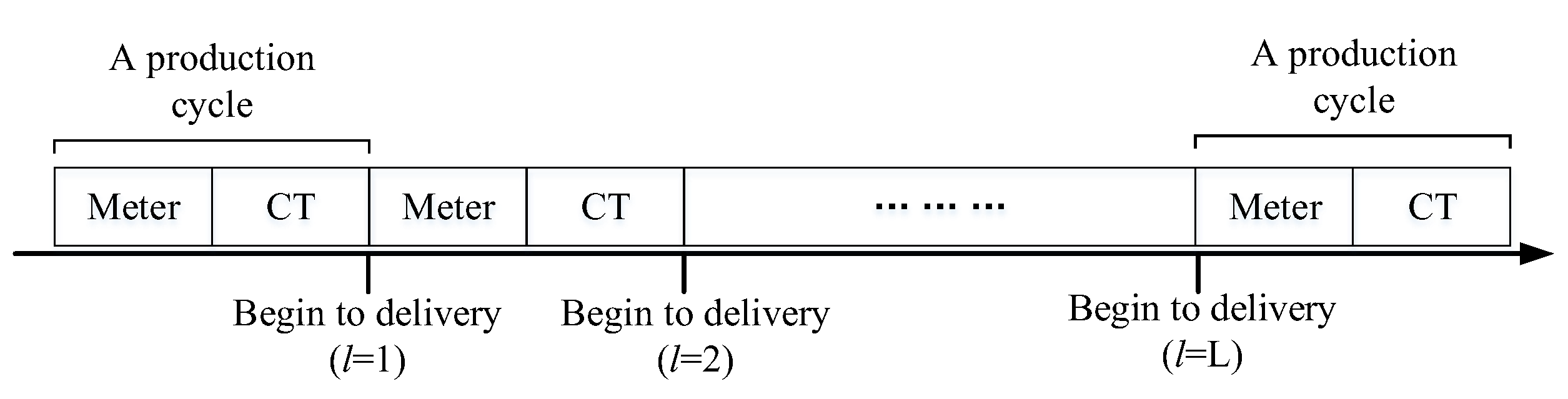
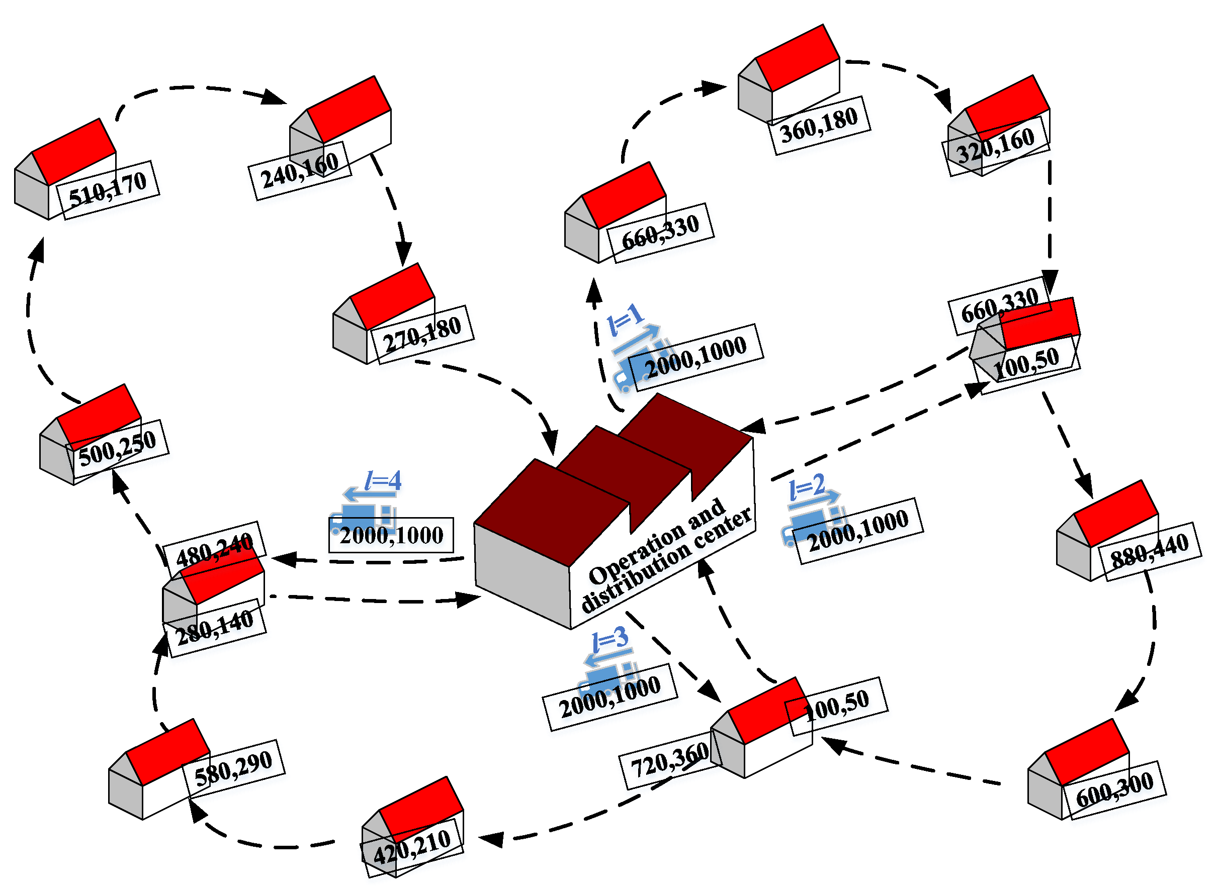
The problem analyzed in our study is derived from a real-life product distribution problem of State Grid, a government-owned power company in China. A branch company of State Grid has a mixed verification flow-shop that can verify different types and quantities of electric energy metering devices. Generally, the combination of two types of electric energy metering devices is required for the customer due to their functional complementarity, and the demand for them is based on the BOM. Assume that two types of electric energy metering devices need to be verified in the mixed verification flow-shop: an electric energy meter (Meter) and a current transformer (CT). As shown in Figure 1, Meters and CTs are verified in succession. We define a production cycle as one completed round of Meter and CT verification. In each production cycle, the manager determines the verification quantities of Meters and CTs. When a production cycle is finished, the delivery of Meters and CTs starts. Furthermore, we have a set of delivery times $R=\left\{1,2,\cdots ,L\right\},l\in R,t\in R$. For each delivery, the company sends one vehicle. In such a case, the delivery vehicle routing problem of the interdependent two-product is required. Figure 2 illustrates the problem in which there is one central warehouse that distributes two types of products to multiple customers, which is the problem that our paper studied.

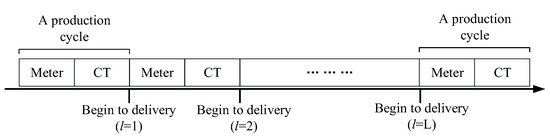
Figure 1. Mixed verification and distribution timing.

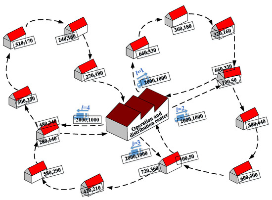
Figure 2. The CTSDVRP schematic description.

The problem is given by a set of customers $M=\left\{1,2,\cdots ,m\right\}$, residing at m different locations where Node 0 denotes the central warehouse. We let $V=M\cup \left\{0\right\}$ denote the set of all nodes. Let i and j be the two nodes in V, where $i,j\in V$ and $i\ne j$. The traveling distance between nodes i and j is denoted $d_{ij}$ and $d_{ij}=d_{ji}$. Assume that the vehicles travel at the same speed, so the traveling time $t_{ij}$ between nodes i and j is symmetric. We assume that customers require two types of products (Meter and CT), referred to here as Product 1 and Product 2, respectively. We denote $N_{1i}$ and $N_{2i}$ ($i=1,2,\cdots ,m$) as customer i’s demand for Product 1 and Product 2, respectively. Customer i ($i=1,2,\cdots ,m$) requires $n_{1i}$ units of Product 1 and $n_{2i}$ units of Product 2 to process one unit of electric end product. Customer i’s demand may be fulfilled with more than one vehicle. In addition, an unlimited number of homogeneous vehicles with capacity a can be used to operate the distribution task [21]. All vehicles leave and return to the central warehouse.

The following notations are defined to formulate the problem; see Table 2.

Table 2. List of notations used in this paper.

Parameters
$N_{1i}$, $N_{2i}$	Customer i’s demand for Product 1 and Product 2
a	The capacity of vehicles
f	The fixed cost of vehicles
$\eta$	Per-unit distance variable cost of vehicles
C	The unit loss cost of customer waiting time
$T_0^l$	The moment at which the vehicle leaves the central warehouse for the lth delivery
$t_{ij}^l$	Travel time from customer i to customer j for the lth delivery
$T_i^0$	The earliest moment at which the customer i can receive service
$s_i^l$	The service time at customer i for the lth delivery
M	Large positive constant
$\alpha$	The weight of the customer satisfaction, $\alpha \in [0,1]$.
Decision Variables
$x_{ij}^l$	Binary variable; 1, if the vehicle travels from customer i to j for the lth delivery; 0, otherwise
$T_i^l$	The moment at which the vehicle arrives at customer i for the lth delivery
$q_{1i}^l$	The quantity of Product 1 delivered to customer i for the lth delivery
$q_{2i}^l$	The quantity of Product 2 delivered to customer i for the lth delivery

3.2. Basic Mathematical Model

In this section, we present two basic mathematical models of the problem: Basic Model 1 and Basic Model 2. The objective of both models is to determine customer satisfaction and distribution costs.

For Basic Model 1, the customer satisfaction is described by actual customer waiting time. The objective functions can be written as follows:

$$\underset{x_{ij}^l,q_{1i}^l,q_{2i}^l}{min}{Y}_1=\alpha C{\displaystyle \sum _{l=1}^L}\sum _{i=1}^m(T_i^l-T_i^{l-1})+(1-\alpha )(fL+{\displaystyle \sum _{l=1}^L}\sum _{i=0}^m\sum _{j=0}^m\eta d_{ij}{x}_{ij}^l)$$

(1)

subject to:

$${\displaystyle \sum _{j=1}^m}{x}_{0j}^l=1\begin{array}{cc};& l=1,2,···,L\end{array}$$

(2)

$${\displaystyle \sum _{i=0}^m}{x}_{ik}^l-{\displaystyle \sum _{j=0}^m}{x}_{kj}^l=0\begin{array}{cc};& k=0,1,2,\cdots ,m\begin{array}{cc};& l=1,2,···,L\end{array}\end{array}$$

(3)

$${\displaystyle \sum _{i=1}^m}\sum _{l=1}^L{x}_{ij}^l\ge 1\begin{array}{cc};& j=0,1,\cdots ,m\end{array}$$

(4)

$${\displaystyle \sum _{l=1}^L}{q}_{1i}^l=N_{1i}\begin{array}{cc};& i=1,2,\cdots ,m\end{array}$$

(5)

$${\displaystyle \sum _{l=1}^L}{q}_{2i}^l=N_{2i}\begin{array}{cc};& i\end{array}=1,2,\cdots ,m$$

(6)

$$N_{1i}{\displaystyle \sum _{j=0}^m}{x}_{ij}^l\ge q_{1i}^l\begin{array}{cc};& i=1,2,\cdots ,m\begin{array}{cc};& l=1,2,···,L\end{array}\end{array}$$

(7)

$$N_{2i}{\displaystyle \sum _{j=0}^m}{x}_{ij}^l\ge q_{2i}^l\begin{array}{cc};& i=1,2,\cdots ,m\begin{array}{cc};& l=1,2,···,L\end{array}\end{array}$$

(8)

$$\sum _{i\in S}\sum _{j\in S}{x}_{ij}^l\le \left|S\right|-1\begin{array}{cc};& S\subseteq M,l=1,2,···,L\end{array}$$

(9)

$${\displaystyle \sum _{i=1}^m}(q_{1i}^l+q_{2i}^l)\le a\begin{array}{cc};& l=1,2,\cdots ,L\end{array}$$

(10)

$$T_i^l+s_i^l+t_{ij}^l-(1-x_{ij}^l)M\le \begin{array}{cc}{T}_j^l;& i\end{array}=0,1,\cdots ,m;j=1,2,\cdots ,m;l=1,2,\cdots ,L$$

(11)

$$x_{ij}^l\in \left\{0,1\right\}\begin{array}{cc};& i=0,1,\cdots ,m\begin{array}{cc};& j=0,1,\cdots ,m\begin{array}{cc};& l=1,2,···,L\end{array}\end{array}\end{array}$$

(12)

$$0\le q_{1i}^l\le N_{1i}\begin{array}{cc};\begin{array}{cc}i=1,2,\cdots ,m;& l=1,2,···,L\end{array}& \end{array}$$

(13)

$$0\le q_{2i}^l\le N_{2i}\begin{array}{cc};\begin{array}{cc}i=1,2,\cdots ,m;& l=1,2,···,L\end{array}& \end{array}$$

(14)

In the objective function (1), the first item denotes total losses related to actual customer waiting time. The second item denotes the total distribution cost, where the total fixed distribution cost is $fL$. Constraints (2) and (3) state that each vehicle leaves the center warehouse, arrives at the customers’ locations, leaves again, and finally, returns to the center warehouse. Constraint (4) guarantees that each customer is served at least once. Constraints (5) and (6) guarantee that each customer’s demand will be fulfilled. Constraints (7) and (8) guarantee that the quantity delivered to each customer in the lth delivery cannot exceed its demand. Constraint (9) guarantees that there will be no subtours. Constraint (10) guarantees that the vehicle capacity will not be exceeded. Constraint (11) guarantees that the moment at which the vehicle leaves customer i plus travel time between customer i and j is equal to the moment at which the vehicle arrives at customer j. Constraint (12) guarantees the decision variables $x_{ij}^l$ are binary. Constraints (13) and (14) guarantee that the decision variables $q_{1i}^l$ and $q_{2i}^l$ are positive.

For Basic Model 2, we consider the weighted customer waiting time to assess customer satisfaction. The weighted customer waiting time is calculated based on the actual waiting time and corresponding service rate. The actual customer waiting time is ${\displaystyle \sum _{t=1}^l}(T_i^l-T_i^{l-1})$ for the lth delivery. The service rate is measured by the total delivery quantities for Product 1 and Product 2, that is $\frac{{\displaystyle \sum _{t=1}^{l-1}}(q_{1i}^{l-1}+q_{2i}^{l-1})}{N_{1i}^{}+N_{2i}^{}}$. We define the weighted customer waiting time as

$${\displaystyle \sum _{l=1}^L}\left[1-\frac{{\displaystyle \sum _{t=1}^{l-1}}(q_{1i}^{l-1}+q_{2i}^{l-1})}{N_{1i}^{}+N_{2i}^{}}\right](T_i^l-T_i^{l-1})$$

The objective function of Basic Model 2 can be written as follows:

$$\underset{x_{ij}^l,q_{1i}^l,q_{2i}^l}{min}{Y}_2=\alpha C{\displaystyle \sum _{l=1}^L}{\displaystyle \sum _{i=1}^m}\left[1-\frac{{\displaystyle \sum _{t=1}^{l-1}}(q_{1i}^{l-1}+q_{2i}^{l-1})}{N_{1i}^{}+N_{2i}^{}}\right](T_i^l-T_i^{l-1})+(1-\alpha )(fL+{\displaystyle \sum _{l=1}^L}{\displaystyle \sum _{i=0}^m}{\displaystyle \sum _{j=0}^m}\eta d_{ij}{x}_{ij}^l)$$

(15)

The constraints are the same as those in Basic Model 1.

3.3. The CTSDVRP Model

Although customer satisfaction is described by the weighted customer waiting time in Basic Model 2, this weighted customer waiting time ignores the functional dependencies of Product 1 and Product 2. However, in Basic Model 2, the total delivery quantities for Product 1 and Product 2 may also affect the quantity of the end product produced by the two products. Therefore, as a benchmark, the existence of Basic Model 2 is necessary. In this section, we modify the weighted customer waiting time and present the CTSDVRP model for the problem where the weighted customer waiting time considers the interdependency of Product 1 and Product 2. We measure the weighted customer waiting time not by the total delivery quantities of the two products, but by the quantity of the end product produced by the two products. What is more, the customer’s inventory quantities of Product 1 and Product 2 will affect the quantity of the end product produced by the two products. Therefore, the weighted customer waiting time will also be affected by the customer’s inventory quantities. In addition, there is a contradiction between customer satisfaction and distribution cost, i.e., achieving high customer satisfaction will significantly increase distribution costs [35]. Managers should fully exploit the customer’s time value based on their inventory level to provide a buffer for the delivery time to save costs. However, not all companies can know their customers’ inventory levels. Therefore, in this part, we first consider a case in which the customers’ inventories of two products are zero before the first delivery begins in the CTSDVRP model. Then, l-1 we consider another case in which the customers’ inventories of two products are positive before the first delivery begins. The objective of the two cases for the CTSDVRP model is to minimize the weighted sum of total distribution costs and total losses related to the weighted customer waiting time.

As described in Section 3.1, customer i requires $n_{1i}$ units of Product 1 and $n_{2i}$ units of Product 2 to produce one unit of the end product. Without considering customers’ inventories of the two products, the demand quantities of the end product produced by the two products is $\frac{N_{1i}^{}}{n_{1i}}$ or $\frac{N_{2i}^{}}{n_{2i}}$ ($\frac{N_{1i}^{}}{n_{1i}}=\frac{N_{2i}^{}}{n_{2i}}$, $i=1,2,\cdots ,m$) units for the customer i. In the first $\left(l-1\right)$ th deliveries, customer i can receive ${\displaystyle \sum _{t=1}^{l-1}}{q}_{1i}^{l-1}$ units of Product 1 and ${\displaystyle \sum _{t=1}^{l-1}}{q}_{2i}^{l-1}$ units of Product 2, so customer i can produce $min\left\{⌊\frac{{\displaystyle \sum _{t=1}^{l-1}}{q}_{1i}^{l-1}}{n_{1i}}⌋,⌊\frac{{\displaystyle \sum _{t=1}^{l-1}}{q}_{2i}^{l-1}}{n_{2i}}⌋\right\}$ units of the end product. The targeted service rate is the ratio of the quantity of the end product produced by the corresponding delivery quantities of the two products to the demand of the end product, that is,

$$min\left\{⌊\frac{{\displaystyle \sum _{t=1}^{l-1}}{q}_{1i}^{l-1}}{n_{1i}}⌋/\frac{N_{1i}}{n_{1i}},⌊\frac{{\displaystyle \sum _{t=1}^{l-1}}{q}_{2i}^{l-1}}{n_{2i}}⌋/\frac{N_{2i}}{n_{2i}}\right\}.$$

We define the weighted customer waiting time as

$${\displaystyle \sum _{l=1}^L}max\left\{1-⌊\frac{{\displaystyle \sum _{t=1}^{l-1}}{q}_{1i}^{l-1}}{n_{1i}}⌋/\frac{N_{1i}}{n_{1i}},1-⌊\frac{{\displaystyle \sum _{t=1}^{l-1}}{q}_{2i}^{l-1}}{n_{2i}}⌋/\frac{N_{2i}}{n_{2i}}\right\}(T_i^l-T_i^{l-1}).$$

The objective function can be written as follows:

$$\begin{gathered} \begin{array}{c}\underset{x_{ij}^l,q_{1i}^l,q_{2i}^l}{min}Y=\alpha C{\displaystyle \sum _{l=1}^L}{\displaystyle \sum _{i=1}^m}max\left\{1-⌊\frac{{\displaystyle \sum _{t=1}^{l-1}}{q}_{1i}^{l-1}}{n_{1i}}⌋/\frac{N_{1i}}{n_{1i}},1-⌊\frac{{\displaystyle \sum _{t=1}^{l-1}}{q}_{2i}^{l-1}}{n_{2i}}⌋/\frac{N_{2i}}{n_{2i}}\right\}(T_i^l-T_i^{l-1})\end{array} \\ +(1-\alpha \left)\right(fL+{\displaystyle \sum _{l=1}^L}{\displaystyle \sum _{i=0}^m}{\displaystyle \sum _{j=0}^m}\eta d_{ij}{x}_{ij}^l) \end{gathered}$$

(16)

The constraints are the same as those in Basic Model 1.

Next, suppose the customer’s inventories of the two products are positive before the first delivery begins. Let $z_{1i}$ and $z_{2i}$ be the initial inventories of Product 1 and Product 2, respectively. The demand quantities of the end product produced by the two products is $\frac{N_{1i}+z_{1i}}{n_{1i}}$ or $\frac{N_{2i}+z_{2i}}{n_{2i}}$ ($\frac{N_{1i}+z_{1i}}{n_{1i}}=\frac{N_{2i}+z_{2i}}{n_{2i}}$, $i=1,2,\cdots ,m$) units for customer i. In the first $\left(l-1\right)$ th deliveries, customer i can also receive ${\displaystyle \sum _{t=1}^{l-1}}{q}_{1i}^{l-1}$ units of Product 1 and ${\displaystyle \sum _{t=1}^{l-1}}{q}_{2i}^{l-1}$ units of Product 2, so customer i can produce $min\left\{⌊\frac{{\displaystyle \sum _{t=1}^{l-1}}{q}_{1i}^{l-1}+z_{1i}}{n_{1i}}⌋,⌊\frac{{\displaystyle \sum _{t=1}^{l-1}}{q}_{2i}^{l-1}+z_{2i}}{n_{2i}}⌋\right\}$ units of the end product. Therefore, the targeted service rate of the end product is

$$min\left\{⌊\frac{{\displaystyle \sum _{t=1}^{l-1}}{q}_{1i}^{l-1}+z_{1i}}{n_{1i}}⌋/\left(\frac{N_{1i}+z_{2i}}{n_{1i}}\right),⌊\frac{{\displaystyle \sum _{t=1}^{l-1}}{q}_{2i}^{l-1}+z_{2i}}{n_{2i}}⌋/\left(\frac{N_{2i}+z_{2i}}{n_{2i}}\right)\right\}.$$

In this case, the objective function can be written as follows:

$$\begin{array}{c}\underset{x_{ij}^l,q_{1i}^l,q_{2i}^l}{min}Y=\alpha C{\displaystyle \sum _{l=1}^L}{\displaystyle \sum _{i=1}^m}max\left\{1-⌊\frac{{\displaystyle \sum _{t=1}^{l-1}}{q}_{1i}^{l-1}+z_{1i}}{n_{1i}}⌋/\left(\frac{N_{1i}+z_{1i}}{n_{1i}}\right),1-⌊\frac{{\displaystyle \sum _{t=1}^{l-1}}{q}_{2i}^{l-1}+z_{2i}}{n_{2i}}⌋/\left(\frac{N_{2i}+z_{2i}}{n_{2i}}\right)\right\}(T_i^l-T_i^{l-1})\\ +(1-\alpha \left)\right(fL+{\displaystyle \sum _{l=1}^L}{\displaystyle \sum _{i=0}^m}{\displaystyle \sum _{j=0}^m}\eta d_{ij}{x}_{ij}^l)\end{array}$$

(17)

Property 1.

The greater the value of $\frac{z_{1i}}{n_{1i}}$ or $\frac{z_{2i}}{n_{2i}}$, the greater the customer’s targeted service rate of the end product.

Proof of Property 1. 

Consider two cases: in the first case, customer i’s initial inventories of Product 1 and Product 2 are $z_{1i}$ and $z_{2i}$ ($\frac{z_{1i}}{n_{1i}}=\frac{z_{2i}}{n_{2i}}$); in the second case, customer i’s initial inventories are $z_{{}_{1i}}^{{}^{\prime }}$ and $z_{{}_{2i}}^{{}^{\prime }}$ ($\frac{z_{1i}^{{}^{\prime }}}{n_{1i}}=\frac{z_{2i}^{{}^{\prime }}}{n_{2i}}$). We assume $z_{1i}>z_{1i}^{{}^{\prime }}$ and $z_{2i}>z_{2i}^{{}^{\prime }}$, then compare the values of $⌊\frac{{\displaystyle \sum _{t=1}^{l-1}}{q}_{1i}^{l-1}+z_{1i}}{n_{1i}}⌋/\left(\frac{N_{1i}+z_{1i}}{n_{1i}}\right)$ and $⌊\frac{{\displaystyle \sum _{t=1}^{l-1}}{q}_{1i}^{l-1}+z_{1i}^{{}^{\prime }}}{n_{1i}}⌋/\left(\frac{N_{1i}+z_{1i}^{{}^{\prime }}}{n_{1i}}\right)$ as follows: $\begin{array}{cc}& ⌊\frac{{\displaystyle \sum _{t=1}^{l-1}}{q}_{1i}^{l-1}+z_{1i}}{n_{1i}}⌋/\left(\frac{N_{1i}+z_{1i}}{n_{1i}}\right)-⌊\frac{{\displaystyle \sum _{t=1}^{l-1}}{q}_{1i}^{l-1}+z_{1i}^{{}^{\prime }}}{n_{1i}}⌋/\left(\frac{N_{1i}+z_{1i}^{{}^{\prime }}}{n_{1i}}\right)\hfill \\ & =n_{1i}\left[\left(⌊\frac{{\displaystyle \sum _{t=1}^{l-1}}{q}_{1i}^{l-1}}{n_{1i}}⌋+\frac{z_{1i}}{n_{1i}}\right)\left(N_{1i}+z_{1i}^{{}^{\prime }}\right)-\left(⌊\frac{{\displaystyle \sum _{t=1}^{l-1}}{q}_{1i}^{l-1}}{n_{1i}}⌋+\frac{z_{1i}^{{}^{\prime }}}{n_{1i}}\right)\left(N_{1i}+z_{1i}\right)\right]\hfill \\ & \begin{array}{c}\begin{array}{c}\end{array}\begin{array}{c}\end{array}\begin{array}{c}\begin{array}{c}\hfill \end{array}\hfill \end{array}\begin{array}{c}\hfill \end{array}/\left[\left(N_{1i}+z_{1i}\right)\left(N_{1i}+z_{1i}^{{}^{\prime }}\right)\right]\end{array}\hfill \\ & =n_{1i}\left(z_{1i}-z_{1i}^{{}^{\prime }}\right)\left(\frac{N_{1i}}{n_{1i}}-⌊\frac{{\displaystyle \sum _{t=1}^{l-1}}{q}_{1i}^{l-1}}{n_{1i}}⌋\right)/\left[\left(N_{1i}+z_{1i}\right)\left(N_{1i}+z_{1i}^{{}^{\prime }}\right)\right]\ge 0\hfill \end{array}$

□

Hence, the targeted service rate of the end product in the first case is higher than that in the second case.

4. Customized Hybrid Ant Colony-Genetic Algorithm

The model described in Section 3 involves solving an NP-hard problem [36]. The approaches to solving vehicle routing problems usually include ant colony optimization (ACO) and a genetic algorithm (GA). As a swarm intelligence optimization algorithm, ACO has the merits of parallel computation, self-learning, and effective information feedback. However, in the initial searching stage with no or little information available, the convergence speed is slow. As a global optimization method, GA has the advantages of self-organization, self-adaption, and good global search ability, and it has a fast converging rate in the early searching process [37]. However, as the search continues, it does not have an effective feedback mechanism and generates a large number of redundant iterations, resulting in low efficiency [38]. By fusing these two algorithms, we can utilize the merits of ACO with parallelism and effective feedback and the advantages of a GA with high initial speed-up convergence and create a hybrid ant colony-genetic optimization algorithm.

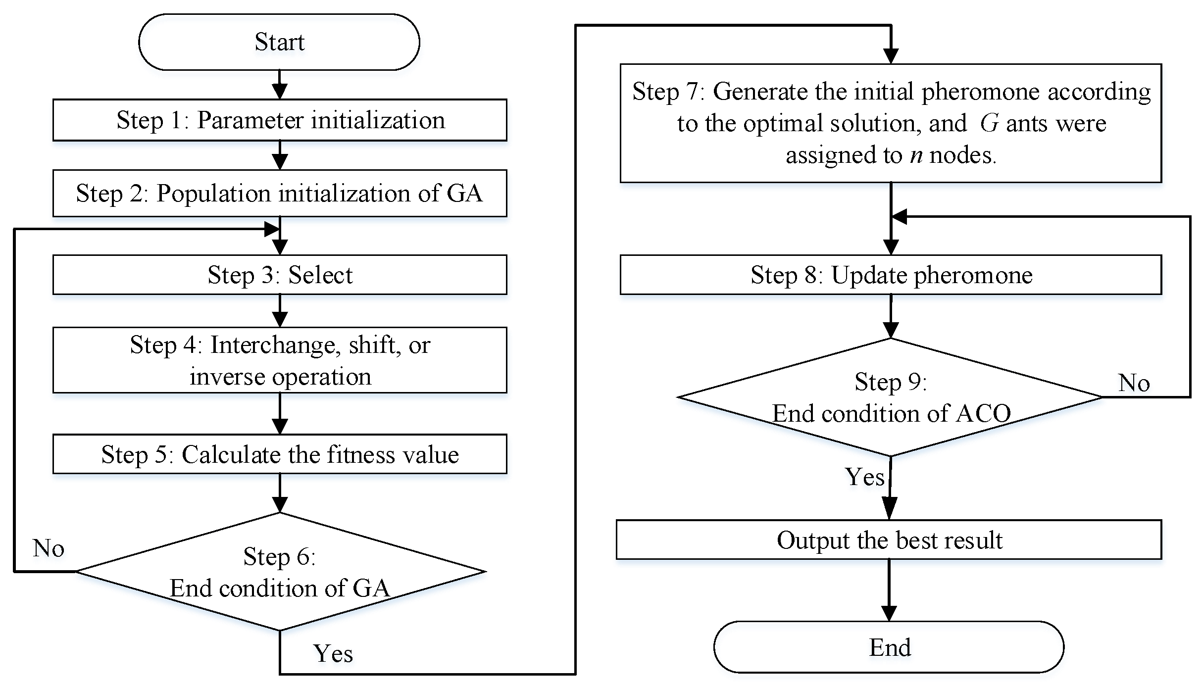
In this paper, the proposed algorithm adopts a GA to generate available solutions based on which they update initial pheromones and then apply ACO to search until the best is reached. The process of a hybrid algorithm of a GA and ACO is shown in Figure 3. The specific steps are as follows:

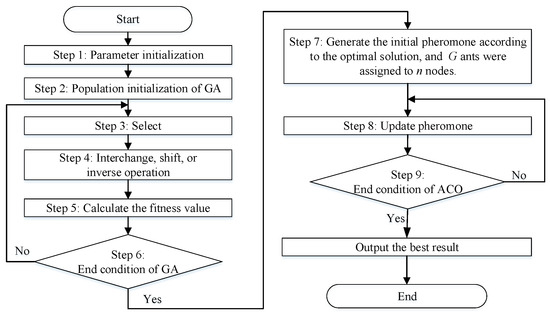
Figure 3. The process of the hybrid ant colony-genetic algorithm.

Step 1: Initialize the control parameters of GA and ACO. For GA, the population size is 100. The Max Iteration is 600. For ACO, the ant number is 100 and the Max Iteration is 400, $\beta =2$, $\gamma =3$, $Q=15$.

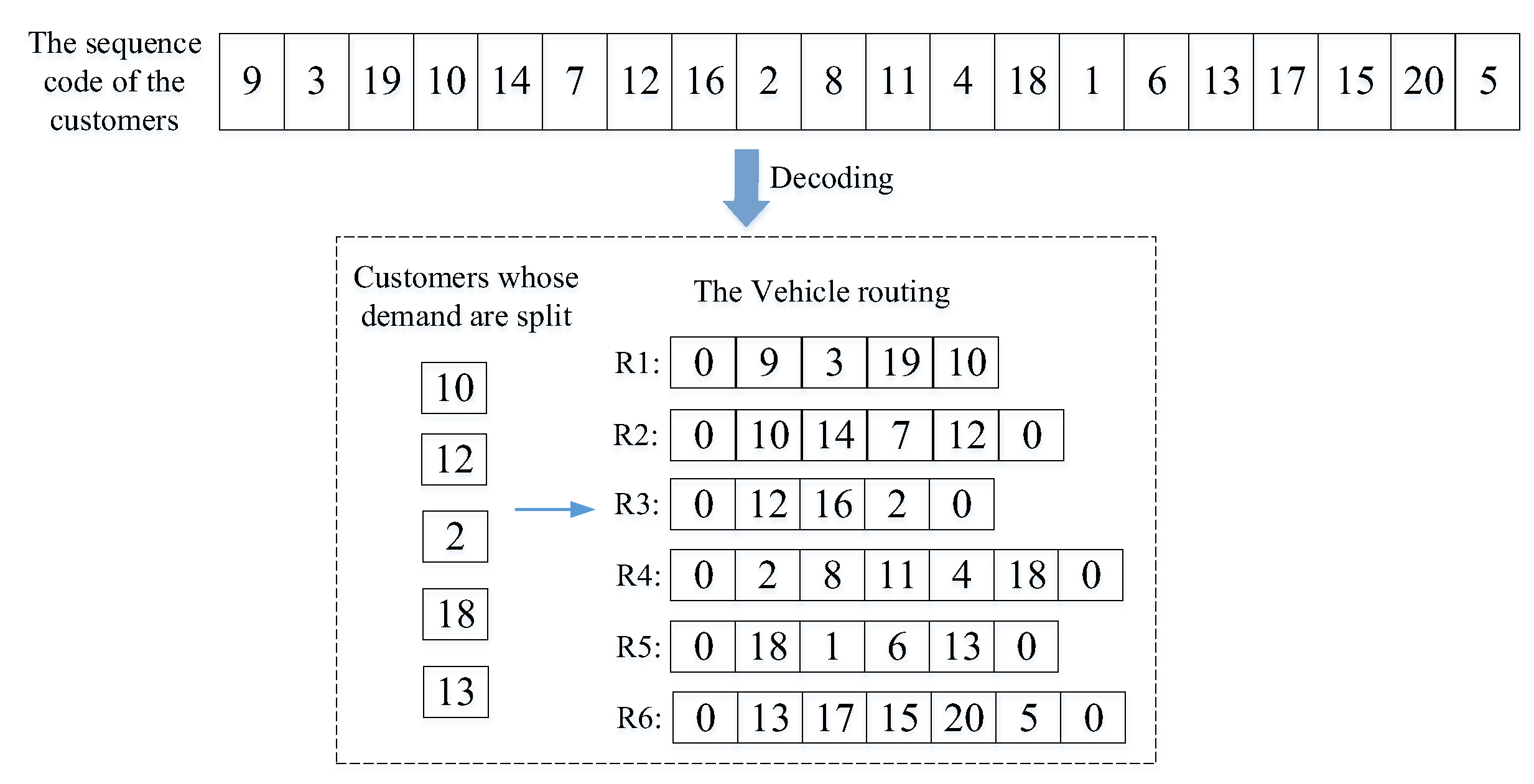
Step 2: Randomly generate the initial population, and set the number of generations. In this paper, natural number coding for customers is used to generate chromosomes. In Figure 4, there are 20 customers (node “1, 2, …, 20”), 1 center depot (Node “0”), and 6 vehicles, and the sequence code of one of the chromosomes is shown. The sequence of the customers is the sequence in which they are served by the vehicle, and the customers are added to the access nodes of the vehicle in turn until the remaining capacity of the vehicle is 0 (assuming that the visited customer point is i at this time). If the current customer i still has unmet demand, the remaining demand of customer i will be met by other vehicles. By analogy, the travel routes of the remaining vehicles can be obtained.

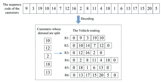
Figure 4. Sequence code and encoding of one chromosome.

Step 3: Select. The resulting population is evenly divided into several groups. Here, every four individuals form a group. The best individuals in each group will be directly retained for the population of the next generation.

Step 4: Realize interchange, shift, or inverse operations. Among the remaining individuals, random methods are used to select genes. After that, the three newly generated individuals in each group will pass on to the next generation. In this paper, interchange, shift, and inverse operations were implemented on the sequence codes of one of the chromosomes.

Step 5: Calculate the fitness of each individual in the population. The fitness function is formulated as the reciprocal of the objective function, i.e., $Fitness=1/Y$, where Y is the objective function value of the basic mathematical models and the CTSDVRP model.

Step 6: Check whether the termination condition of the GA is satisfied. The number of generations is considered to be a termination condition. If it is satisfied, then the process yields the optimal results from the GA and continues to Step 7. Otherwise, it returns to Step 3.

Step 7: Set up the initial pheromone for the ACO according to the results of the GA. We set the searching times and the initial number of ants G and assigned all ants to n nodes. Each ant g visits a customer node following a probabilistic rule prescribed in Equation (18). Customers that are visited by an ant are put into the tabular list. When no further customers can be visited, the ant goes back to the depot and builds the new route.

$$p_{ij}^g=\left\{\begin{array}{cc}\frac{{\tau }_{ij}^{\beta }{\omega }_{ij}^{\gamma }}{{\displaystyle \sum _{s\in N}}{\tau }_{is}^{\beta }{\omega }_{is}^{\gamma }},& j\in N\\ 0& Otherwise\end{array}\right.,$$

(18)

where

$${\omega }_{ij}^{}=1/d_{ij}^{}.$$

(19)

In Equation (18), let $p_{ij}^g$ denote the probability that an ant at node i chooses to next visit node j. Let ${\tau }_{ij}^{}$ represent the value of the pheromone on the arc (i,j). Let ${\omega }_{ij}^{}$ describe the heuristic information. The expected degree of ants moving from node i to node j is ${\omega }_{ij}^{}$. The distance between node i and node j is $d_{ij}$. The control parameters that indicate the importance of the heuristic and pheromone information are $\beta$ and $\gamma$.

Step 8: Pheromone update. In every iteration, the algorithm updates the pheromone information based on Equation (20) given the pheromone evaporation rate $\rho$.

$${\tau }_{ij}^{t^{new}}=(1-\rho ){\tau }_{ij}^{t^{old}}+\Delta {\tau }_{ij}^{t^{old}},\begin{array}{cc}& \end{array}\rho \in (0,1]$$

(20)

In Equation (20), let ${\tau }_{ij}^{t^{new}}$ denote the pheromone information on arc (i,j) in the next iteration. Let ${\tau }_{ij}^{t^{old}}$ denote the current pheromone information on arc (i,j). Let $\Delta {\tau }_{ij}^{t^{old}}$ denote the pheromone that leaves from arc (i,j), which is determined using Equation (21):

$$\Delta {\tau }_{ij}^{t^{old}}={\displaystyle \sum _{g=1}^G}\frac{Q}{L_g}$$

(21)

In Equation (21), Q is a constant parameter for scaling the value of the pheromone contributions. $L_g$ is the total length of the path that ant g has traveled in the current iteration.

Step 9: Check whether the iteration termination condition of the ACO, i.e., the search time, is satisfied. If it is satisfied, the process will yield the best result, and the procedure will end. Otherwise, it returns to Step 8.

5. Case Study

5.1. Background and Data

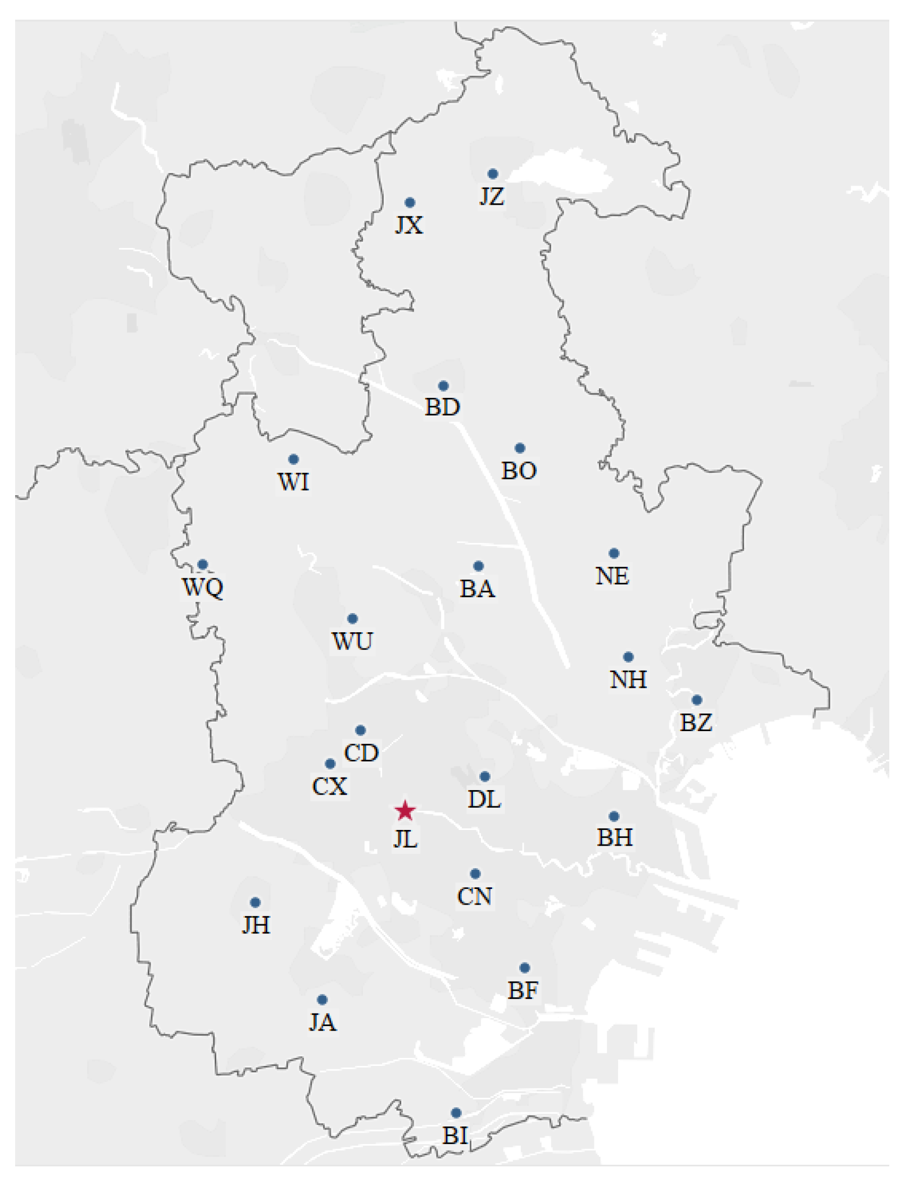
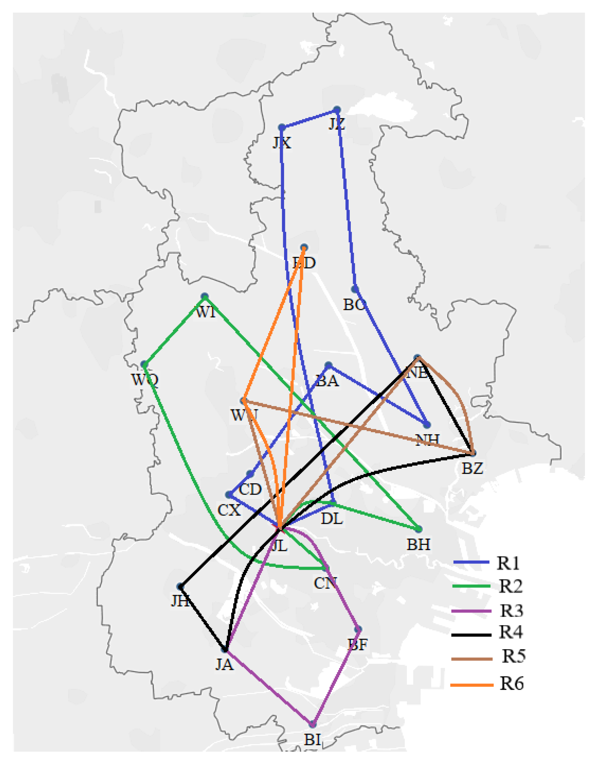
The CTSDVRP model was applied in order to solve a real delivery problem of two types of electric energy metering devices. State Grid tests and supplies electric energy metering devices for multiple secondary warehouses. The location of the company’s center depot (JL) and customers (secondary warehouses) in the city is shown in Figure 5. Let A and B denote the two types of electric energy metering devices. Assume that the testing quantities of A and B in each production cycle are 1000 and 500, respectively. We collected data about the demands of 20 customers for two types of electric energy metering devices. Due to the confidentiality agreement, we preprocessed the original demand data. The processed demand data are shown in Table 3.

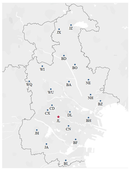
Figure 5. The distribution center and the secondary warehouse locations.

Table 3. The demands and inventories of 20 customers for A and B.

Customer	Demands		Inventories
	A	B	A	B
CD	186	100	30	8
CX	65	45	25	15
CN	175	129	35	11
DL	135	50	30	5
BD	728	368	22	7
BA	102	58	38	12
BO	84	59	56	11
BH	189	146	42	8
BF	261	99	36	0
BZ	658	325	6	7
BI	279	167	0	19
JZ	206	66	34	14
JX	124	58	40	24
JH	522	278	34	0
JA	476	156	10	6
NH	228	71	12	9
NE	399	258	27	26
WQ	257	142	53	13
WU	658	271	155	0
WI	268	154	60	10

We set the related parameters as follows: The delivery vehicle is traveling at a constant speed, and the speed is 60 km/h. The capacity of the delivery vehicle is 1500 devices. The fixed distribution cost is 100 ($f=100$). The unit traveling distance cost is 1 ($\eta =1$). Table 4 and Table 5 show the traveling distance from one customer (or center depot) to the other. State Grid begins to test at 7:00 a.m. The test efficiency is 250 per hour. The total delivery time is 6 ($L=6$). All customers begin to receive service at 9:00 a.m. The unit disutility based on waiting time is 40 ($C=40$). The weight of customer satisfaction is 0.95, i.e., $\alpha =0.95$.

Table 4. Traveling distance matrix among customers.

	JL	CD	CX	CN	DL	BD	BA	BO	BH	BF	BZ
JL	0	15	15	16	14	71	43	63	35	33	52
CD	15	0	8	31	22	59	34	54	45	48	56
CX	15	8	0	31	26	66	41	61	49	47	62
CN	16	31	31	0	17	82	52	72	25	18	47
DL	14	22	26	17	0	66	35	55	23	33	38
BD	71	59	66	82	66	0	31	17	77	98	67
BA	43	34	41	52	35	31	0	21	48	68	43
BO	63	54	61	72	55	17	21	0	63	87	51
BH	35	45	49	25	23	77	48	63	0	30	24
BF	33	48	47	18	33	98	68	87	30	0	54
BZ	52	56	62	47	38	67	43	51	24	54	0
BI	52	66	63	40	57	122	92	112	57	27	80
JZ	107	95	102	117	100	36	65	46	109	133	94
JX	101	88	94	113	96	31	61	45	108	129	96
JH	30	34	26	37	44	92	68	88	62	46	81
JA	35	46	40	33	46	105	77	98	58	34	80
NH	45	46	53	45	31	55	29	39	27	55	14
NE	55	52	59	58	43	40	23	23	44	71	28
WQ	53	38	39	69	59	50	46	56	81	87	86
WU	33	19	24	47	34	42	23	40	55	65	59
WI	62	47	51	76	62	28	36	38	80	93	78

Table 5. Traveling distance matrix among customers (continued from Table 4).

	BI	JZ	JX	JH	JA	NH	NE	WQ	WU	WI
JL	52	107	101	30	35	45	55	53	33	62
CD	66	95	88	34	46	46	52	38	19	47
CX	63	102	94	26	40	53	59	39	24	51
CN	40	117	113	37	33	45	58	69	47	76
DL	57	100	96	44	46	31	43	59	34	62
BD	122	36	31	92	105	55	40	50	42	28
BA	92	65	61	68	77	29	23	46	23	36
BO	112	46	45	88	98	39	23	56	40	38
BH	57	109	108	62	58	27	44	81	55	80
BF	27	133	129	46	34	55	71	87	65	93
BZ	80	94	96	81	80	14	28	86	59	78
BI	0	157	153	49	30	82	98	101	85	113
JZ	157	0	14	128	141	83	66	81	78	58
JX	153	14	0	120	134	84	67	69	70	47
JH	49	128	120	0	20	75	84	57	50	74
JA	30	141	134	20	0	77	89	76	64	90
NH	82	83	84	75	77	0	17	73	47	65
NE	98	66	67	84	89	17	0	69	45	56
WQ	101	81	69	57	76	73	69	0	27	23
WU	85	78	70	50	64	47	45	27	0	28
WI	113	58	47	74	90	65	56	23	28	0

5.2. Numerical Results

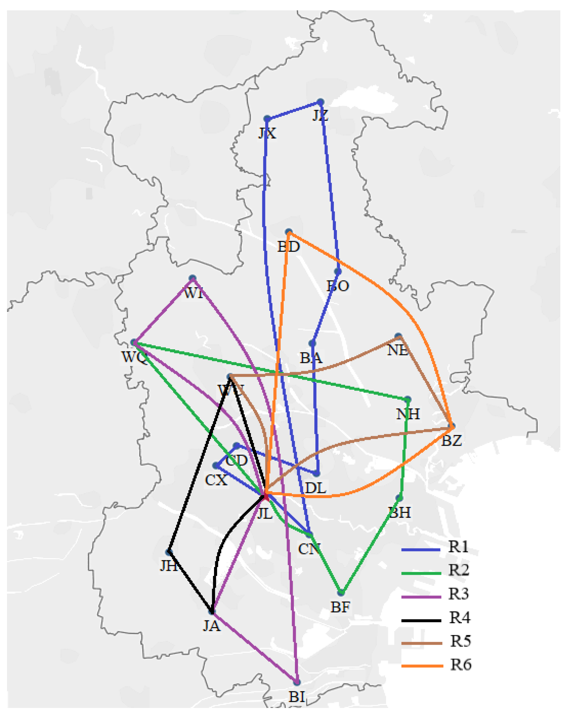
We utilized the hybrid ant colony-genetic algorithm to solve the model. We coded the hybrid ant colony-genetic algorithm in Matlab 2016b and implemented it on a personal computer with a 1.70 GHz i5 processor, 8 GB of RAM, and the Windows 10 operating system. The algorithm was set to terminate at the 1000th generation and executed 10 times. We chose the best solution from the 10 results. The best results for the CTSDVRP model and the two basic models are presented in Table 6, Table 7 and Table 8. The routes are listed in blue, green, purple, black, brown, and orange and correspond to the results in Figure 6, Figure 7 and Figure 8.

Table 6. The best results for the CTSDVRP model.

l	Route ID	Distribution Cost	The Customer Waiting Time	Weighted Customer Waiting Time
1	R1	389.18	47.21	40.36
2	R2	316.29	48.03	44.93
3	R3	353.6	60.57	55.66
4	R4	237.94	49.78	47.1
5	R5	258.62	64.11	58.49
6	R6	290.75	41.15	37.51
Total		1846.38	310.85	284.05

Table 7. The best results for Basic Model 1.

l	Route ID	Distribution Cost	The Customer Waiting Time	Weighted Customer Waiting Time
1	R1	392.36	47.22	40.4
2	R2	270.01	47.54	45.55
3	R3	308.05	57.97	53.26
4	R4	242.71	50.85	50.32
5	R5	341.02	66.02	62.4
6	R6	235.59	39.13	36.54
Total		1789.73	308.72	288.47

Note: For Basic Model 1, the customer satisfaction is described by the actual customer waiting time, and the weighted customer waiting time is not generated. To better illustrate the effectiveness of the CTSDVRP model, we calculated the weighted waiting time for the best solution, and this weighted waiting time is measured by the quantity of the end product produced by the corresponding delivery quantities of the two products.

Table 8. The best results for Basic Model 2.

l	Route ID	Distribution Cost	The Customer Waiting Time	Weighted Customer Waiting Time
1	R1	395.93	48.87	41.85
2	R2	325.26	50.45	46.84
3	R3	224.92	54.16	52.64
4	R4	318.45	77.45	71.03
5	R5	285.96	39.63	35.55
6	R6	252.28	39.49	36.72
Total		1802.8	310.04	284.63

Note: For Basic Model 2, the weighted customer waiting time is measured by the total quantity of the two products. To better illustrate the effectiveness of the CTSDVRP model, as in Basic Model 1, the weighted waiting time is also calculated based on the quantity of the end product produced by the corresponding delivery quantities of the two products.

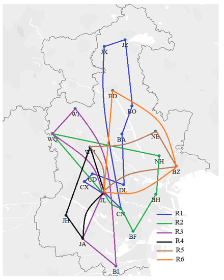
Figure 6. The CTSDVRP model routes.

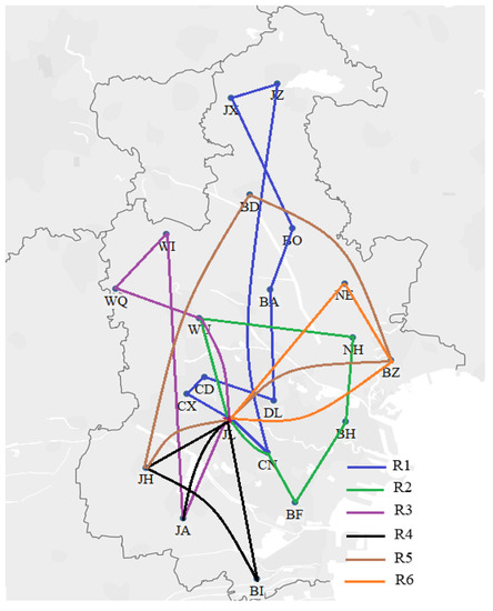
Figure 7. Basic Model 1 routes.

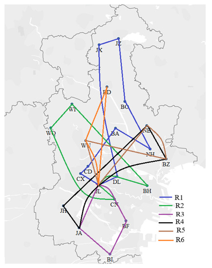
Figure 8. Basic Model 2 routes.

As shown in Figure 6, Figure 7 and Figure 8, the route ID refers to one vehicle, and there are six vehicles to perform delivery tasks. Many delivery routes change considerably in the different models. Note that instead of sending six cars at the same time, one car is sent immediately when a production cycle is finished. This means that the served time of all customers in the lth delivery is earlier than that of all customers in the $(l+1)$ th delivery. For example, in the CTSDVRP model, the demand of customer WQ was split into two deliveries, which were first served by route R2 (the green route) and then served by route R3 (the purple route).

In reality, the company has only 20 customers. To illustrate the effectiveness of the customized hybrid algorithm, based on the practical existing 20 customer nodes, we added 20, 40, and 60 nodes, respectively. These additional node locations were randomly selected on the city map. The demand for each additional 20 nodes is equal to the demand of practical existing 20 customer nodes. We coded the GA, ACO, and the hybrid ant colony-genetic algorithm in Matlab 2016b, respectively. Table 9 displays the results from the three algorithms.

Table 9. Comparison of the algorithms’ best solutions for the 20, 40, 60, and 80 nodes.

Number of Nodes	Algorithm	${\mathit{Y}}_{\mathit{best}}$	$\mathit{Wt}$	$\mathit{Rt}$	$\mathit{Cd}$	CPU (s)
20	Hybrid algorithm	10,886.32	310.85	284.05	1846.38	21.74
	GA	10,933.70	311.51	285.19	1931.69	20.12
	ACO	12,633.82	364.94	329.57	2204.81	30.08
40	Hybrid algorithm	38,145.69	1070.61	1000.03	2890.74	51.06
	GA	38,214.76	1072.73	1001.81	2918.01	54.71
	ACO	46,738.13	1333.73	1224.76	3947.14	70.45
60	Hybrid algorithm	83,674.52	2321.58	2195.66	4790.83	98.22
	GA	83,950.39	2333.17	2202.79	4886.56	93.95
	ACO	103,864.80	2936.20	2725.48	5929.60	125.60
80	Hybrid algorithm	147,413.81	4068.87	3869.89	7158.80	147.73
	GA	147,774.65	4084.30	3879.23	7280.61	133.64
	ACO	185,568.16	5456.41	4872.71	8104.85	189.62

In Table 9, the columns headed with $Y_{best}$, $Wt$, $Rt$, $Cd$, and CPU (s) indicate the objective function value, total actual customer waiting time, total weighted customer waiting time (based on the targeted service rate of the end products), total distribution cost, and the CPU time, respectively. As can be seen from Table 9, the hybrid algorithm shows a good performance in terms of a smaller objective function value, shorter total actual customer waiting time, smaller total weighted customer waiting time, and lower total distribution cost.

From the best solutions of the CTSDVRP model and the two basic models, we can draw some notable results:

Result 1.

Both the CTSDVRP model and Basic Model 2 can improve customer satisfaction.

We compared the total actual customer waiting time, total weighted customer waiting time, and total distribution costs of these three models. For Basic Model 1, although the total actual customer waiting time and total distribution cost are less than that for the CTSDVRP model and Basic Model 2, the total weighted customer waiting time is larger. Compared to Basic Model 1, the total actual customer waiting time in the CTSDVRP model increased by 2.13 h, and the total weighted customer waiting time decreased by 4.42 h. Compared to Basic Model 1, the total actual customer waiting time in Basic Model 2 increased by 1.32 h, and the total weighted customer waiting time decreased by 3.84 h. In summary, the CTSDVRP model and Basic Model 2 can effectively decrease the total weighted customer waiting time. This means that both the CTSDVRP model and Basic Model 2 can improve customer satisfaction.

Result 2.

The CTSDVRP model can improve customer satisfaction more effectively than Basic Model 2.

We examined which of the models improved customer satisfaction the most by analyzing the received quantities of A and B and the targeted service rate on the first receipt for customers whose demands were split into two deliveries. The analysis results from the CTSDVRP model and the two basic models are shown in Table 10, Table 11 and Table 12, respectively. The CTSDVRP model has the highest average targeted service rate (72.62%), followed by Basic Model 2 (49.60%) and Basic Model 1 (36.41%). Therefore, both the CTSDVRP model and Basic Model 2 can improve customer satisfaction. Furthermore, in Basic Model 2, the targeted service rate on the first receipt for customer BZ is 2.11%, and the targeted service rate on the first receipt for customer DL and customer CN are less than 45%. In addition, from Table 6, Table 7 and Table 8, we observed that the total weighted customer waiting time of the CTSDVRP model is the smallest. This explains why the CTSDVRP model can improve customer satisfaction more effectively than Basic Model 2.

Table 10. The delivery result of customers whose demands were split in the CTSDVRP model.

Customer ID	Received Quantity for the First Time		Targeted Service Rate	Received Quantity for the Second Time		Cumulative Service Rate
	A	B		A	B
CN	98	64	52.86%	77	65	100%
WQ	245	119	85.16%	12	23	100%
JA	441	156	92.59%	35	0	100%
WU	443	222	73.43%	215	49	100%
BZ	386	193	59.04%	272	132	100%

Table 11. The delivery result of customers whose demands were split in Basic Model 1.

Customer ID	Received Quantity for the First Time		Targeted Service Rate	Received Quantity for the Second Time		Cumulative Service Rate
	A	B		A	B
CN	98	64	52.86%	77	65	100%
WQ	245	119	43.91%	413	152	100%
JA	62	52	14.81%	414	104	100%
WU	307	229	61.15%	215	49	100%
BZ	57	83	9.34%	601	242	100%

Table 12. The delivery result of customers whose demands were split in the Basic Model 2.

Customer ID	Received Quantity for the First Time		Targeted Service Rate	Received Quantity for the Second Time		Cumulative Service Rate
	A	B		A	B
DL	5	43	20%	130	7	100%
CN	156	51	44.29%	19	78	100%
JA	441	156	92.59%	35	0	100%
NE	399	222	87.32%	0	36	100%
BZ	44	0	2.11%	614	325	100%
WU	386	139	51.29%	272	132	100%

Result 3.

The distribution scheme for the CTSDVRP model may be the best choice for managers.

Compared to Basic Model 1, the weighted customer waiting time of the CTSDVRP model and Basic Model 2 decreased by 1.53% and 1.33%, and the average targeted service rate of the CTSDVRP model and Basic Model 2 increased by 99.45% and 36.23%. This also illustrates that the CTSDVRP model can improve customer satisfaction more effectively than Basic Model 2. However, the total distribution cost of the CTSDVRP model and Basic Model 2 simultaneously increased by 0.73% and 3.17%. This means that the improvement of customer satisfaction is at the expense of distribution costs. From Table 6, Table 7 and Table 8, we observed that the total distribution costs of the CTSDVRP model is only 3.33% higher than that of Basic Model 2. This means that the CTSDVRP model can effectively improve customer satisfaction with a minimal distribution cost increase. Therefore, managers are most likely to prefer the CTSDVRP model.

5.3. Sensitivity Analysis

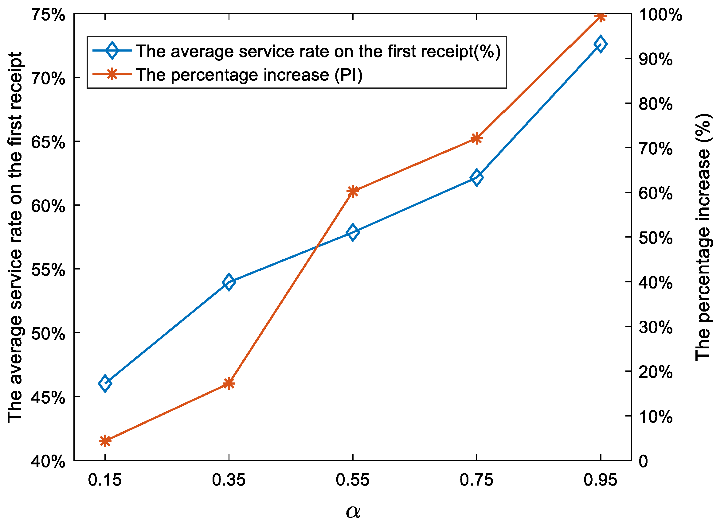
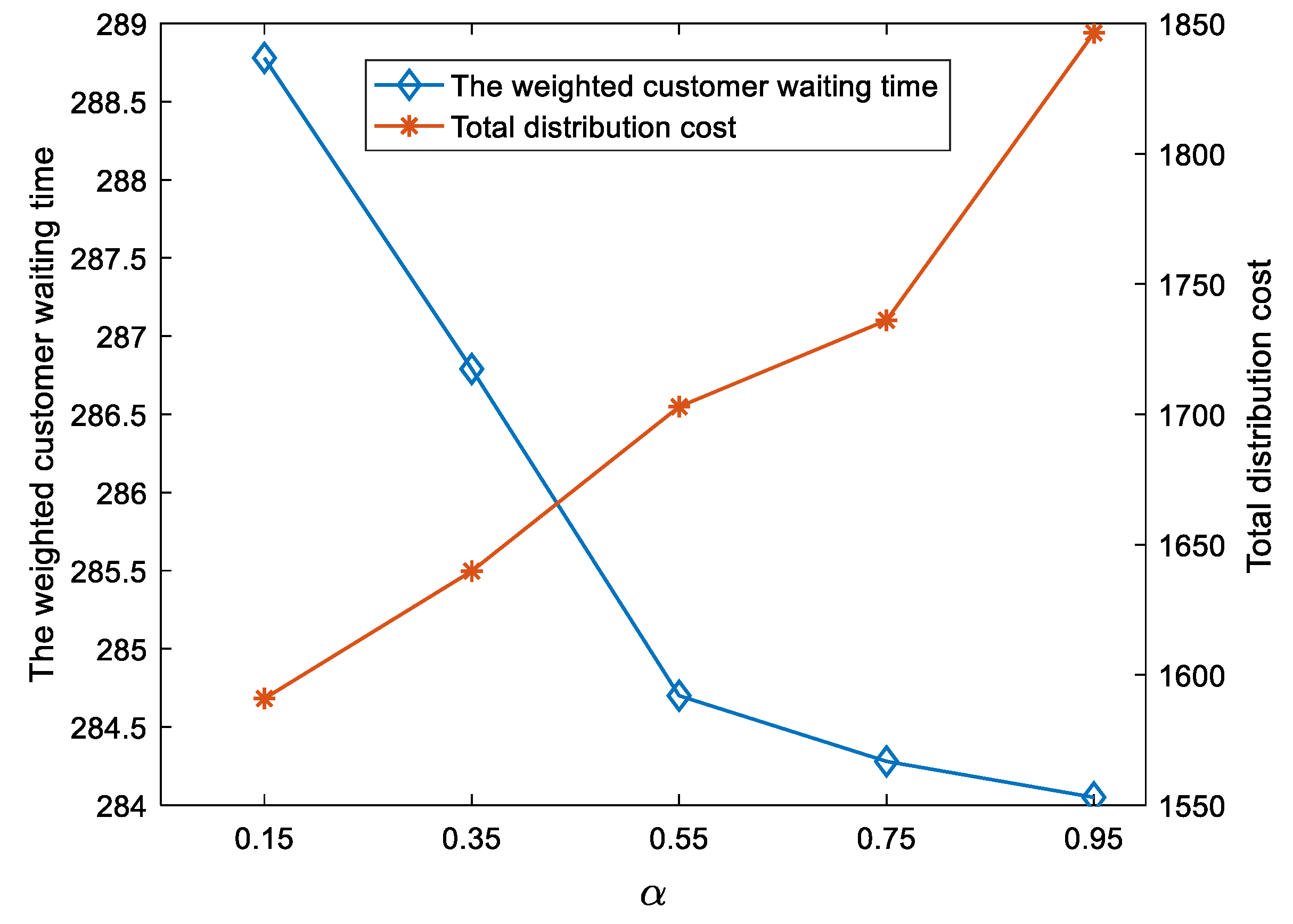
To further illustrate that the CTSDVRP model can effectively improve customer satisfaction, we analyzed the impacts of the $\alpha$ values on the total weighted customer waiting time, total distribution costs, and the average targeted service rate on the first receipt for customers whose demands were split. To measure the percentage increase (PI) of the average targeted service rate on the first receipt for the CTSDVRP model compared to that for Basic Model 1, the PI was introduced to evaluate the performance of the average targeted service rate on the first receipt. The PI is calculated in Equation (22):

$$\mathrm{PI}=\frac{\mathrm{The}\mathrm{average}\mathrm{service}\mathrm{rate}\mathrm{for}\mathrm{the}\mathrm{CTSDVRP}\mathrm{model}-\mathrm{The}\mathrm{average}\mathrm{service}\mathrm{rate}\mathrm{for}\mathrm{Basic}\mathrm{Model}1}{\mathrm{The}\mathrm{average}\mathrm{service}\mathrm{rate}\mathrm{for}\mathrm{Basic}\mathrm{Model}1}$$

(22)

For selected $\alpha$ values (0.15, 0.35, 0.55, 0.75, 0.95), we fixed the other parameters, and the results are shown in Figure 9 and Figure 10. Some results can be drawn as follows.

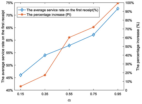
Figure 9. Impacts of $\alpha$ on the average service rate on the first receipt.

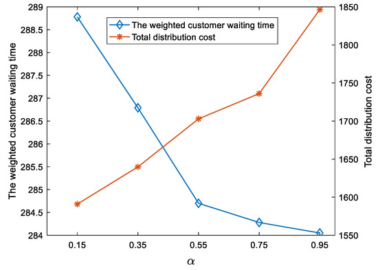
Figure 10. Impacts of $\alpha$ on total weighted customer waiting time and total distribution cost.

Result 4.

As managers focus more on customer satisfaction, the CTSDVRP model increases the average targeted service rate more substantially than Basic Model 1.

The average targeted service rate on the first receipt and the PI greatly changes as $\alpha$ increases, as shown in Figure 9. As $\alpha$ increases from 0.15 to 0.95, the average targeted service rate on the first receipt increases from 46.03% to 72.62%, and the PI increases from 4.37% to 99.43%. Therefore, as managers pay more and more attention to customer satisfaction, the CTSDVRP model increases the average targeted service rate more substantially than Basic Model 1. The reason for the change in the results is mainly because Basic Model 1 does not consider the production efficiency on the customer side during delivery.

Result 5.

For the CTSDVRP model, the improvement of customer satisfaction is at the expense of increased distribution costs.

As shown in Figure 10, the total weighted customer waiting time greatly decreases as $\alpha$ increases from 0.15 to 0.55 and slightly decreases as $\alpha$ increases from 0.55 to 0.95. The distribution cost increases from 1590.91 to 1846.38 as $\alpha$ increases from 0.15 to 0.95. This illustrates that the improvement of customer satisfaction is at the expense of increasing total distribution costs. For managers, this is an unavoidable tradeoff. Therefore, managers can choose the appropriate $\alpha$ values according to their preferences.

6. Conclusions

In this paper, we addressed a two-product distribution problem for State Grid in China. We modeled this problem as a customer-centric, two-product split delivery vehicle routing problem (CTSDVRP). Two decisions were made for solving this problem: the routing of the vehicles and the quantities of the two products in each delivery. Given the unique characteristics of this problem, we considered the weighted customer waiting time in customer satisfaction.

We presented three different models: Basic Model 1, Basic Model 2, and the CTSDVRP model. In Basic Model 1, the customer satisfaction is described by the actual customer waiting time. Different from Basic Model 1, customer satisfaction in the Basic Model 2 and the CTSDVRP model is described by the weighted customer waiting time. In Basic Model 2, the weighted customer waiting time is measured by the total delivery quantities of Product 1 and Product 2. However, this weighted customer waiting time ignores the interdependency of the two products. We improved this weighted customer waiting time in the CTSDVRP model, which is measured by the quantities of the end product resulting from the two products. In order to solve the model, we proposed a customized hybrid ant colony-genetic optimization algorithm.

Furthermore, the general VRP model saves more costs for the company at the expense of customer satisfaction. This trade-off must be carefully balanced by the decision-makers for the company’s and the customers’ concerns. Our numerical results demonstrate that the CTSDVRP model can increase the average targeted service rate on the first receipt, so customers can convert the received parts into more final products. Therefore, the best solution of the CTSDVRP model is the best choice for companies because it can effectively improve customer satisfaction. Moreover, managers should fully investigate customers’ time values to provide a buffer for the delivery time to save costs. In addition, we found that the weight of customer satisfaction had a significant impact on the total weighted customer waiting time, total distribution costs, and average targeted service rate on the first receipt. Thus, decision-makers should carefully choose the appropriate $\alpha$ values based on the company’s preferences.

Future research may extend the CTSDVRP model for a heterogeneous fleet. This study is based on a homogeneous fleet setting in which each vehicle has the same capacity. However, vehicle capacities may differ in real life. Note that in State Grid’s case, the vehicle capacity determines the verification quantities of the two products in each production cycle. Inspired by that, we would like to add heterogeneous fleet constraints to the CTSDVRP model in a future paper.

References

- CEO Says Volkswagen Has ‘Seen the Worst’ of the Chip Shortage. Available online: https://edition.cnn.com/2021/10/28/cars/volkswagen-chip-shortage/index.html (accessed on 28 October 2021).
- Manufacturing PMI® at 60.8%. Available online: https://www.ismworld.org/supply-management-news-and-reports/reports/ism-report-onbusiness/pmi/october/ (accessed on 1 November 2021).
- Rieck, J.; Ehrenberg, C.; Zimmermann, J. Many-to-many location-routing with inter-hub transport and multi-commodity pickup-and-delivery. Eur. J. Oper. Res. 2014, 236, 863–878. [Google Scholar] [CrossRef]
- Martínez-Salazar, I.; Angel-Bello, F.; Alvarez, A. A customer-centric routing problem with multiple trips of a single vehicle. J. Oper. Res. Soc. 2015, 66, 1312–1323. [Google Scholar] [CrossRef]
- Moshref-Javadi, M.; Lee, S. The customer-centric, multi-commodity vehicle routing problem with split delivery. Exp. Syst. Appl. 2016, 56, 335–348. [Google Scholar] [CrossRef]
- Oltra-Badenes, R.; Gil-Gomez, H.; Guerola-Navarro, V.; Vicedo, P. Is It Possible to Manage the Product Recovery Processes in an ERP? Analysis of Functional Needs. Sustainability 2019, 11, 4380. [Google Scholar] [CrossRef] [Green Version]
- Dror, M.; Trudeau, P. Savings by Split Delivery Routing. Transp. Sci. 1989, 23, 141–145. [Google Scholar] [CrossRef]
- Archetti, C.; Speranza, M.G. Vehicle routing problems with split deliveries. Int. Trans. Oper. Res. 2012, 19, 3–22. [Google Scholar] [CrossRef]
- Ho, S.; Haugland, D. A tabu search heuristic for the vehicle routing problem with time windows and split deliveries. Comput. Oper. Res. 2004, 31, 1947–1964. [Google Scholar] [CrossRef]
- Salani, M.; Vacca, I. Branch and price for the vehicle routing problem with discrete split deliveries and time windows. Eur. J. Oper. Res. 2011, 213, 470–477. [Google Scholar] [CrossRef] [Green Version]
- Luo, Z.; Qin, H.; Zhu, W.; Lim, A. Branch and price and cut for the split-delivery vehicle routing problem with time windows and linear weight related cost. Transp. Sci. 2016, 51, 668–687. [Google Scholar] [CrossRef]
- Khodabandeh, E.; Bai, L.; Heragu, S.S.; Evans, G.W.; Elrod, T.; Shirkness, M. Modelling and solution of a large-scale vehicle routing problem at GE appliances and lighting. Int. J. Prod. Res. 2017, 55, 1100–1116. [Google Scholar] [CrossRef]
- Fu, Z.; Liu, W.; Qiu, M. A Tabu Search Algorithm for the Vehicle Routing Problem with Soft Time Windows and Split Deliveries by Order. Chin. J. Manag. Sci. 2017, 25, 78–86. [Google Scholar]
- Li, J.; Qin, H.; Baldacci, R.; Zhu, W. Branch-and-price-and-cut for the synchronized vehicle routing problem with split delivery, proportional service time and multiple time windows. Transp. Res. Part E Logist. Transp. Rev. 2020, 140, 101955. [Google Scholar] [CrossRef]
- Lwspay, H.; Suchan, K. A case study of consistent vehicle routing problem with time windows. Int. Trans. Oper. Res. 2021, 28, 1135–1163. [Google Scholar] [CrossRef]
- Chan, F.T.S.; Shekhar, P.; Tiwari, M.K. Dynamic scheduling of oil tankers with splitting of cargo at pickup and delivery locations: A Multi-objective Ant Colony-based approach. Int. J. Prod. Res. 2014, 52, 7436–7453. [Google Scholar] [CrossRef]
- Qiu, M.; Fu, Z.; Eglese, R.; Tang, Q. A Tabu Search algorithm for the vehicle routing problem with discrete split deliveries and pickups. Comput. Oper. Res. 2018, 100, 102–116. [Google Scholar] [CrossRef] [Green Version]
- Gschwind, T.; Bianchessi, N.; Irnich, S. Stabilized branch-price-and-cut for the commodity-constrained split delivery vehicle routing problem. Eur. J. Oper. Res. 2019, 278, 91–104. [Google Scholar] [CrossRef] [Green Version]
- Fazi, S.; Fransoo, J.C.; Woensel, T.V.; Dong, J.X. A variant of the split vehicle routing problem with simultaneous deliveries and pickups for inland container shipping in dry-port based systems. Transp. Res. Part E Logist. Transp. Rev. 2020, 142, 102057. [Google Scholar] [CrossRef]
- Wolnger, D.; Salazar-Gonzalez, J. The Pickup and Delivery Problem with Split Loads and Transshipments: A Branch-and-Cut Solution Approach. Eur. J. Oper. Res. 2021, 289, 470–484. [Google Scholar] [CrossRef]
- Zhang, Z.; Cheang, B.; Li, C.; Lim, A. Multi-commodity demand fulfillment via simultaneous pickup and delivery for a fast fashion retailer. Comput. Oper. Res. 2019, 103, 81–96. [Google Scholar] [CrossRef]
- Tavakkoli-Moghaddam, R.; Safaei, N.; Kah, M.; Rabbani, M. A New Capacitated Vehicle Routing Problem with Split Service for Minimizing Fleet Cost by Simulated Annealing. J. Frankl. Inst. 2007, 344, 406–425. [Google Scholar] [CrossRef]
- Belfioreab, P.; Yoshizaki, H. Scatter search for a real-life heterogeneous fleet vehicle routing problem with time windows and split deliveries in Brazil. Eur. J. Oper. Res. 2009, 199, 750–758. [Google Scholar] [CrossRef]
- Hertz, A.; Uldry, M.; Widmer, M. Integer linear programming models for a cement delivery problem. Eur. J. Oper. Res. 2012, 222, 623–631. [Google Scholar] [CrossRef]
- Yousefikhoshbakht, M.; Didehvar, F.; Rahmati, F. Solving the heterogeneous fixed fleet open vehicle routing problem by a combined metaheuristic algorithm. Int. J. Prod. Res. 2014, 52, 2565–2575. [Google Scholar] [CrossRef]
- Wang, L.; Kinable, J.; Woensel, T. The fuel replenishment problem: A split-delivery multi-compartment vehicle routing problem with multiple trips. Comput. Oper. Res. 2021, 118, 104904. [Google Scholar] [CrossRef]
- Gulczynski, D.; Golden, B.; Wasil, E. The split delivery vehicle routing problem with minimum delivery amounts. Transp. Res. Part E Logist. Transp. Rev. 2010, 46, 612–626. [Google Scholar] [CrossRef]
- Han, F.; Chu, Y. A multi-start heuristic approach for the split-delivery vehicle routing problem with minimum delivery amounts. Transp. Res. Part E Logist. Transp. Rev. 2016, 88, 11–31. [Google Scholar] [CrossRef]
- Xiong, Y.; Gulczynski, D.; Kleitman, D.; Golden, B.; Wasil, E. A worst-case analysis for the split delivery vehicle routing problem with minimum delivery amounts. Optim. Lett. 2013, 7, 1597–1609. [Google Scholar] [CrossRef]
- Nucamendi, S.; Cardona-Valdes, Y.; Acosta, A. Minimizing customer’s waiting time in a vehicle routing problem with unit demands. J. Comput. Syst. Sci. Int. 2015, 54, 866–881. [Google Scholar] [CrossRef]
- Huang, Y.; Yang, Q.; Li, Q.; Zhang, W. The delivery vehicle scheduling considering agents’ perception satisfaction toward waiting time. Ind. Eng. J. 2017, 4, 35–40. [Google Scholar]
- Wu, B.; Shao, J.; Fang, Y. Research on open vehicle routing problem based on satisfaction of customers. Comput. Eng. 2009, 35, 193–194. [Google Scholar]
- Fan, J. The vehicle routing problem with simultaneous pickup and delivery considering customer satisfaction. Oper. Res. Manag. Sci. 2011, 20, 60–64. [Google Scholar]
- Zhang, H.; Zhang, Q.; Ma, L.; Zhang, Z. A hybrid ant colony optimization algorithm for a multi-objective vehicle routing problem with flexible time windows. Inform. Sci. 2019, 490, 166–190. [Google Scholar] [CrossRef]
- Yu, J.; Cheng, W.; Wu, Y. Path planning of fresh takeout considering customer satisfaction. Ind. Eng. Manag. 2021, 26, 158–167. [Google Scholar]
- Chen, J.; Fan, T.; Pan, F. Urban delivery of fresh products with total deterioration value. Int. J. Prod. Res. 2021, 7, 2218–2228. [Google Scholar] [CrossRef]
- Luan, J.; Yao, Z.; Zhao, F.; Song, X. A novel method to solve supplier selection problem: Hybrid algorithm of genetic algorithm and ant colony optimization. Math. Comput. Simulat. 2019, 156, 294–309. [Google Scholar] [CrossRef]
- Peng, P.; Zhang, G. Improvement and simulation of ant colony algorithm based on genetic gene. Comput. Eng. Appl. 2010, 46, 43–45. [Google Scholar]
Publisher’s Note: MDPI stays neutral with regard to jurisdictional claims in published maps and institutional affiliations. |
© 2022 by the authors. Licensee MDPI, Basel, Switzerland. This article is an open access article distributed under the terms and conditions of the Creative Commons Attribution (CC BY) license (https://creativecommons.org/licenses/by/4.0/).