Abstract
The performance and stability of the transonic fan stage with a nonuniform inflow is a key issue in aero engine operation, and the coupling of inlet distortion and low Reynolds numbers at high altitude creates more severe challenges to aero engines. This work used computational methods to explore the performance and stability of a transonic fan stage with inlet distortion and a low Reynolds number. To investigate this issue, the transonic fan stage NASA stage 67 with a 180° total pressure distortion at a low Reynolds number was selected as the test case. Full-annulus 3D unsteady simulations were conducted to reveal the details of the flow field under coupling conditions. The computational results under different conditions were analyzed and showed that the coupling effect was not linearly stacked with single factors. The low Reynolds number in the coupling case thickened the boundary layer on the blade surface, and, on the one hand, the profile loss in the hub region increased. On the other hand, the structure of shock wave was converted in the tip region, which increased the shock loss significantly. In addition, the variation in the shock wave structure reconstructed the pressure distribution on the blade surface, allowing the fluid to migrate to the tip region, which affected the tip flow structure and ultimately delayed the stability boundary.
1. Introduction
Inlet distortion is one of the inevitable phenomena during the operation of aero engine compression systems. Flight maneuvers, crosswinds, and other issues can lead to a nonuniform inlet airflow. Distortion deteriorates the performance of the compressor and consumes the available surge margin, raising the risk to the whole engine operation. Numerous studies have attempted to explore the effects of distortion on the performance and stability of the compressor. Decades ago, researchers tried to investigate the relationship between inlet distortion and compressor performance and stability experimentally [1,2,3,4,5] Longley et al. [6,7] tested the effects of rotational inlet distortion on a multistage compressor and found that the degradation in stability margin is immensely related to the velocity of flow nonuniformity propagation around the annulus. In recent years, Gunn et al. [8], Rademakers et al. [9], and Naseri et al. [10] investigated the effect of inlet distortion on the performance and stability of compressors experimentally. The results of tests showed the quantitative relationship of inlet distortion and compressor stability margin. Furthermore, Perovic et al. [11] explored the stall inception in a Boundary Layer Ingesting (BLI) fan. However, experimental testing can be time-consuming and costly, and the test data available from testing are somewhat limited. With the development of computer technology, Computational Fluid Dynamics (CFD) provides a more economical and reliable method. Fidalgo et al. [12] investigated the propagation process of stagnation pressure circumferential distortion inside the compressor by means of high-fidelity simulations. Zhang and Vahdati [13,14,15] carried out unsteady simulations to study the influence of total pressure distortion on the loss of stall margin, and the results showed that when the speed decreased, the tip leakage flow oscillated periodically and the stall margin loss further increased. Additionally, Zhang and Vahdati [16] studied the stall and recovery process of a transonic fan with and without distortion. In their study, the stall behavior of the fan was changed with the presence of inlet distortion, and the number of stall cells was reduced from six to only one. Ma et al. [17] conducted mixed-fidelity numerical research for the interaction of fan-distortion, and the results showed that the fan had a significant effect in reducing distortions. It can be seen that the numerical simulation has become an efficient and accurate method to study the effects of inlet distortion in compressors. However, distortion as one of the destabilizing factors usually does not present alone. Typically, it is necessary to consider the effect of low Reynolds numbers on the aero engine when the aircraft is flying at a high altitude.
The previous researchers have attempted to figure out and assess the coupling effects of distortion and Reynolds number via experiments. Wallner et al. [18] carried out detailed research on the effects of inlet distortion on the J75-P-1 turbojet engine stall characteristics and operating limits in the Lewis altitude wind tunnel. Moreover, the effect of different forms of distortion profiles on performance was studied and data were obtained over a range of compressor speeds at an altitude of 50,000 ft and a flight Mach number of 0.8. Cousins et al. [19] conducted altitude testing of inlet distortion on the T800 engine to examine the effects of temperature and pressure distortion on the surge margin of the compression system at various altitudes, and the temperature and pressure distortion were generated by classical screens and a hydrogen burner system, respectively. The results showed that combined temperature and pressure distortion affect the stability in different ways depending on the screen orientation and altitude, but in general, had a small effect on stability. Lee et al. [20] carried out preliminary testing to evaluate the operational capability of three different types of distortion-simulating devices in the Altitude Engine Test Facility (AETF) and observed the deterioration in overall gas turbine engine performance and stability. It can be indicated that efforts have been made to obtain a series of data for the distortion tests in altitude test equipment, but due to the cost and complexity of the engine altitude test, the coupling effects still need further investigation for accurate assessment of compressor aerodynamic stability. As for the coupled simulations of Reynolds number and inlet distortion, there is no relevant research seen currently.
Therefore, this paper sets out to (1) investigate the performance of the compressor within inlet distortion and low Reynolds numbers using CFD, (2) analyze the sources and composition of losses in the compressor under the coupling condition, and (3) explain the difference of TLF (tip leakage flow) under distortion and coupling conditions and the influence on the stability boundary.
The following part of this paper is organized as follows: the computational setups for 3D full-annulus steady/unsteady simulations are introduced in Section 2, which includes the research subject, numerical methods, and validations. Then, in Section 3, the problem descriptions are proposed. Next, the coupling effects on the overall aerodynamic performance of the compressor are analyzed in Section 4. The sources and composition of the losses are demonstrated in detail, which is followed by the comparison of tip region flows within distortion and coupling conditions. Finally, the main findings in this paper are concluded in Section 5.
2. Computational Setups
2.1. Research Subject
The case selected in this work is the NASA rotor 67 transonic axial-flow fan stage, as presented in Figure 1. On the one hand, the experimental data of this fan stage are sufficient and publicly available. On the other hand, NASA stage 67 is a typical transonic fan stage and is widely accepted by researchers. This fan is designed by NASA Lewis Research Center [21]. The experiments were carried out at the W8 Single Stage Compressor Test Facility [22] at NASA Glenn Research Centre. The single-stage calculation model used for the following study consists of a rotor row with 22 blades and a stator row (S67A) with 34 blades. At the design condition, the rotational speed is 16,043 rpm. The corrected mass flow and total pressure ratio of the isolated rotor are 33.25 kg/s and 1.63, respectively, resulting in a tip relative Mach number of 1.38. Other characteristic parameters are presented in Table 1.
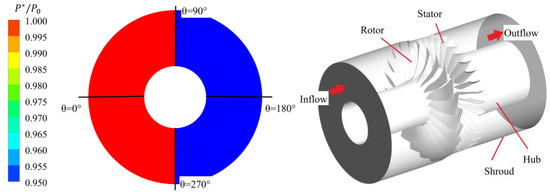
Figure 1.
Schematic of the computational domain and inlet pressure distortion profile.

Table 1.
NASA Rotor 67 main characteristic parameters at the design point.
2.2. Numerical Methods
The 3D hybrid combination of the finite volume method and finite element method CFD commercial solver, ANSYS CFX 18.2, is applied to compute the flow field in the transonic axial fan stage. Reynolds-Averaged Navier–Stokes (RANS) equations are selected to depict the conservation of mass, momentum, and energy of the air, and the two-equation turbulence model ( SST) with the transition model is used for calculating the effect of Reynolds number in this work.
To accurately predict the flow details under the coupling condition, Unsteady Reynolds-Averaged Navier–Stokes (URANS) simulations are used in the study. For the unsteady settings, the physical time step is set to , and the number of numerical iterations within a physical time-step is set to be 20. The calculations are converged when the pressure at the leading edge of rotor becomes periodic, and the error in mass flow at the inlet and outlet of the computational domain is less than 2%.
To study the coupling case of the circumferential total pressure distortion and low Reynolds numbers on the single-stage compressor performance, full-annulus calculations are applied. The computational domain is shown in Figure 1. In the setup of the computational domain, according to the Laplace equation, the inlet boundary is extended ~0.5 times the circumference of the casing upstream of the blade leading edge, and the outlet boundary is extended ~1.0 times the circumference of the casing downstream of the blade trailing edge. The uniform inlet boundary is an injection with uniform total temperature (288.15 K) and total pressure (101,325 Pa). The average static pressure is specified at the exit of the computational domain. Meanwhile, nonslip and adiabatic conditions are set on the hub, shroud, and blade parts.
For inlet distortion simulations, a low total pressure sector of 180° is placed at the inlet boundary (blue region in Figure 1). To evaluate the distortion intensity, DI is used and defined as:
where and represent the total pressure of the inlet distorted and clean sectors, respectively.
For calculations at low Reynolds numbers, inlet conditions are determined according to ISA (International Standard Atmosphere), and the transition model in the SST model is switched on. Meanwhile, RNI (Reynolds number index) is used to present the intensity of the Reynolds number. RNI is defined as the ratio of a high-altitude Reynolds number to sea-level Reynolds number.
where , , and are the air parameters at high altitude, and is the dynamic viscosity of the air at sea level.
The computational grid is generated by commercial software AutoGrid 5. A structured O4H-type grid topology is selected in each blade passage. As shown in Figure 2, the blade surface is surrounded by the O-grid, and the rest is divided into the H-grid. The mesh in the tip region is locally refined.
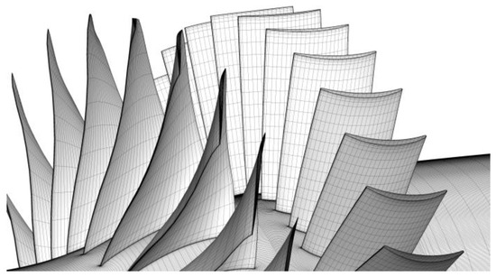
Figure 2.
Computational meshes for NASA Stage 67.
The meshes with the different numbers of nodes are calculated to determine mesh independence. The overall performances among the simulations with different nodes are compared in Figure 3. The normalize mcor in the legend stands for the ratio of corrected mass flow at operating point to the corrected mass flow at choke point. The red line (normalize mcor = 0.96) is the result near the peak efficiency point, and the black line (normalize mcor = 0.94) is that near the stall point. The total pressure ratio varies no more than 0.2% when the node number of the full circle exceeds . Based on the above analysis, the medium grid with nodes is sufficient for compressor performance calculations. The mesh distribution is 83 × 45 × 47 in the streamwise, blade-to-blade, and spanwise directions, respectively, for the rotor domain. The normal size of the first cell near the wall is set to 1 µm, which represents that the normalized wall distance (y+) is less than 1 in most regions, and the maximum value is less than 1.5.
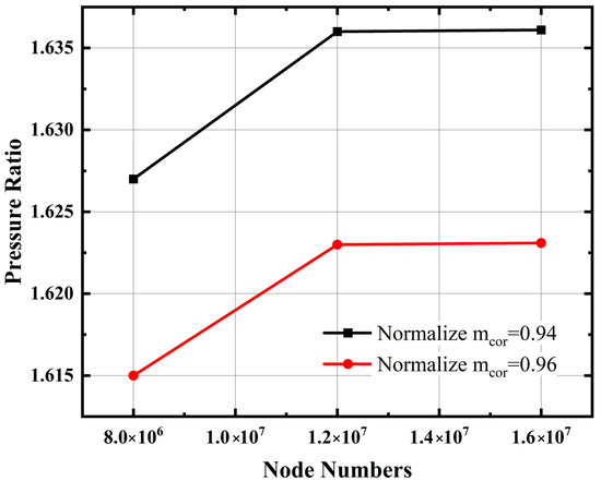
Figure 3.
Mesh independence study for NASA Stage 67.
2.3. Validations
To validate the numerical methods, the numerical results are compared with the experiment data [22]. Figure 4 shows the comparisons of CFD and test results. For the total pressure ratio of the compressor stage, due to the deformation of the compressor geometry in the rotating state, the curve of CFD is lower than the experimental data. The maximum deviation in mass flow is 0.5 kg/s, appearing at the choke point. The total pressure ratio deviation reaches a maximum of 0.04 at the choke point. The mean absolute percentage error (MAPE) of mass flow is about 1.1%, and total pressure ratio MAPE is 2.7%. There are two possible reasons for the deviations: (1) rotating parts deform in the test condition, which changes the original blade profile and tip clearance; (2) the test takes the rakes to measure the characteristics, while the simulations use mass flow average parameters to calculate the characteristics. In general, the results of numerical simulations agree well with the trend of experimental measurement points, and the discrepancy presented in this study is similar to other studies [23]. Therefore, the method is acceptable for the following studies.
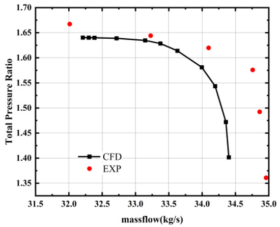
Figure 4.
Comparison of simulation and experimental results of NASA Stage 67.
To verify the ability of numerical methods in predicting flow field information, the radial distributions of key parameters near the peak efficiency (PE) point are compared with experimental data. In Figure 5, the radial profiles at the PE point for the total pressure ratio and total temperature ratio downstream of the single rotor are presented. Generally, the profiles match well with the experimental results. The results are normalized with (101,325 Pa) and (288.15 K). In Figure 5a, the predicted total pressure matches the trend of experimental data, except that it is slightly lower than the measuring value near the shroud. The maximum deviation is 0.04 at the 0.9 normalized spanwise location, and the MAPE is 1.4%. In Figure 5b, the predicted total temperature is in good agreement with the experimental data. The maximum deviation is 0.01 at the 0.9 normalized spanwise location, and the MAPE is 0.7%.
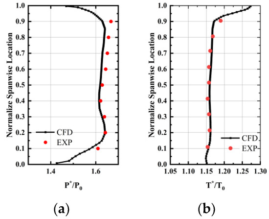
Figure 5.
Comparison of the radial distribution downstream of the rotor alone at PE. (a) Total pressure radial profile; (b) total temperature radial profile.
Furthermore, in order to verify the applicability of the transition model at low Reynolds numbers, a highly loaded turbine cascade Pak B is employed for validation [24,25,26]. Figure 6 presents the mesh topology of the cascade at mid-span, and the maximum normalized wall distance (y+) is less than 1. Figure 7 shows that the results predicted by the SST turbulence model with the transition model are in good agreement with the experimental data at . Compared with the SST model, the SST model with the transition model predicts the transition process of the blade suction surface, thus obtaining an accurate pressure coefficient distribution on the blade surface at low Reynolds numbers. The maximum deviation in near the transition point is 0.3, and the MAPE is 3%. Therefore, it shows that the present CFD model is proven to be accurate enough to acquire performances in the axial compressor at low Reynolds numbers, and it is used in the following simulations under the coupling condition.
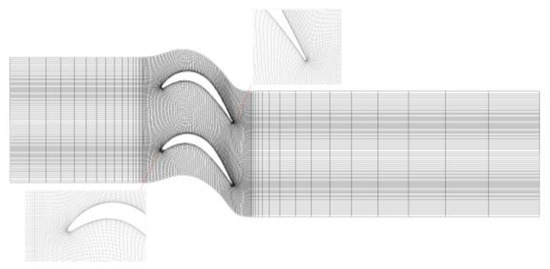
Figure 6.
Computational meshes for Pak B cascade.
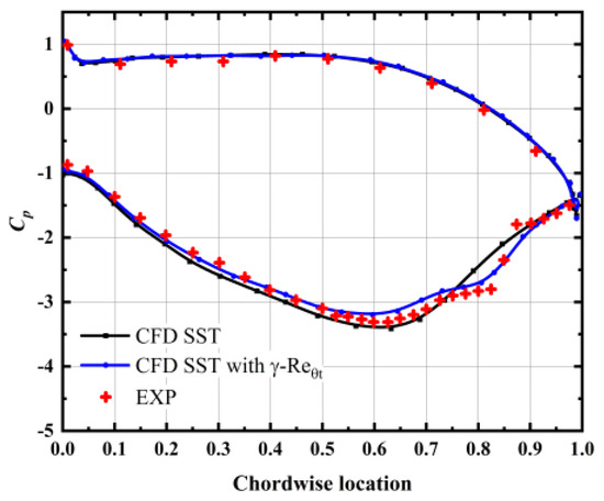
Figure 7.
Comparison of different numerical methods and experimental results at Re = 105.
Based on the validations mentioned above, the numerical methods in this work could make good predictions for the performance of the compressor. With the combination of steady and unsteady simulations, detailed flow field information can be obtained.
3. Problem Descriptions
The total pressure distortion leads to a nonuniform airflow to the compressor inlet, and the flow field of the blades passing through the distortion region deteriorates, which eventually results in the loss of aerodynamic performance. At low Reynolds numbers, the performance of the compressor also deteriorates significantly due to the enhanced viscous effects. In Figure 8, the compressor performances under different conditions are presented. The performance losses due to distortion are more pronounced under small mass flow rate conditions, while the losses induced by low Reynolds numbers is more significant under large mass flow rate conditions.
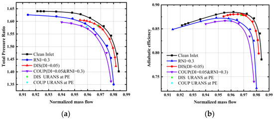
Figure 8.
Comparison of fan stage performances under different conditions. (a) Total pressure ratio characteristics; (b) adiabatic efficiency characteristics.
In Table 2, the performance losses are listed in different cases near the PE point. Compared with the uniform inlet airflow, the total pressure ratio and adiabatic efficiency are reduced with distorted inflow. The total pressure ratio decreases by 1.94% and the efficiency drops 0.45% in absolute value. Under the low Reynolds number condition, the performance of the compressor also decreases to a certain extent, the total pressure ratio reduces by 0.18% with little effect, and the efficiency drops by 1.19% in absolute value. For the coupling case, the losses in total pressure ratio and efficiency are 1.95% and 1.83%, respectively, not a linear stack related to losses under the single-factor conditions.
Table 2.
Comparison of performance losses under different working conditions (at PE point).
The star-shaped marker points in Figure 8 are the results of the unsteady calculations for the distortion and coupling cases, and the following analyses for losses and stability are mainly carried out on these two operating points. The definition of entropy loss coefficient is:
where and are the mass-averaged static temperature and velocity at the inlet, respectively. is defined as the change in entropy from rotor inlet to outlet. The radial distribution of entropy loss coefficients at the PE point obtained from URANS simulations is compared in Figure 9. The entropy loss coefficient in Figure 9 is the annulus mass-averaged value at different spanwise locations, and additional loss is defined by the following equation:
where is the entropy change under distortion or coupling conditions, and is the entropy change under the clean inlet condition. In the whole spanwise range, the additional loss under the coupling condition is no less than the additional loss under distortion. At 10% spanwise, the discrepancy between additional loss under coupling and distortion conditions is 0.019, with the largest difference of 0.11 in the tip region. It indicates that the coupling effects of the Reynolds number and inlet distortion on performance losses is mainly found in the low spanwise region near the hub and the tip region.
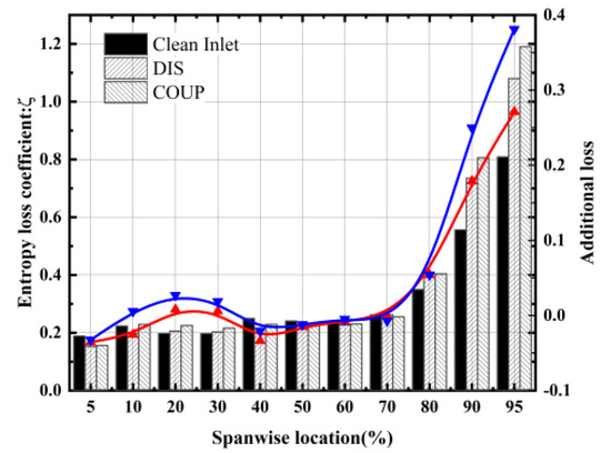
Figure 9.
Comparison of the entropy loss coefficient at different spanwise locations in various cases.
4. Results and Discussions
4.1. Nonuniform Flow Fields Upstream of the Rotor Blade Row
This section analyzes the difference in the flow field upstream of the fan stage when subjected to inlet distortion and coupling of distortion with low Reynolds numbers. Based on the results of the previous section, the flow analyses focus on the tip region. Figure 10 shows the time-averaged circumferential distribution of several critical aerodynamic parameters in the AIP section at the 95% spanwise location. Compared with the Ref. [12], although the distortion angle of the inflow is different, the distribution patterns of total pressure, static pressure, and axial velocity under the distortion condition are similar. However, the distribution of the aerodynamic parameters under the coupling condition changes. According to Figure 10a, in the upstream flow field from the inlet to AIP section, friction losses along the course cause a drop in the total pressure. In the coupling case of the inlet distortion and Reynolds number, the viscous loss of the upstream increases, and the total pressure drop is more significant. Figure 10b shows the static pressure distribution in the AIP section. The static pressure under the coupling case is higher than that under the inlet distortion condition. These finally lead to a circumferential distribution of axial velocity, as shown in Figure 10c. It can be noted that the overall axial velocity under the coupling condition is lower than that in the distortion case. On the one hand, this is due to the difference in the corrected mass flow rate at the PE point, and on the other hand, the relationship between the magnitude of the total pressure and static pressure makes the circumferential velocity with the coupling inflow smaller. Figure 10d depicts the comparison of the total pressure loss coefficient for the distortion and coupling conditions. The total pressure loss coefficient is defined as follows:
where represents the total pressure drop from the inlet of the computational domain to the AIP section. The denominator is the dynamic pressure at the inlet. In the circumferential location from 90° to 270°, the loss coefficient under the coupling condition is 0.0061 larger on average than that under the distortion condition. In the rest of the circumferential range, the loss coefficient under the coupling condition is higher than that under the distortion condition, about 0.0075. This indicates that the increase in upstream total pressure loss in the clean sector is slightly higher than that in the distortion sector with the coupling inflow.
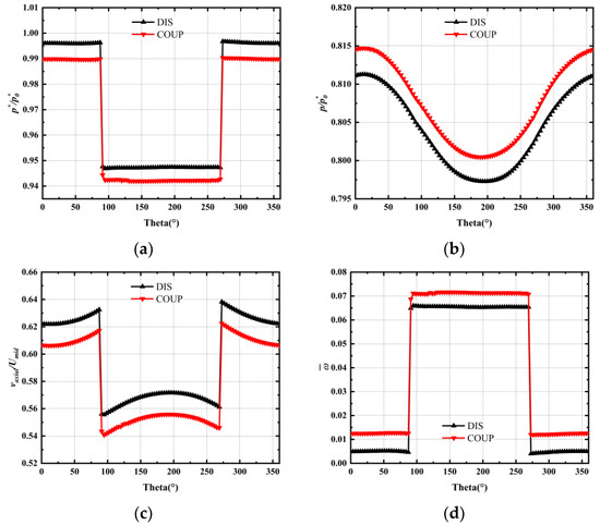
Figure 10.
Time-averaged, circumferential distributions of different parameters in the AIP section (at 95% spanwise). (a) Total pressure coefficient; (b) static pressure coefficient; (c) axial velocity coefficient; (d) loss coefficient.
Figure 11 shows the time-averaged circumferential distribution of swirl angle in the AIP section at the 95% spanwise location. According to the distribution pattern, there is a positive swirl in the circumferential location from 0 to 180 deg and a negative swirl in the circumferential location from 180° to 360°. The circumferential distribution of the swirl angle under the distortion and coupling conditions follows the same pattern and has similar values, with the largest discrepancy occurring at the junction of the distortion and clean regions. At 90° and 270° circumferential positions, the maximum value of the difference between the two conditions of swirl angle is about 0.15°. It demonstrates that the coupling inflow has less of an effect on the distribution of the airflow angle into the blade row, which means that the circumferential distribution of blade loading is the same in the two cases.
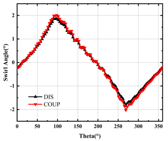
Figure 11.
Time-averaged, circumferential distributions of swirl angle in the AIP section (at 95% spanwise).
4.2. Loss Sources and Components under Coupling Condition
To find out the effects of inlet distortion and low Reynolds numbers on the performance loss of the compressor, this section mainly analyzes the sources, composition, and causes of the loss at different locations of the compressor. For loss assessment on a transonic fan stage, individual loss components consist of profile loss, shock loss, and secondary loss [27,28,29,30,31]. Considering the small effect of secondary loss near the PE point and the practice of approximating the sum of shock loss and profile loss as the total losses in Bloch’s study [32], the main focus in this study is on assessing profile loss and shock loss. Based on the distribution of additional losses in Section 3, the flow structures and loss analysis are mainly investigated for the 10% and 95% spanwise locations.
Figure 12 shows the circumferential distribution of entropy loss coefficient at the 10% spanwise location. The flow field comparison results in the clean sector and distorted sector are shown in Figure 13. In the full circumferential range, in the coupling case is higher than that under the inlet distortion condition. Comparing the flow field around the rotor blades under the two operating conditions, the wake of the rotor blades is enhanced under the coupling condition, and the wake enhancement is more significant in the distortion sector than in the clean sector. Figure 14 presents the zoomed-in results of the leading edge of the rotor blade in the distortion region, where the thickness of the displacement boundary layer on the blade suction surface increases by 13% at the 5% chord length location. It can be noted that the thickness of the boundary layer on the blade surface increases under the coupling condition. The low Reynolds number leads to an increase in the thickness of the boundary layer, and the friction loss within the boundary layer.
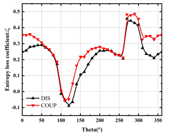
Figure 12.
Comparison of circumferential distribution of entropy loss coefficient at 10% spanwise.
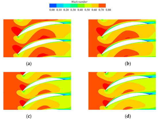
Figure 13.
Comparison of Mach number contours at 10% spanwise location. (a) Clean sector at DIS; (b) clean sector at COUP; (c) distortion sector at DIS; (d) distortion sector at COUP.
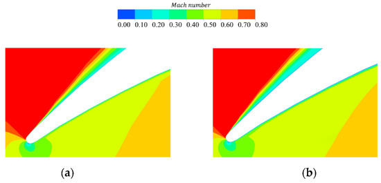
Figure 14.
Comparison of the zoomed-in view of Mach number contours at the rotor blade leading edge at 10% spanwise location. (a) DIS case; (b) COUP case.
At the 10% spanwise location, the flow is subsonic and the source of loss is mainly caused by the profile loss, which can be calculated in the following equation:
where is the boundary layer momentum thickness, is the chord length of the rotor blade, presents the boundary layer form factor, and and represent the air angle at the inlet and outlet of the blade row measured from the axial direction, respectively. The profile loss under the coupling condition is 0.037, and the profile loss within the distorted inflow is 0.033.
Figure 15 shows the circumferential distribution of at the 95% spanwise location. Though the under the coupling condition is also larger than that under the distortion condition, the causes of the losses are different. The Mach number contours of the distortion region are compared in Figure 16. Comparing the blade flow field under the two operating conditions, wake enhancement due to the coupling effect and thickened boundary layer both lead to the increase in the profile loss. In addition, the variation in the shock wave structure is also an important reason affecting losses. Figure 17 shows the schematic diagram of the variation in shock wave structure. Due to the low Reynolds number increasing the thickness of the boundary layer, the actual blade profile felt by the fluid changes, which affects the structure of the shock wave within the blade passage. The shock wave in the blade passage within the inlet distortion is an oblique shock wave, and the coupling effect increases the shock wave angle, more like a normal shock wave. The variation in the shock wave structure makes the shock wave loss increase significantly, and the shock loss in the tip region becomes a more important source of loss compared to the profile loss.
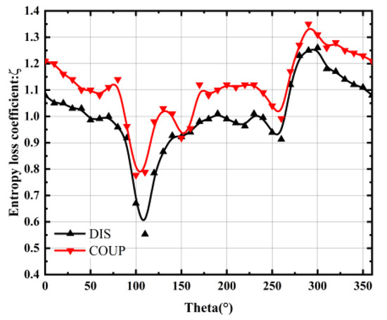
Figure 15.
Comparison of the circumferential distribution of entropy loss coefficient at 95% spanwise location.
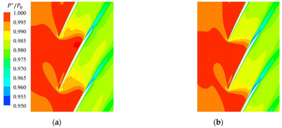
Figure 16.
Comparison of Mach number contours in distortion region at 95% spanwise location. (a) DIS case; (b) COUP case.
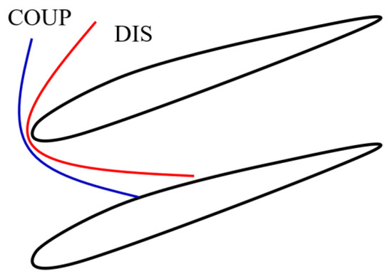
Figure 17.
Schematic diagram of the change in the structure of the shock wave.
According to the previous investigations, the efficiency drop in the transonic fan stage is predominantly determined by shock loss. Therefore, the shock loss has also naturally become a focus of attention in the transonic flow in the tip region, which can be expressed as:
where presents the blade angle of attack, and represents the minimum value of the angle of attack, which is the angle of attack at the PE point with clean inflow. The circumferential distribution of the shock loss in the tip region under these two conditions is shown in Figure 18. In the full circumferential range, the shock wave loss in the tip region in the coupling case is larger than the shock wave loss with distortion. Moreover, the shock wave loss reaches a maximum at the position of 90° and 270°, i.e., the junction of the distortion and clean regions.
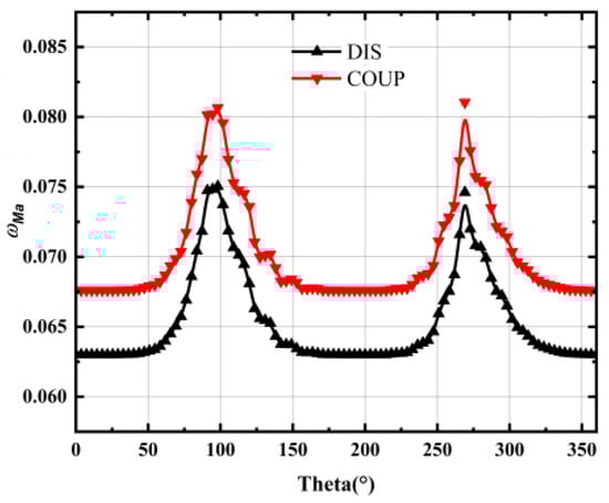
Figure 18.
Comparison of the circumferential distribution of shock loss.
4.3. Time Evolution of Blade Loading Distribution
The previous sections have analyzed the performance loss of the fan-stage and drawn a series of conclusions. To study the coupling effects on the stability boundary, this work focuses on the blade loading at different circumferential locations. Within a nonuniform inflow, the blade loading varies periodically during one revolution. This section aims to explore the load of a certain blade at different moments during one revolution. Figure 19 illustrates the key positions selected for analysis during the rotation of the blade in one revolution. The characteristics of the blade in the distortion region, the clean region, and the junction of the two regions are mainly studied. Figure 20 shows the blade loading distribution characteristics at different moments within one revolution under distortion and coupling conditions. The difference is mainly located in two points, one is the front half of the blade pressure surface and the other is the second half of the blade suction side. At different moments, the distribution of surface pressure on the blade pressure side is different. Under the coupling condition, the pressure distribution curve on the blade pressure side has a smaller slope than that under the distortion condition.
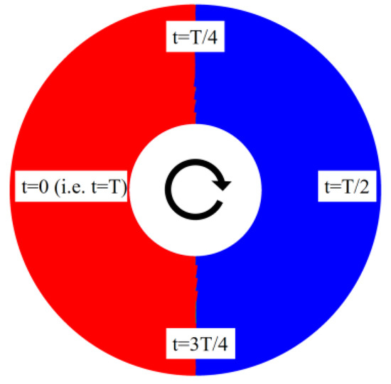
Figure 19.
Measurement positions selection within one revolution.

Figure 20.
Blade loading distribution at different circumferential locations (95% spanwise). (a) DIS case; (b) COUP case.
The blade loading of different conditions at the T/4 moment is compared, as shown in Figure 21. For the inlet distortion condition, the blade loading distribution is uniform along the chordwise. But under the coupling condition, the blade loading decreases on the fore half and increase on the aft half, which is similar to the aft-loaded profile. The comparison of the blade flow field under different conditions at this moment is shown in Figure 22. The variation in blade loading is mainly related to the change in shock wave structure. As a high-loaded transonic fan-stage, the stage 67 internal shock wave system is a dual-shock structure, consisting of an oblique shock wave at the rotor blade leading-edge and an approximate normal shock wave in the passage. Near the PE point, the channel normal shock wave moves to the intersection of the oblique shock wave with the suction side of the adjacent blade.
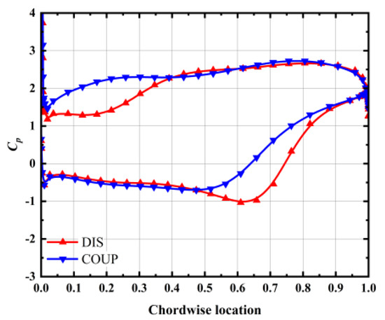
Figure 21.
Comparison of blade loading of different conditions at T/4 (95% spanwise location).
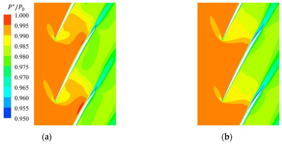
Figure 22.
Comparison of Mach number contours of B2B views at T/4 moment. (a) DIS case; (b) COUP case.
For the inlet distortion condition, the dual shock wave structure in the tip region remains unchanged. However, under the coupling condition, the shock wave angle of the detached bow shock wave increases and the structure of the original shock wave system changes. From Figure 22, the variation in the structure of the coupling condition shock wave system is mainly manifested in two aspects; on the one hand, the shock wave angle of the blade leading edge oblique shock wave increases, and on the other hand, the intensity of the passage normal shock wave is weakened. Under the coupling condition, the shock wave angle of the oblique shock wave at the leading-edge increases, which leads to the intersection point of the shock wave and the adjacent blade suction side to shift forward, and the position of the increased at the suction surface to move forward. At the PE point, the initial location of the passage normal shock wave coincides with the intersection of the oblique shock wave with the suction side of the adjacent blade. Consequently, the intersection point between the channel shock wave and the adjacent blade pressure surface is shifted forward, resulting in the rise point being shifted forward as well.
To manifest the starting position of the shock wave, the slope of and the chordwise location is calculated and the zero slope point is selected. Figure 23 provides the circumferential distribution of the shock wave initial chordwise location under different conditions. At different moments within one revolution, the variation in the shock wave structure under the coupling condition leads to a shift in the shock wave location upstream. The forward shift amount of the shock wave onset position under coupling conditions at different circumferential positions is almost the same, with the shock wave moving upstream by an average of 0.18 chord lengths.
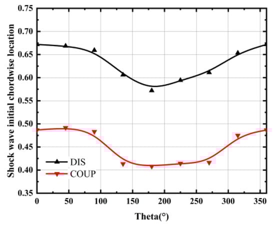
Figure 23.
Comparison of the forward shift in the shock wave initial position of the blade suction surface.
4.4. TLF Structure and Compressor Stability Boundary
Based on the above analyses, the increase in the boundary layer thickness under the coupling condition changes the blade geometry felt by the incoming airflow and affects the structure of the shock wave system in the blade passage, which changes the pressure distribution on the rotor blade surface. At the T/4 moment, the rotor blade is in the transition from the clean to the distortion region, which is the critical region for inducing instability phenomena. The surface pressure distribution on the suction side of the rotor blade under different inflow conditions is shown in Figure 24. Under distortion conditions, the intensity of the shock wave is large, and the flow of the blade suction surface is affected by the shock wave. There is a local high-pressure area after the shock wave in the tip region, and it increases the blade surface radial adverse pressure gradient. Therefore, fluid from the rotor blade hub region migrates radially and streamwise, exiting the blade channel in the mid-spanwise region (shown in Figure 24a). Under coupling conditions, the intensity of the shock wave decreases due to the increase in the thickness of the boundary layer, which weakens the high-pressure area at the trailing edge of the blade to some extent. The adverse pressure gradient along the blade surface in the radial direction is weakened, and the change in the pressure distribution on the suction surface of the rotor blades reduces the pressure gradient in the radial direction, allowing the fluid transported from the blade hub to the tip region (shown in Figure 24b).
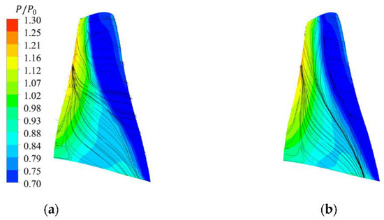
Figure 24.
Comparison of the pressure distribution on the suction surface of the rotor blade. (a) DIS case; (b) COUP case.
Figure 25 shows the radial velocity distribution under distortion and coupling conditions. Compared to the distorted inflow, the radial velocity of the blade rear section increases significantly under the coupling condition. At the trailing edge of the blade, the radial velocity of the blade surface flow increases from 65 m/s (Figure 24a) to 93 m/s (Figure 24a).
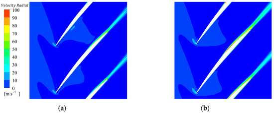
Figure 25.
Comparison of the radial velocity of B2B views at 60% spanwise location. (a) DIS case; (b) COUP case.
Under the coupling condition, the fluid flowing along the radial direction to the tip region affects the structure of the TLF and changes the relative relationship between the tip flows. Figure 26 compares the TLF structure of the rotor blades in the transition zone from the distortion sector to the clean sector. In Figure 26, the solid blue and white lines indicate the streamlines of TLF, and the solid black lines represent the streamlines of fluid flow from the rotor blade hub to the tip region. Under distortion conditions, most of the fluid starting at the rotor blade hub does not reach the tip region and interacts with the TLF (shown in Figure 26a). However, under coupling conditions, the low-energy fluid from the rotor blade hub region flows into the tip region and occupies part of the original TLF area, affecting the relationship between the TLF and the main flow at the tip region. For quantitative assessment, a parameter is introduced to define the relationship between the TLF and the main flow in the tip region. is defined in the following equation:
where represents the axial momentum of the TLF, represents the axial momentum component of the main flow in the tip region. After calculations, for the distortion condition and for the coupling condition. It shows that although the axial velocity of the main flow under the coupling condition is slightly smaller than that under the distortion condition, which reduces the axial momentum of the main flow with the coupling inflow, the axial momentum of the TLF is reduced more significantly due to the variation in the TLF structure, which eventually leads to the reduction in . For the fan stage 67, the decrease in means that the main flow has a stronger dominance against the TLF, which makes it more difficult for the TLF to spill over to the leading edge, at which point the flow state is more stable and unfavorable to the onset of stall.
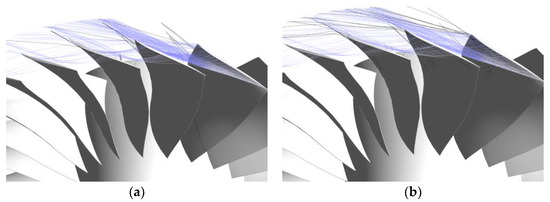
Figure 26.
Comparison of TIF structures under different operating conditions. (a) DIS case; (b) COUP case.
5. Conclusions
In this paper, full-annulus 3D unsteady numerical simulations are conducted for NASA stage 67 under inlet distortion and coupling conditions. The distributions of dimensionless flow parameters, performance loss sources, and TLF structures analyses are carried out, and the fan stage performance and stability boundary changes within coupling inflow are discussed in detail. As the study is conducted for a specific case, the conclusions may not be universal, but some interesting results are still obtained. The concluding elements can be summarized as follows:
Increased losses upstream of the compressor in the coupling case affect the inlet conditions. Losses inside the compressor due to coupling effects are not a linear stack of single factor losses, and additional losses from coupling effects are mainly concentrated in the hub and tip region. The high viscosity of the fluid due to the low Reynolds number increases profile loss over the full circumference in the hub region. Additionally, the increase in shock loss due to the change in shock wave structure under the coupling condition results in additional losses in the tip region.
Compared to the distorted inflow condition, the coupling condition makes the equivalent blade profile thicker. It leads to a variation in the shock wave structure in the rotor blade passage, the shock wave angle of the leading-edge oblique shock wave increases, and the position of the shock wave shifts upstream and finally changes the pressure distribution on the blade surface. The variations in the pressure distribution on the blade surface change the flow structure, and the fluid flowing to the tip region along the radial direction on the blade surface under the coupling condition changes the structure of TLF. The difference in the relationship between the axial momentum components of the main flow and TLF delays the spill over of TLF to the leading edge, which delays the onset of instability.
Author Contributions
Conceptualization, Z.L., T.P. and X.Z.; methodology, X.Z.; software, X.Z. and Z.Y.; validation, X.Z.; formal analysis, X.Z.; investigation, X.Z.; resources, X.Z.; data curation, X.Z.; writing—original draft preparation, X.Z. and Z.Y.; writing—review and editing, T.P. and Z.L.; visualization, X.Z. and Z.Y.; supervision, Z.L. and T.P.; project administration, Z.L. and T.P.; funding acquisition, Z.L. and T.P. All authors have read and agreed to the published version of the manuscript.
Funding
The authors acknowledge the support of the National Natural Science Foundation of China (Nos. 52176032 and 51976005), Advanced Jet Propulsion Creativity Center (Project ID. HKCX2020-02-013), and National Science and Technology Major Project (2017-II-0004-0016 and 2017-II-0005-0018).
Institutional Review Board Statement
Not applicable.
Informed Consent Statement
Not applicable.
Data Availability Statement
Not applicable.
Conflicts of Interest
The authors declare no conflict of interest.
Nomenclature
| additional loss | |
| chord length | |
| DI | distortion intensity |
| boundary layer form factor | |
| m | mass flow |
| momentum | |
| MAPE | mean absolute percentage error |
| total pressure | |
| static pressure | |
| axial momentum ratio of the TLF to main stream | |
| Reynolds number index | |
| entropy | |
| TLF | tip leakage flow |
| static temperature | |
| total temperature | |
| dynamic viscosity coefficient | |
| entropy loss coefficient | |
| total pressure loss coefficient | |
| profile loss | |
| shock loss | |
| boundary layer momentum thickness | |
| air angle measured from axial direction | |
| blade angle of attack | |
| Subscripts: | |
| a | axial direction |
| cor | corrected |
| clean | clean sector |
| COUP | coupling condition |
| dis | distortion sector |
| DIS | distortion condition |
| sea | sea level |
| Min | minimum |
References
- Ehrich, F. Circumferential Inlet Distortions in Axial Flow Turbomachinery. J. Aeronaut. Sci. 1957, 24, 413–417. [Google Scholar] [CrossRef]
- Seidel, B.S. Asymmetric Inlet Flow in Axial Turbomachines. J. Eng. Power 1964, 86, 18–28. [Google Scholar] [CrossRef]
- Greitzer, E.M. Upstream Attenuation and Quasi-Steady Rotor Lift Fluctuations in Asymmetric Flows in Axial Flow Compressors. In Proceedings of the ASME 1973 International Gas Turbine Conference and Products Show, Washington, DC, USA, 8–12 April 1973. [Google Scholar] [CrossRef]
- Biesiadny, T.J.; Braithwaite, W.M.; Soeder, R.H.; Abdelwahab, M. Summary of Investigations of Engine Response to Distorted Inlet Conditions. Available online: https://ntrs.nasa.gov/citations/19860016864 (accessed on 20 April 2022).
- Reid, C. The Response of Axial Flow Compressors to Intake Flow Distortion. In Proceedings of the ASME 1969 Gas Turbine Conference and Products Show, Cleveland, OH, USA, 9–13 March 1969. [Google Scholar]
- Longley, J.P. Measured and Predicted Effects of Inlet Distortion on Axial Compressors. In Proceedings of the ASME 1990 International Gas Turbine and Aeroengine Congress and Exposition, Brussels, Belgium, 11–14 June 1990. [Google Scholar]
- Longley, J.P.; Shin, H.W.; Plumley, R.E.; Silkowski, P.D.; Day, I.J.; Greitzer, E.M.; Tan, C.S.; Wisler, D.C. Effects of Rotating Inlet Distortion on Multistage Compressor Stability. J. Turbomach. 1996, 118, 181–188. [Google Scholar] [CrossRef]
- Gunn, E.J.; Tooze, S.E.; Hall, C.A.; Colin, Y. An Experimental Study of Loss Sources in a Fan Operating with Continuous Inlet Stagnation Pressure Distortion. J. Turbomach. 2013, 135, 051002. [Google Scholar] [CrossRef]
- Rademakers, R.P.M.; Bindl, S.; Niehuis, R. Effects of Flow Distortions as They Occur in S-Duct Inlets on the Performance and Stability of a Jet Engine. J. Eng. Gas Turbines Power 2016, 138, 022605. [Google Scholar] [CrossRef]
- Naseri, A.; Sammak, S.; Boroomand, M.; Alihosseini, A.; Tousi, A.M. Experimental Investigation of Inlet Distortion Effect on Performance of a Micro Gas Turbine. J. Eng. Gas Turbines Power 2018, 140, 092604. [Google Scholar] [CrossRef]
- Perovic, D.; Hall, C.A.; Gunn, E.J. Stall Inception in a Boundary Layer Ingesting Fan. J. Turbomach. 2019, 141, 091007. [Google Scholar] [CrossRef]
- Fidalgo, V.J.; Hall, C.A.; Colin, Y. A Study of Fan-Distortion Interaction within the NASA Rotor 67 Transonic Stage. J. Turbomach. 2012, 134, 051011. [Google Scholar] [CrossRef]
- Zhang, W.; Vahdati, M. Influence of the Inlet Distortion on Fan Stall Margin at Different Rotational Speeds. In Proceedings of the GPPS Conference, Shanghai, China, 30 October–1 November 2017. [Google Scholar]
- Zhang, W.; Stapelfeldt, S.; Vahdati, M. Influence of the Inlet Distortion on Fan Stall Margin at Different Rotational Speeds. Aerosp. Sci. Technol. 2020, 98, 105668. [Google Scholar] [CrossRef]
- Zhang, W.; Vahdati, M. A Parametric Study of the Effects of Inlet Distortion on Fan Aerodynamic Stability. J. Turbomach. 2019, 141, 011011. [Google Scholar] [CrossRef]
- Zhang, W.; Vahdati, M. Stall and Recovery Process of a Transonic Fan With and Without Inlet Distortion. J. Turbomach. 2019, 142, 011003. [Google Scholar] [CrossRef]
- Ma, Y.; Cui, J.; Vadlamani, N.R.; Tucker, P. A Mixed-Fidelity Numerical Study for Fan–Distortion Interaction. J. Turbomach. 2018, 140, 091003. [Google Scholar] [CrossRef]
- Wallner, L.E.; Lubick, R.J.; Chelko, L.J. Preliminary Results of the Determination of Inlet-Pressure Distortion Effects on Compressor Stall and Altitude Operating Limits of the J57-P-1 Turbojet Engine. Available online: https://ntrs.nasa.gov/citations/20090023603 (accessed on 20 April 2022).
- Cousins, W.T.; Dalton, K.K.; Andersen, T.T.; Bobula, G.A. Pressure and Temperature Distortion Testing of a Two-Stage Centrifugal Compressor. In Proceedings of the International Gas Turbine and Aeroengine Congress and Exposition, Cincinnati, OH, USA, 24–27 May 1993. [Google Scholar]
- Lee, K.; Lee, B.; Kang, S.; Yang, S.; Lee, D. Inlet Distortion Test with Gas Turbine Engine in the Altitude Engine Test Facility. In Proceedings of the 27th AIAA Aerodynamic Measurement Technology and Ground Testing Conference, Chicago, IL, USA, 28 June–1 July 2010. [Google Scholar] [CrossRef]
- Strazisar, A.J.; Wood, J.R.; Hathaway, M.D.; Suder, K.L. Laser Anemometer Measurements in a Transonic Axial-Flow Fan Rotor. J. Eng. Gas Turbines Power 1981, 103, 430–437. [Google Scholar] [CrossRef]
- Van Zante, D.E.; Podboy, G.G.; Miller, C.J.; Thorp, S.A. Testing and Performance Verification of a High Bypass Ratio Turbofan Rotor in an Internal Flow Component Test Facility. In Proceedings of the 27th AIAA Aerodynamic Measurement Technology and Ground Testing Conference, Chicago, IL, USA, 28 June–1 July 2010. [Google Scholar]
- Spotts, N. Unsteady Reynolds-Averaged Navier-Stokes Simulations of Inlet Flow Distortion in the Fan System of a Gas-Turbine Aero-Engine; Colorado State University: Fort Collins, CO, USA, 2015. [Google Scholar]
- Lake, J.; King, P.; Rivir, R. Reduction of Separation Losses on a Turbine Blade with Low Reynolds Numbers. In Proceedings of the 37th Aerospace Sciences Meeting and Exhibit, Reno, NV, USA, 11–14 January 1999. [Google Scholar] [CrossRef]
- Bons, J.; Sondergaard, R.; Rivir, R. Control of Low-Pressure Turbine Separation Using Vortex Generator Jets. In Proceedings of the 37th Aerospace Sciences Meeting and Exhibit, Reno, NV, USA, 11–14 January 1999. [Google Scholar]
- Huang, J.; Corke, T.C.; Thomas, F.O. Plasma Actuators for Separation Control of Low-Pressure Turbine Blades. AIAA J. 2006, 44, 51–57. [Google Scholar] [CrossRef]
- Yang, Z.; Lu, H.; Pan, T.; Li, Q. Numerical Investigation on the Influences of Boundary Layer Ingestion on Tip Leakage Flow Structures and Losses in a Transonic Axial-Flow Fan. J. Fluids Eng. 2021, 143, 111207. [Google Scholar] [CrossRef]
- Boyer, K.M.; O’Brien, W.F. An Improved Streamline Curvature Approach for Off-Design Analysis of Transonic Axial Compression Systems. J. Turbomach. 2003, 125, 475–481. [Google Scholar] [CrossRef]
- König, W.M.; Hennecke, D.K.; Fottner, L. Improved Blade Profile Loss and Deviation Angle Models for Advanced Transonic Compressor Bladings: Part I—A Model for Subsonic Flow. J. Turbomach 1996, 118, 73–80. [Google Scholar] [CrossRef]
- König, W.M.; Hennecke, D.K.; Fottner, L. Improved Blade Profile Loss and Deviation Angle Models for Advanced Transonic Compressor Bladings: Part II—A Model for Supersonic Flow. J. Turbomach 1996, 118, 81–87. [Google Scholar] [CrossRef]
- Koch, C.C.; Smith, L.H., Jr. Loss Sources and Magnitudes in Axial-Flow Compressors. J. Eng. Power 1976, 98, 411–424. [Google Scholar] [CrossRef]
- Bloch, G.S.; Copenhaver, W.W.; O’Brien, W.F. A Shock Loss Model for Supersonic Compressor Cascades. J. Turbomach. 1999, 121, 28–35. [Google Scholar] [CrossRef]


Publisher’s Note: MDPI stays neutral with regard to jurisdictional claims in published maps and institutional affiliations. |
© 2022 by the authors. Licensee MDPI, Basel, Switzerland. This article is an open access article distributed under the terms and conditions of the Creative Commons Attribution (CC BY) license (https://creativecommons.org/licenses/by/4.0/).