
ADRC Control System of PMLSM Based on Novel Non-Singular Terminal Sliding Mode Observer


Abstract
:1. Introduction
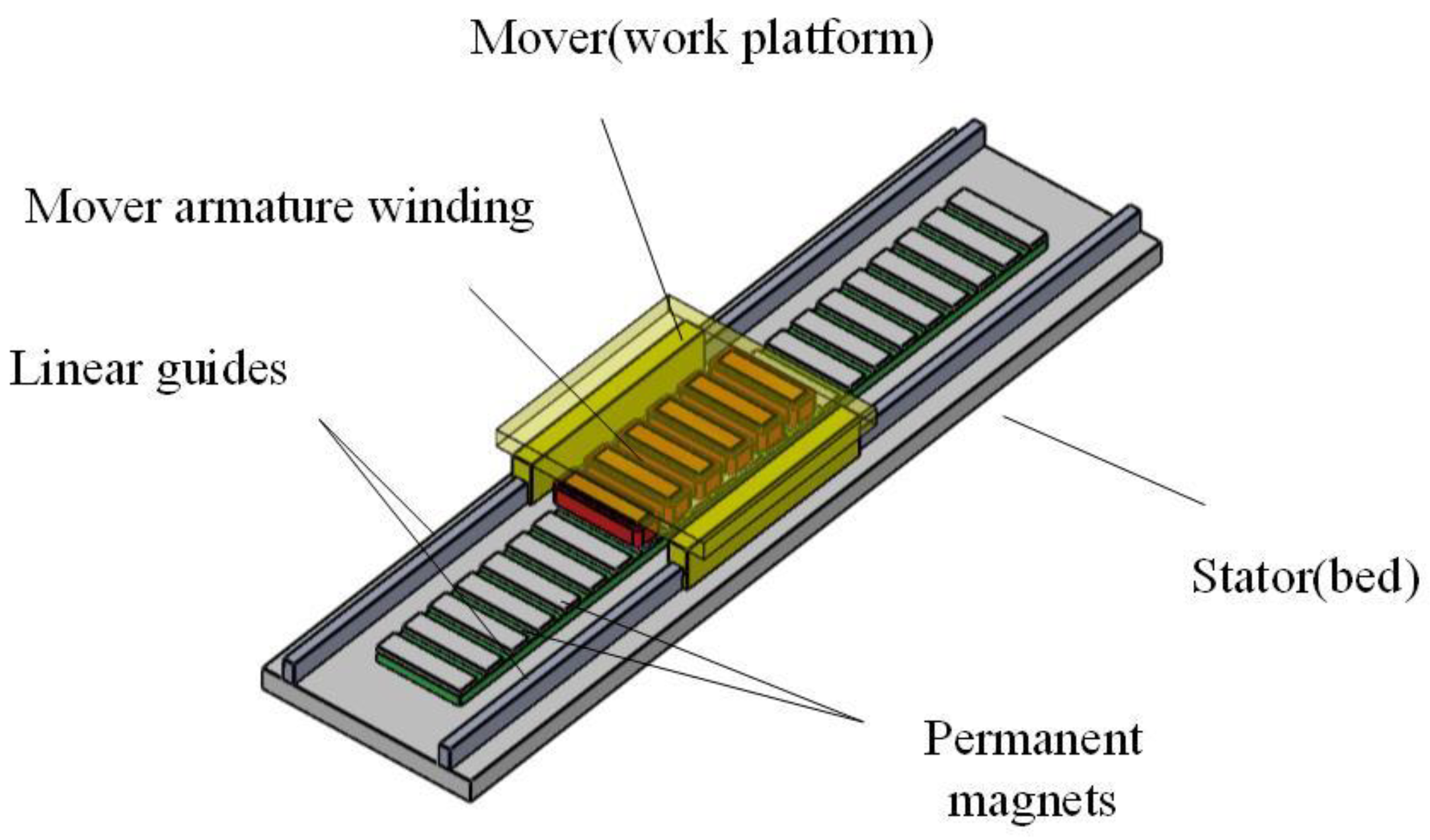
2. Mathematical Model of PMLSM
3. Active Disturbance Rejection Integrated Controller
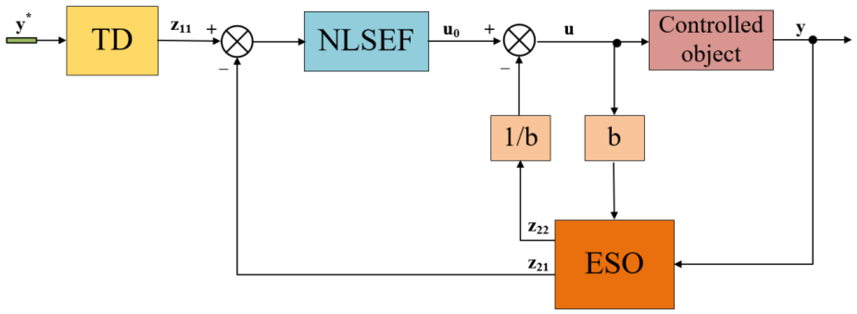
3.1. Traditional ADRC
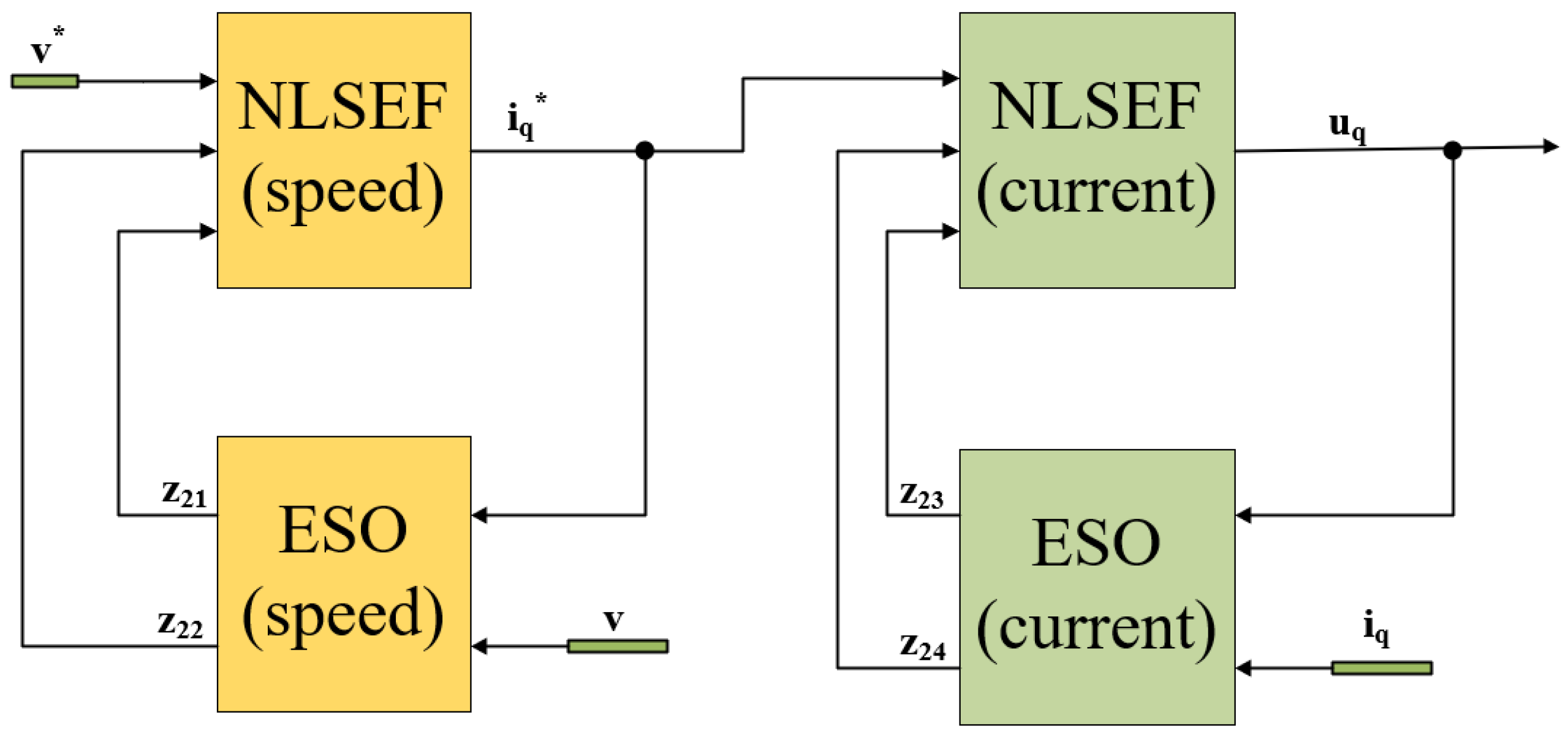
3.2. The Simplified Design of Active Disturbance Rejection Integrated Controller
3.2.1. Design of Active Disturbance Rejection Controller for Velocity Loop
3.2.2. Design of Active Disturbance Rejection Controller for Current Loop
4. Design of a Non-Singular Terminal SMO
4.1. Non-Singular Fast Terminal Sliding Surface
4.2. Design of Non-Singular Terminal SMO
4.3. Stability Analysis
4.4. Track Differentiator Settings
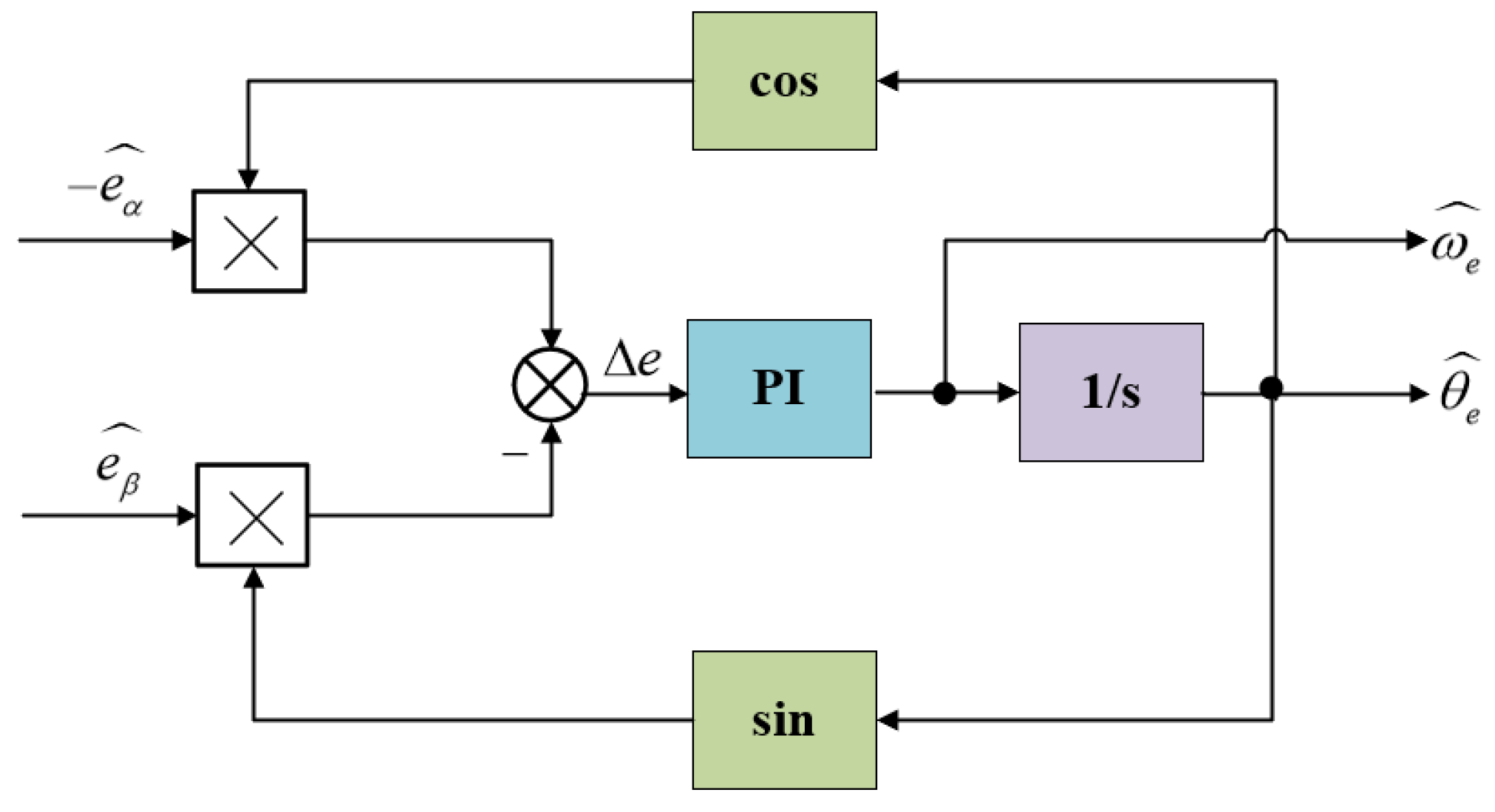
4.5. PLL Policy Application
5. Simulation and Experimental Results
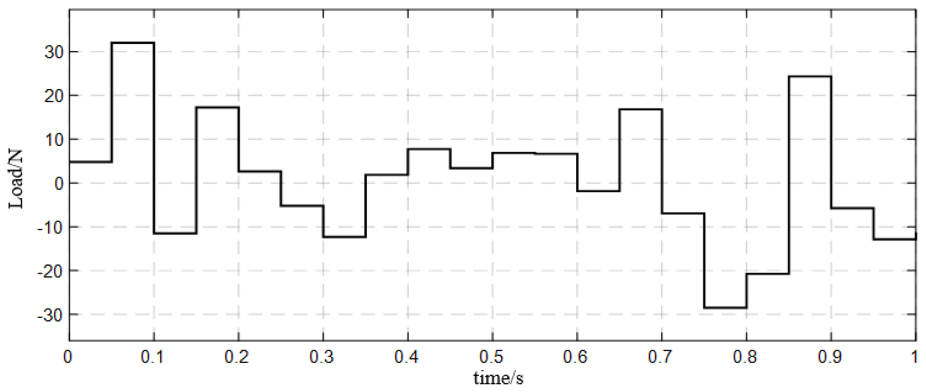
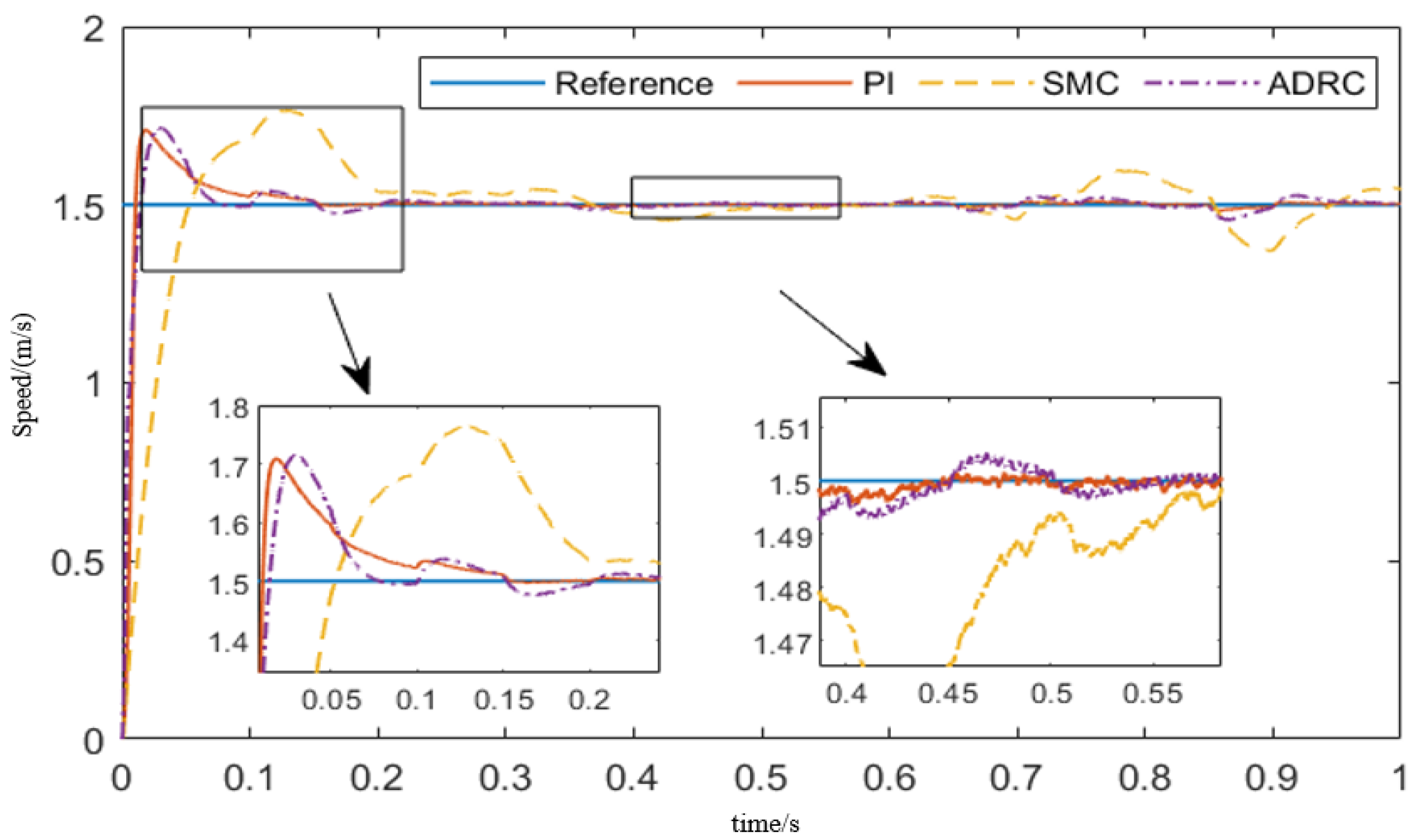
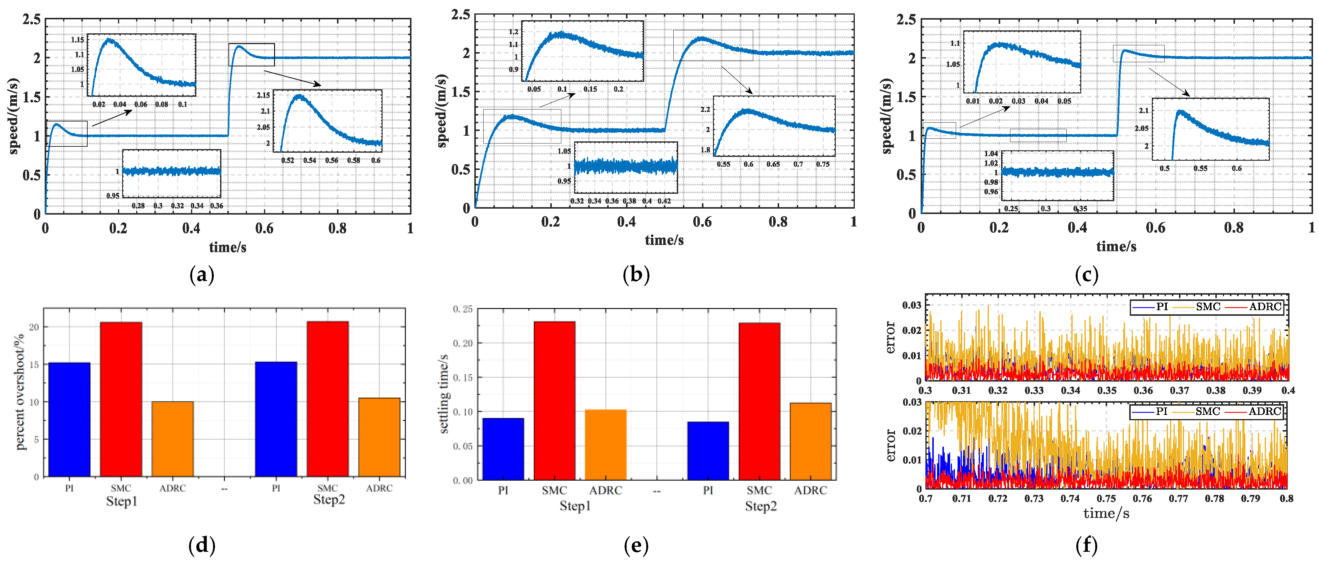
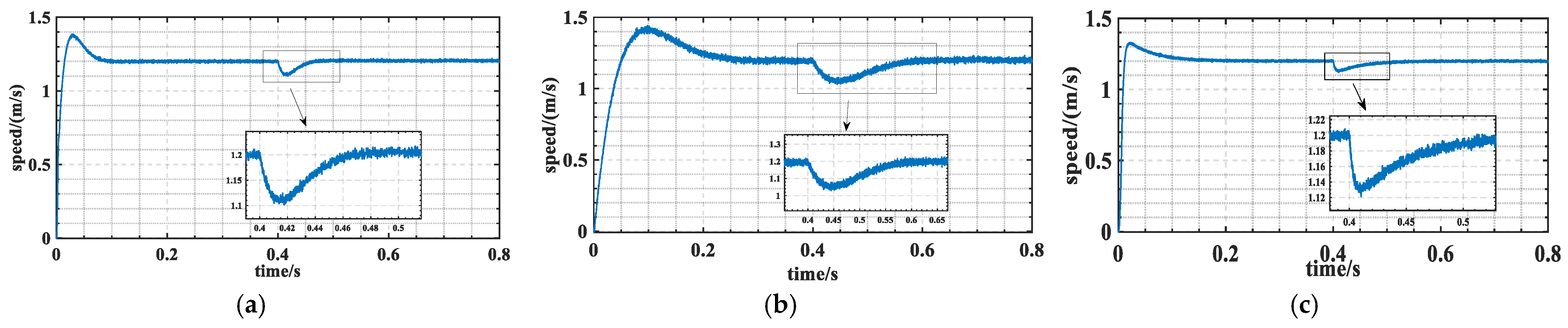
5.1. Simulation
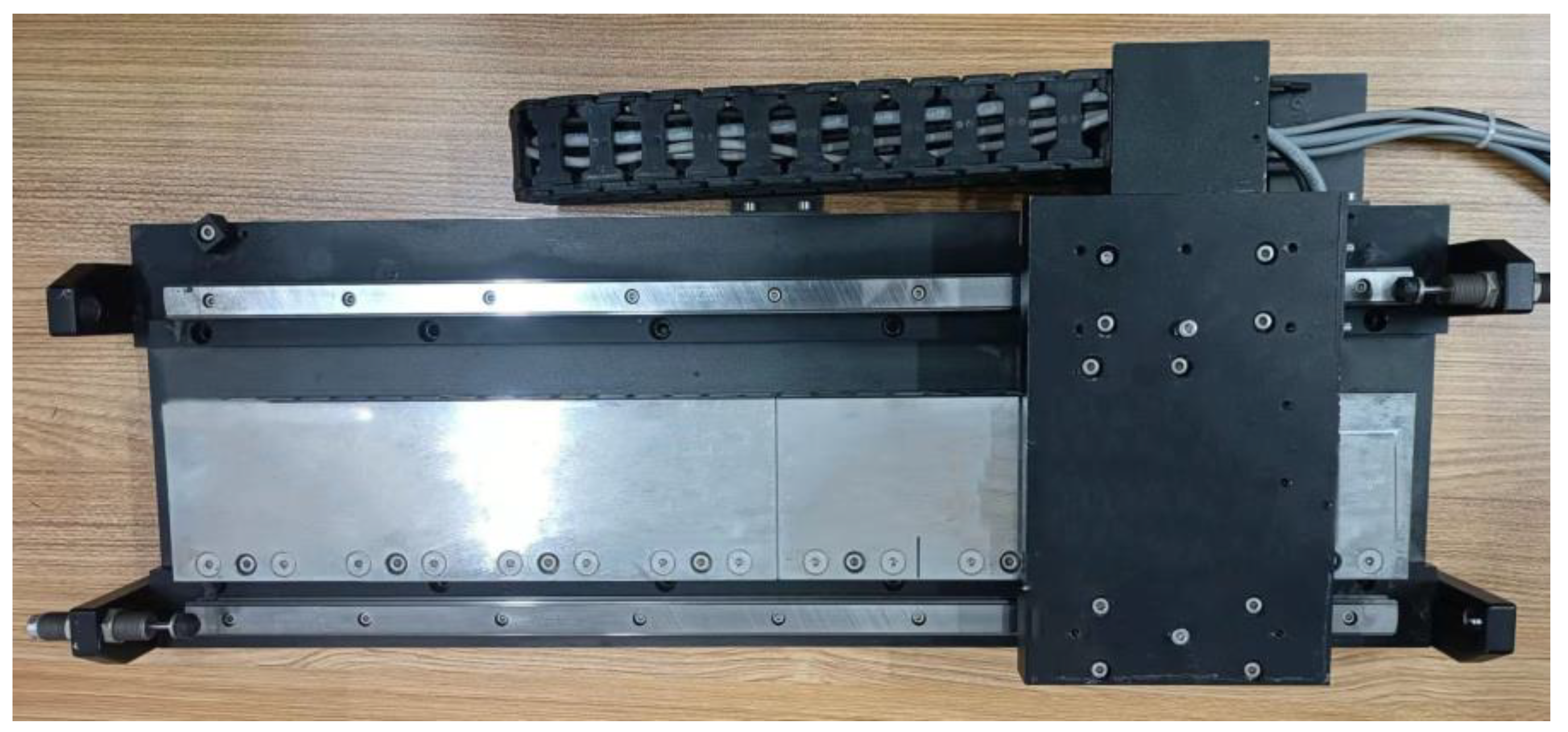
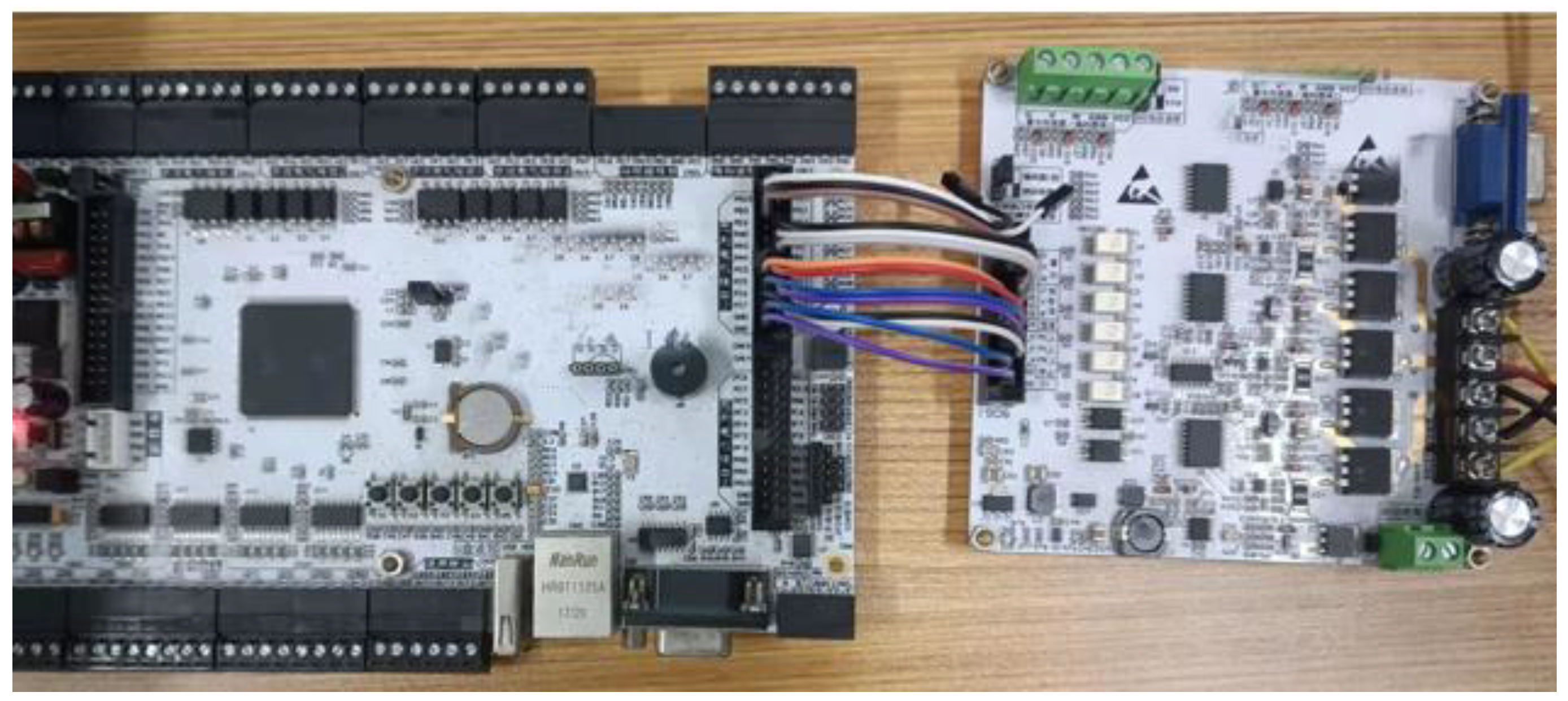
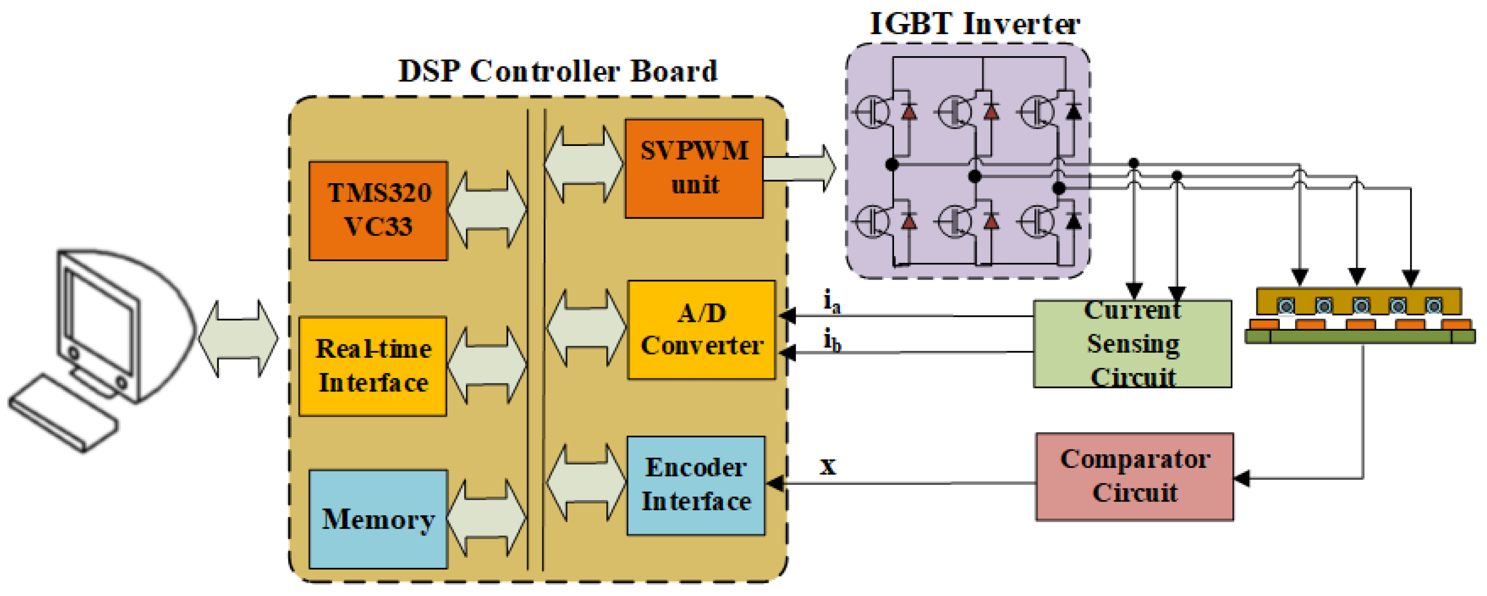
5.2. Experiment
6. Conclusions
Author Contributions
Funding
Conflicts of Interest
References
- Yang, R.; Li, L.; Wang, M.; Zhang, C. Force Ripple Compensation and Robust Predictive Current Control of PMLSM Using Augmented Generalized Proportional–Integral Observer. IEEE J. Emerg. Sel. Top. Power Electron. 2021, 9, 302–315. [Google Scholar] [CrossRef]
- Dong, F.; Zhao, J.; Zhao, J.; Song, J.; Chen, J.; Zheng, Z. Robust Optimization of PMSLM Based on a New Filled Function Algorithm With a Sigma Level Stability Convergence Criterion. IEEE Trans. Ind. Inform. 2021, 17, 4743–4754. [Google Scholar] [CrossRef]
- Yang, R.; Wang, M.; Li, L.; Wang, G.; Zhong, C. Robust Predictive Current Control of PMSLM With Extended State Modeling Based Kalman Filter: For Time-Varying Disturbance Rejection. IEEE Trans. Power Electron. 2020, 35, 2208–2221. [Google Scholar] [CrossRef]
- Cui, F.; Sun, Z.; Xu, W.; Qian, H.; Cao, C. Optimization Analysis of Long Primary Permanent Magnet Linear Synchronous Motor. IEEE Trans. Appl. Supercond. 2021, 31, 1–4. [Google Scholar] [CrossRef]
- Zhao, J.; Mou, Q.; Zhu, C.; Chen, Z.; Li, J. Study on a Double-Sided Permanent-Magnet Linear Synchronous Motor With Reversed Slots. IEEE/ASME Trans. Mechatron. 2021, 26, 3–12. [Google Scholar] [CrossRef]
- Liu, Y.; Gao, J.; Zhong, Y.; Zhang, L. Extended State Observer-Based IMC-PID Tracking Control of PMSLM Servo Systems. IEEE Access 2021, 9, 29036–49046. [Google Scholar]
- Hamed, H.A.; El-Barbary, Z.; Moursi, M.S.; Chamarthi, P.K. A New δ-MRAS Method For Motor Speed Estimation. IEEE Trans. Power Deliv. 2020, 36, 1903–1906. [Google Scholar] [CrossRef]
- Xu, W.; Junejo, A.K.; Tang, Y.; Shahab, M.; Habib, H.U.R.; Liu, Y.; Huang, S. Composite Speed Control of PMSM Drive System Based on Finite Time Sliding Mode Observer. IEEE Access 2021, 9, 151803–151813. [Google Scholar] [CrossRef]
- Hao, Z.; Yang, Y.; Gong, Y.; Hao, Z.; Zhang, C.; Song, H.; Zhang, J. Linear/Nonlinear Active Disturbance Rejection Switching Control for Permanent Magnet Synchronous Motors. IEEE Trans. Power Electron. 2021, 36, 9334–9347. [Google Scholar] [CrossRef]
- Zuo, Y.; Mei, J.; Jiang, C.; Yuan, X.; Xie, S.; Lee, C.H.T. Linear Active Disturbance Rejection Controllers for PMSM Speed Regulation System Considering the Speed Filter. IEEE Trans. Power Electron. 2021, 36, 14579–14592. [Google Scholar] [CrossRef]
- Lin, P.; Wu, Z.; Liu, K.-Z.; Sun, X.-M. A Class of Linear–Nonlinear Switching Active Disturbance Rejection Speed and Current Controllers for PMSM. IEEE Trans. Power Electron. 2021, 36, 14366–14382. [Google Scholar] [CrossRef]
- Chen, S.; Zhao, Y.; Qiu, H.; Ren, X. High-Precision Rotor Position Correction Strategy for High-Speed Permanent Magnet Synchronous Motor Based on Resolver. IEEE Trans. Power Electron. 2020, 35, 9716–9726. [Google Scholar] [CrossRef]
- Colombo, L.; Corradini, M.L.; Cristofaro, A.; Ippoliti, G.; Orlando, G. An Embedded Strategy for Online Identification of PMSM Parameters and Sensorless Control. IEEE Trans. Control Syst. Technol. 2019, 27, 2444–2452. [Google Scholar] [CrossRef]
- de Castro, A.G.; Guazzelli, P.R.U.; de Oliveira, C.M.R.; Pereira, W.C.D.A.; de Paula, G.T.; Monteiro, J.R.B.D.A. Optimized Current Waveform for Torque Ripple Mitigation and MTPA Operation of PMSM with Back EMF Harmonics based on Genetic Algorithm and Artificial Neural Network. IEEE Lat. Am. Trans. 2020, 9, 1646–1655. [Google Scholar] [CrossRef]
- Du, B.; Zhao, T.; Han, S.; Song, L.; Cui, S. Sensorless Control Strategy for IPMSM to Reduce Audible Noise by Variable Frequency Current Injection. IEEE Trans. Ind. Electron. 2020, 67, 1149–1159. [Google Scholar] [CrossRef]
- Cheng, H.; Sun, S.; Zhou, X.; Shao, D.; Mi, S.; Hu, Y. Sensorless DPCC of PMLSM Using SOGI-PLL-Based High-Order SMO With Cogging Force Feedforward Compensation. IEEE Trans. Transp. Electrif. 2022, 8, 1094–1104. [Google Scholar] [CrossRef]
- Li, Z.; Zhou, S.; Xiao, Y.; Wang, L. Sensorless Vector Control of Permanent Magnet Synchronous Linear Motor Based on Self-Adaptive Super-Twisting Sliding Mode Controller. IEEE Access 2019, 7, 44998–45011. [Google Scholar] [CrossRef]
- Xu, B.; Zhang, L.; Ji, W. Improved Non-Singular Fast Terminal Sliding Mode Control With Disturbance Observer for PMSM Drives. IEEE Trans. Transp. Electrif. 2021, 7, 2753–2762. [Google Scholar] [CrossRef]
- Fu, D.; Zhao, X.; Zhu, J. A Novel Robust Super-Twisting Nonsingular Terminal Sliding Mode Controller for Permanent Magnet Linear Synchronous Motors. IEEE Trans. Power Electron. 2022, 37, 2936–2945. [Google Scholar] [CrossRef]
- Shao, K.; Zheng, J.; Huang, K.; Wang, H.; Man, Z.; Fu, M. Finite-Time Control of a Linear Motor Positioner Using Adaptive Recursive Terminal Sliding Mode. IEEE Trans. Ind. Electron. 2020, 67, 6659–6668. [Google Scholar] [CrossRef]


| Parameter | Value |
|---|---|
| stator resistance Rs/Ω | 4.0 |
| d-q axis inductance Ldq/mH | 8.2 |
| Mover mass m/kg | 1.425 |
| Viscous friction coefficient B/N/m⋅s | 44 |
| Polar distance τ/m | 0.016 |
| DC Bus Voltage U/V | 200 |
Publisher’s Note: MDPI stays neutral with regard to jurisdictional claims in published maps and institutional affiliations. |
© 2022 by the authors. Licensee MDPI, Basel, Switzerland. This article is an open access article distributed under the terms and conditions of the Creative Commons Attribution (CC BY) license (https://creativecommons.org/licenses/by/4.0/).
Share and Cite
Li, Z.; Zhang, Z.; Wang, J.; Wang, S.; Chen, X.; Sun, H. ADRC Control System of PMLSM Based on Novel Non-Singular Terminal Sliding Mode Observer. Energies 2022, 15, 3720. https://doi.org/10.3390/en15103720
Li Z, Zhang Z, Wang J, Wang S, Chen X, Sun H. ADRC Control System of PMLSM Based on Novel Non-Singular Terminal Sliding Mode Observer. Energies. 2022; 15(10):3720. https://doi.org/10.3390/en15103720
Chicago/Turabian StyleLi, Zheng, Zihao Zhang, Jinsong Wang, Shaohua Wang, Xuetong Chen, and Hexu Sun. 2022. "ADRC Control System of PMLSM Based on Novel Non-Singular Terminal Sliding Mode Observer" Energies 15, no. 10: 3720. https://doi.org/10.3390/en15103720