Abstract
From a practical point of view, a turbine load cycle (TLC) is defined as the time a turbine in a power plant remains in operation. TLC is used by many electric power plants as a stop indicator for turbine maintenance. In traditional operations, a maximum time for the operation of a turbine is usually estimated and, based on the TLC, the remaining operating time until the equipment is subjected to new maintenance is determined. Today, however, a better process is possible, as there are many turbines with sensors that carry out the telemetry of the operation, and machine learning (ML) models can use this data to support decision making, predicting the optimal time for equipment to stop, from the actual need for maintenance. This is predictive maintenance, and it is widely used in Industry 4.0 contexts. However, knowing which data must be collected by the sensors (the variables), and their impact on the training of an ML algorithm, is a challenge to be explored on a case-by-case basis. In this work, we propose a framework for mapping sensors related to a turbine in a hydroelectric power plant and the selection of variables involved in the load cycle to: (i) investigate whether the data allow identification of the future moment of maintenance, which is done by exploring and comparing four ML algorithms; (ii) discover which are the most important variables (MIV) for each algorithm in predicting the need for maintenance in a given time horizon; (iii) combine the MIV of each algorithm through weighting criteria, identifying the most relevant variables of the studied data set; (iv) develop a methodology to label the data in such a way that the problem of forecasting a future need for maintenance becomes a problem of binary classification (need for maintenance: yes or no) in a time horizon. The resulting framework was applied to a real problem, and the results obtained pointed to rates of maintenance identification with very high accuracies, in the order of 98%.
1. Introduction
The use of new technologies, such as the Internet of Things (IoT), artificial intelligence (AI) and big data processes, has been leveraged by the possibility of collecting and processing large volumes of data [1]. This phenomenon in the industrial segment has enabled the implementation of data-driven decisions, with the new vision of Industry 4.0. An example of this is the improvement in the performance of operations in industries due to the continuous monitoring of equipment, feeding the decision-making process and predictive maintenance [2,3,4].
Data-driven decisions in the case of predictive maintenance management (PdM) are made by monitoring industrial equipment variables and their association with the statistical behavior of historical data. This constitutes the basis for the construction of mathematical models, based on machine learning (ML) algorithms, which, according to [5], are nothing more than a subarea of AI. These ML models are implemented in computational tools, aimed at supporting PdM decisions.
With the use of these ML models, the scheduling of equipment downtime for maintenance is based on forecasts generated by the models and not on times with fixed intervals between stops, which would actually be a preventive and not a predictive maintenance. The “optimal” downtime for maintenance, therefore, is now established based on a prediction of an ML model, which has been previously calibrated (trained) based on historical operating data. It is this forecasting approach, supported by models, that characterizes the so-called predictive maintenance [6,7].
Due to the complexity of the number of variables that may be available for a PdMspecific set of data associated with the workload cycle (LC) of the equipment, and regarding the use of LC, it should be considered that in the process of developing predictive models, one of the key issues is the definition of the data attributes (relevant variables) that will be used in the models. In the case of PdM, there can be several factors that can lead to an outage due to the failure of some component. This research adopted as a basic hypothesis the consideration that the most relevant factor positively impacting the probability of a failure in industrial equipment is its LC. Thus, using a direct measure of LC and other indirect metrics, derived from LC, in the composition of a predictive model, it was possible to have an effective strategy to predict the occurrence of a failure in the equipment.
In a previous work [8] has already explored the use of ML models in PdM, which includes a proposal for a methodological framework covering all the stages of a Big Data process, from the mapping of the system, the pre-processing of variables and an implementation of decision tree modeling for PdM.
In this paper, the framework was expanded to use a set of historical data with values collected from the variables associated with the LC, with the respective timestamps of each data point collected. From this database, it is possible to identify for each instance (each example) of the occurrence or not of a failure in fixed future periods of 12 h, 24 h and 48 h, from the instant associated with that instance. With this, it is possible to build a predictive model which, considering only the current conditions of these variables, would be able to project the occurrence of a failure in the considered time horizons.
The article presents a real-world case uncommon in the literature, which is the application of PdM in a hydroelectric power plant. The real case in the article deals with the LC of a turbine of a power generation unit of the plant, composed of a turbine and generator.
The whole set of theoretical and practical contributions of the paper are presented in Section 1.4.
In terms of results, the proposed framework proved to be adequate for this type of study and the predictive models, based on LC, reached accuracy levels in the order of 98%.
1.1. Motivation
The challenge of developing a predictive modeling process based on ML, as the one proposed here, is already a considerable challenge that is highly motivating for researchers in this field. Furthermore, the process and models proposed here can be considered a framework to be adapted to any future projects of predictive maintenance. In addition, the study was carried out in the real industrial environment of an old Brazilian company, which has been trying over the years to adapt its processes and systems to the new concepts of Industry 4.0, and this project is part of this challenge.
Therefore, there are a set of motivations for carrying out this study, and to be able to report in the literature the experience obtained in this research applied in a real-world case, may bring some contribution to the advancement of knowledge in this area.
1.2. Research Question
This subsection presents the research question (RQ), subdivided in two parts, that drove the development of the study described in the paper.
- RQ:
- Is it feasible to develop a consistent predictive model based on variables associated with the LC of industrial equipment to forecast this equipment failure on a future period?
- What would be the phases, techniques, algorithms and variables to be considered in the model, in order to constitute a consistent framework, focused on this modeling process, considering that it must be applied in real cases of PdM in an industrial environment?
As the question puts, its objective is to define the phases, techniques and algorithms that should be used in the modeling process, based on variables related to the LC of equipment, thus defining a framework to solve this type of problem. Such a framework must be suitable for application in real cases of predictive maintenance.
1.3. Objectives
Based on the RQ, the objective of this study, therefore, is to address the development and application of a predictive maintenance modeling process, which can be constituted in a framework to be applied in other instances and should be developed through a modeling process based on the LC of the equipment.
As specific objectives of the study, the following aspects should be addressed:
- (a)
- Define the phases to achieve an effective modeling process, from collecting data to implementing a model and obtaining its results;
- (b)
- Define these phases and the model configuration so that they can be a framework to be applied in different instances and based on different techniques;
- (c)
- Define the variables to be considered in the model based on the accuracy criteria of model outputs;
- (d)
- Define machine learning algorithms to be applied in the model construction, based on the accuracy criteria of model outputs;
- (e)
- Develop strategies and techniques to train, validate and reduce model dimensionality;
- (f)
- Apply the resulting structure in a real-world case in an hydroelectric power plant environment.
1.4. Implications and Contributions
This work may imply theoretical contributions to PdM and practical contributions to operations in power plants, particularly for hydroelectric power plants, which are rarely mentioned in the literature, with regard to PdM. In general, the contribution of work can be defined as follows:
Theoretical Contributions:
- Use of a direct measure of the Load Cycle—LC, of the equipment and other indirect metrics, derived from LC, in the composition of a predictive model;
- Development of data modeling and creation of new labels, which allowed treatment of the problem of predicting an occurrence at a future time as a data classification task;
- Development of a detailed methodological framework covering all the stages of Big Data processes;
- Include in the framework a mapping of the system for the identification of the relevant variables for modeling;
- Development of a composite global score for the most important variables—MIV, considering the level of importance of the variable in each model explored.
Practical Contributions:
- Development of an application in hydroelectric turbines. We did not find in the literature any study of this type in hydroelectric power plants;
- Implementation of a detailed methodological framework covering all the stages of Big Data processes;
- Development of a mapping of the system and identification of the relevant variables for the PdM modeling;
- Development of a broad analysis of the importance of variables of the predictive models, discussing concepts and computational processes for measuring the level of importance of variables in each type of predictive model;
- Analysis of the performance of predictive models exploring various indicators, which is not common in the literature;
- Development of data modeling and creation of new labels, which allowed the prediction of equipment failures in different time horizons, specifically for 12 h, 24 h and 48 h horizons.
These points represent contributions that may serve as a reference for future work.
In addition to this Introduction, this article has four more sections. The next section, Section 2, discusses a series of papers related to the study developed here. Section 3 describes the proposed methodological framework, covering all the stages of a big data process. Section 4 presents a case study, which represents an extensive real-world application, where all stages of the process are discussed. Finally, Section 5 presents the conclusions of the study and recommendations for future work.
2. Related Work
The industry is experiencing the so-called Fourth Industrial Revolution or Industry 4.0. This concept concerns the use of technologies that allow the integration of equipment (physical systems) with software (digital systems) in industrial environments. This makes it possible to collect a large amount of data (Big Data) through sensors (Internet of Things IoT), enabling the use of this data for decision making, since there is a faster and more targeted exchange of information [1].
According to [3], the concept of Industry 4.0 emerged in Germany, in 2011, in a research group made up of representatives of the German government and companies, seeking a common framework for the application of such technologies as IoT, wireless sensors (WS) and sensor networks (WSN), cloud computing and cyber physical systems (CPS). Different terms were used to designate Industry 4.0, such as: Smart Manufacturing, Smart Production, Industrial Internet, i4.0, Connected Industry 4.0.
One of the important points of Industry 4.0 is the use of AI/ML in predictive maintenance processes, which is one of the maintenance strategies.
The papers [6,7] classify maintenance strategies into the following categories:
- Run-to-failure (R2F) or corrective maintenance;
- Preventive maintenance (PvM) or scheduled maintenance;
- Condition-based maintenance (CBM) and
- Predictive maintenance (PdM) or statistical-based maintenance.
In R2F, maintenance occurs after an equipment failure. It is the simplest strategy, but the most expensive, as there is an unexpected interruption in the operation of equipment and/or processes, in addition, repairs can be greater and longer than they could have been if the stoppage had occurred earlier.
In the case of PvM, maintenance is carried out according to a maintenance plan in which each piece of equipment follows a stop schedule, according to its characteristics and LC. This procedure usually anticipates failures, but, on the other hand, unnecessary stoppage is sometimes performed, when the equipment deterioration prediction does not materialize.
In the CBM procedure, there is a continuous monitoring of the health of the equipment or process. This allows you to identify when maintenance is really needed. On the other hand, it is not possible to plan maintenance in advance.
PdM is a strategy that develops an equipment or process failure prediction, based on a prediction model. These models can represent the physical behavior of the equipment or they can be based on data collected about the equipment/process, using, in this case, statistical inference or artificial intelligence (machine learning) models.
Other authors attribute different meanings to these terms. In [9], for example, they invert the concepts of CBM and PdM. In fact, they consider that it is in the PdM strategy that the health status of the equipment is continuously monitored and that this verification is even done manually.
On the other hand, in a recent paper [10] the authors state that PdM can still be called on-line monitoring or risk-based maintenance, and that PdM and CBM are the same. They say that PdM has evolved from visual inspection to automated methods, utilizing pattern recognition, machine learning, neural networks, fuzzy logic, etc.
In another paper [11], the authors say that CBM is often used as a synonym for PdM, and [12] view CBM as a subcategory of PdM, subdividing PdM into two types: statistical PdM and condition-based PdM, where statistical PdM focuses on classification, while most studies of condition-based PdM have focused on regression.
As can be seen, there is no absolute agreement among the authors, regarding the terms that designate the different maintenance strategies, but for the purpose of this work, the definitions given by [6,7] will be adopted.
Now, regarding the techniques applied to PdM, there are a variety of ML algorithms that have been used to support maintenance management. There are ML algorithms of various types in use, such as tree-based algorithms, instance based learning (IBL), probabilistic, network-based algorithms, regression, metaheuristics, etc.
Some examples of tree-based techniques are decision tree (DT) [8,13,14], as well as random forest (RF) [14,15]. Applications of a traditional IBL algorithm, the K-nearest neighbor (K-NN), are presented in [7,14]. About probabilistic algorithms, applications of the classic Naïve Bayes (NB) and a Bayesian network (BN) can be found in [14]. Different cases of artificial neural networks (ANN) are presented in [13,14,15,16,17,18]. Applications of support vector machines (SVM) are discussed in [7,14,19,20,21]. Regarding regression, applications based on logistic regression (LR) can be seen in [13,14,21,22]. Already, an example of PLS regression can be found in [15]. Finally, applications of two different metaheuristics, genetic algorithms (GA) and ant colony optimization (ACO), are discussed in [18].
A systematic review of the literature on ML techniques applied to PdM is presented in [23]. The period runs from 2009 to 2018, and two databases of scientific literature were consulted: IEEEXplore Digital Library and ScienceDirect. The works that did not present some kind of experimentation or comparison result were not considered. The total number of articles searched was 54, and 36 articles were selected according to the adopted criteria. Before 2013, only two articles were published, showing that PdM is a new maintenance technique, but growing rapidly. From 0.5 articles published per year in the period 2009–2012, it increased to 11.3 articles published per year in the period 2013–2018. This small amount of work in the PdM area is due to the complexity of implementing efficient PdM strategies in real production environments, as the authors pointed out.
The research showed that the most used ML algorithm is random forest (RF)—33%, followed by methods based on neural networks (ANN—artificial neural network, CNN—convolution neural network, LSTM—log short-term memory network and DL—deep learning)—27%, Support Vector Machine (SVM)—25% and k-means—13%. There are different types of equipment used in the applications, such as: wind and gas turbines, motors, compressors, pumps, and fans, among others.
In the case of wind power, for example, a paper [24] explored enhanced ML models to forecast a wind power time-series, using a Gaussian process regression (GPR), support vector regression (SVR) and the ensemble learning models, boosted trees and bagged trees. Besides, dynamic information has been incorporated into the model’s construction, as lagged measurements to enable capturing time evolution and input variables such as wind speed and wind direction. Real measurements from three wind turbines were used to verify the accuracy of the considered models. The approach had a good performance and the GPR and ensemble models presented the best results. Another paper [25] also focused on wind power and explored the prediction of power production based on ensemble methods, boosted trees, random forest and generalized random forest, and compared those predictions with Gaussian process regression and support vector regression, which are not ensemble methods. Some experiments demonstrated that these ensemble methods predicted wind energy production with high accuracy compared to the autonomous models, and the experiments also showed that delay variables contributed significantly to the proposed models.
Research shows that application performance depends on the appropriate choice of ML technique used. Another interesting aspect brought by the research is a high incidence of work using vibration signal data to detect anomalies in equipment.
It should be noted that only 30.5% of the works explored more than one ML method, and none dealt with turbines in hydroelectric power, which is the application that will be presented in this work, which gives to this paper some aspect of originality.
In a one more work a systematic literature review of academic papers published online from 2015 to June 2020 is presented [26]. A total of 562 studies were collected in the literature and analyzed, with only 38 being selected, which are those that referred to the use of ML in PdM. Surveys or review articles were also removed. A relatively comprehensive taxonomy of ML techniques is presented, showing which of them are most applied in PdM. The authors indicated three groups of the most applied techniques: artificial neural networks, deep learning, and a third group that encompasses several techniques, such as: KNN, DT, RF, NB, SVM, XGBoost, etc. The article discusses the main challenges of using ML in PdM, but most of them are challenges that end up being common to the use of ML in other areas of knowledge, such as: data acquisition, data quality, data heterogeneity, etc. Some aspects of the application of ontologies in PdM are also discussed.
In a another paper there is a statement that although PdM is not new [3], this is a relevant research topic for Industry 4.0 concepts. The authors consider that in recent decades, artificial intelligence, including machine learning, has gained importance with applications in a multiplicity of areas, such as: neuroscience, social media, health, industry, and economics. They claim that these emerging technologies have renewed the interest of researchers, universities, businesses, and governments in applying predictive analytics to the industrial environment. As an application, the paper shows an industrial heating, ventilation, and air conditioning system (HVAC) to create an ideal production environment in industrial buildings. A model with Logistic Regression and Random Forest (RF) algorithms was developed to predict equipment operation failures. The results showed that the accuracy of the two models is similar, being around 65% to predict an operation failure in the HVAC system.
In a 2018 paper, it was presented a consideration that monitoring the condition of industrial equipment in conjunction with predictive maintenance prevents serious economic losses resulting from unexpected failures, and greatly improves system reliability [10]. In this sense, it describes an architecture for the predictive maintenance of an industrial cutting machine, based on the machine learning technique, random forest. Data were collected by various sensors, machine PLCs and communication protocols, and made available to the model in a cloud. The modeling was tested on a dataset of 530,731 observations, collected in real time, from 15 attributes of the cutting machine used in the experiment. The results of predictions of different machine states showed an accuracy of 95%.
PdM in railways is discussed in [27]. The authors explain that the railways across the world have implemented important infrastructure and inspection programs to avoid service interruptions. One such measure is an extensive network of roadside mechanical condition detectors (temperature, voltage, vision, infrared, weight, impact, etc.) that monitor the undercarriage as it passes. The paper presents research developing machine learning models for predictive railway maintenance using large volumes of historical data from detectors, in combination with failure data, maintenance action data, inspection schedules, train type data and meteorological data, in a US Class I railroad. This railway manages around 20,000 miles of rail and has around 1000 detectors installed along its network which, in the first quarter of 2011 alone, comprised around 900 million temperature records collected from 4.5 million bearings, and 500 million of records collected from 4.5 million wheels in 6 months in 2011. The authors expect that the data volume could grow 100-fold as new detectors come online. Some different analytical approaches were explored in the paper, such as: correlation analysis, causal analysis, time series analysis and machine learning techniques, to automatically learn rules and build failure prediction models. The authors claim that the solution showed that it adds value to the business. The savings generated by forecasting alarms can range from 200 K to 5 MM USD per year, depending on the trade-off of the true positive and false positive rates in the implementation.
According to a discussion presented in another paper about railways [28], the costs of installing sensors to monitor a large set of assets in a railway network are high, making this type of installation impractical. On the other hand, they state that managers lack decision support tools and models that can help them in taking unplanned maintenance decisions that allow for effectiveness and efficiency. In this sense, the purpose of the paper is to provide this support to managers through predictive models. However, the paper goes beyond the most common prediction models, which define whether maintenance is necessary or not. In addition to predicting the need for maintenance, models were developed to predict the type of maintenance needed, among six possible types, and the type of maintenance “trigger” (a notification) generated after an inspection, which defines the subsequent actions to be taken, among four possible types of actions. Thus, making use of existing data from a railway agency of an in-use business process, they present predictive models developed based on decision tree (DT), random forest (RF), and gradient boosted trees (GBT). Several experiments were performed, and the best results showed an accuracy of 0.923 for the maintenance need, using GBT, 0.789 for the maintenance type, using RF, and 0.834 for the maintenance trigger, using GBT. Another interesting aspect of this paper is that an analysis of the importance of the variables (attributes) considered in the models was developed. This is a type of analysis that was also done in our research, and that we do not find very often in the literature.
In [29], a predictive maintenance policy with multilevel decision making is proposed for multi-component systems with complex structure. To model the system degradation process, a stochastic process is proposed, and a cost model is developed to find the optimal solution.
A specific application of models for predicting the need for the maintenance of equipment (air compressors) in trucks and buses is presented in another study [30]. The predictive models are based on supervised machine learning algorithms, and data for the models were obtained from on-board records collected over three years in 65,000 trucks. A predictive random forest model was used, along with two attribute selection methods. The results showed that the models performed better than that observed in human experts. The article thus seeks to show that maintenance management can benefit from the use of such data science techniques.
The use of supervised models such as NB, ANN, SVM and CART (classification and regression trees), are explored in [31]. The paper presents a particular application to detect failures in the production cycles of a slitting machine. Furthermore, a prediction based on ARIMA (integrated moving average auto regressive) models is developed to predict machine parameters to map its future states, from data collected from various sensors. These predictions are used as input data for the classification models. Time stamp, tension, pressure, width and diameter data are collected. The authors state that the use of predictive analytics has proved to be a viable design solution for industrial machinery prognosis.
A paper published in 2017 [32] has an analysis of electrical power equipment failures based on monitoring of power substations carried out using computer vision, with infrared thermal images. A total of 150 thermal images were collected, with 11 attributes (first order and second order statistical features), of different electrical equipment in 10 substations, with a total of 300 access points. Through machine learning algorithms, specifically, a multilayer perceptron neural network (MLP), the thermal conditions of the power substation components were classified into two classes: “defects” and “no defects”. The performance of the predictions of the MLP neural network reached an accuracy of 84%, showing the modeling effectiveness.
In [33], there is a proposal of a predictive maintenance system for manufacturing production lines, generating signals for potential failures that may occur. For this, it makes use of machine learning techniques from data collected by sensors in real time. The authors comment that the random forest, a bagging ensemble algorithm, and XGBoost, a boosting method, models seemed to outperform the individual algorithms in the evaluation. Evaluations carried out in the real world have shown that the system is effective in detecting production stops. The authors inform that the proposed models were effectively implemented in the industry’s operation. The models with the best performance were integrated into the production system at the factory.
An overview of the main deep learning techniques and some typical use cases in Industry 4.0 are presented in [4]. Algorithms for convolutional neural networks, autoencoders, recurrent neural networks, deep reinforcement learning and adversarial generative networks are discussed. In terms of applications, the article shows that in Industry 4.0, deep learning is being used in analyses aimed at quality inspection, such as defects in product surfaces, for example. It is also used in evaluating failures of devices such as bearings, gearboxes, rotors and wind generators. Furthermore, it is applied in predictive analytics for defect prognosis, thus supporting predictive maintenance.
A recent paper [34], has a proposal for a PdM-oriented decision support system, based on decision trees. The modeling uses maintenance cost data, in addition to information that the authors call context-aware, such as operating conditions and production environment. The input variables were selected, taking into account FMECA (failure mode, effects analysis and criticality), which is a technique that aims to detect possible failure modes in systems/equipment, evaluating causes and effects on their performance. For the selection of variables, two components of the FMECA were considered: frequency of occurrence and severity of failures, which are defined by some relationships between corrective maintenance costs, in the latter case, and by the probability distribution, in the former. The methodology is presented as well as a real-world industrial case to illustrate the method.
A survey presented in another paper [11], developed a specific bibliographic review of ML applications in PdM for automotive systems. As modern vehicles have a large number of sensors collecting operational data, the authors conclude that ML is an ideal candidate for PdM, but nevertheless realized that there is no review of the current literature on ML-based PdM for automotive systems and, therefore, they were willing to carry out this review work. The survey considered articles indexed by Scopus, from 2010, within established criteria, which included only articles involving ML-based PdM for automotive systems, which resulted in 62 articles. The works surveyed showed applications in various vehicle components, including engines, brake and suspension systems, gearboxes, tires and even autonomous or automated vehicles. They concluded that most articles are based on supervised methods and that combining multiple data sources can improve model accuracy. They also realized that using deep learning could improve accuracy.
A concept associated with PdM is the so-called health management (HM), which, according to [35], is the process of diagnosing and preventing failures in a system, making it possible to predict the reliability and remaining useful life (RUL) of its components. The authors also state that the purpose of HM is to collect data from sensors and carry out certain processing in order to extract key characteristics and develop failure diagnoses and predictions. In this paper, they present a systematic review of an artificial intelligence-based system HM with an emphasis on trends in deep learning.
A new approach in the field of HM is proposed in [36], which is based on behavior patterns. The article presents a method for creating behavior patterns for industrial components. The modeling is based on unsupervised machine learning algorithms, such as K-means and self-organizing maps (SOM). Furthermore, an algorithm based on local probability distributions of the clusters obtained is used to improve the characterization of the patterns. The joint use of these algorithms has proven to be effective as a new way to detect anomalies and monitor their progress. The article presents an example of a real application for monitoring the bearing temperature of a turbine in a hydropower plant, showing how this method can be applied in maintenance and behavior evaluation applications.
About applications in the energy field, the paper [37] has a discussion about the use of machine learning models to predict the feasibility of maintenance actions in high voltage electrical transmission networks. The proposal has been tested across Belgium’s entire regional transmission network, covering voltage levels from 150 kV to 30 kV. Different models were used, including naive Bayes (NB) classifier, support vector machines (SVM) and decision tree (DT).
The NB classifier is based on the assumption that the input variables are independent and contribute equally to the prediction of the resulting Y class. Each attribute and class label are considered to be random variables. Therefore, the well-known Bayes theorem of probability theory can be used to develop predictions [38]. Regarding the SVM, considering k input attributes, it seeks to find a hyperplane of |k − 1| dimensions, in a k-dimensional space, which classifies the points corresponding to each instance of the dataset into one of two classes (0 or 1). The objective is to find, among the set of all possible hyperplanes, the one that leads to the maximum distance between the points (examples) of both classes [39].
The DT model was further enhanced using random forest (RF), gradient boosting decision trees (GBDT) and eXtreme gradient boosting trees (XGBoost). RF is a bagging method that builds in parallel k independent decision trees, where each tree is built with a subset of randomly selected attributes, and each division of each tree is built based on a random subsample of the remaining dataset. The final prediction is determined by averaging the results of k individual trees. Boosting methods like GBDT and XGBoost work differently. They sequentially create new models (in an additive way) that predict the residuals of the global model obtained in the previous step. The experiments showed that among all the models tested, RF consistently obtained the best results, reaching an accuracy above 90%.
Still in the field of energy, another study [40] developed a research that seeks to evaluate the health condition of the components of a wind turbine, presenting indicators of non-expected behavior of its components, which is done based on values of variables that may indicate an anomaly. Non-expected behavior is identified by comparison with the normal behavior observed for similar conditions of wind speed and generated energy. An artificial neural network of the type SOM (self-organized maps), was used to identify six reference patterns, having as input variables the wind speed and generated energy. Probability distributions of the data for each pattern were estimated to be Gaussian distributions. The reference patterns, and their respective data probability density functions, were used to analyze new datasets to determine whether they correspond to expected normal behavior. Whenever the behaviors do not match, it is understood as a detected anomaly. An application for the gearbox and electric generator of a wind turbine was developed, and the results proved to be useful to alert managers to a possible failure mode and to, eventually, rescheduled maintenance. In addition, the anomaly detection information was also used for a medium-term time evaluation of failure risk, through an indicator that the authors called “unexpected behavior per unit of time”.
As seen throughout this literature review, this article is based on ML algorithms, where learning takes place through an iterative process. However, even though this is not the line of this article, it should be noted that some authors have recently proposed a strategy different from the one adopted in this research [41,42,43]. In this other strategy, the algorithms are non-iterative and, according to the authors, they present high training speed and enable results with high accuracy. In [41], the authors developed a predictor for dealing with medical insurance costs that have used a non-iterative SGTM (successive geometric transformations model) neural-like structure, which is a model that performs a sequence of geometric transformations. The other paper [42], uses non-iterative SGTM to estimate the coefficients of a multiple linear regression model, and the authors showed that the method achieved better accuracy than classic regression methods, and in [43], the paper presents a proposal to increase prediction accuracy in the recovery of missing data based on an ensemble method that also uses SGTM. These are papers dealing with a different line of research, that may be considered for future works.
As can be seen, the literature is extensive in this field of knowledge, but it should be noted that most of the work has been developed in recent years, as highlighted by [23], which leads us to consider that it is a recent area of development, an emerging area. A gap that can be observed is in the field of energy generation, specifically, in the case of hydroelectric plants, where the only work found was that of [8]. This is such a segment, which seems promising in terms of exploring the use of ML applied to PdM, and this is precisely the subject of the present study.
3. Framework: Predictive Modeling Proposal
This proposal for predictive modeling is, in fact, a framework that can be used with a variety of different techniques and instances of PdM problems. Furthermore, models can be developed based on different types of variables associated with equipment maintenance.
In the case of this paper, the LC of the equipment, a crucial issue related to the equipment maintenance phenomenon, was chosen to form the basis for the development of predictive models. Therefore, a very specific set of variables related to load cycle was chosen to compose the predictive models.
In terms of methodology, this is a five-phase proposal, as listed below:
Phase 1: Mapping Process
Phase 2: Definition and Construction of Derived Variables
Phase 3: Data Collection, Preparation, Transformation and Storage
Phase 4: Predictive Modeling
Phase 5: Application in a Case Study
The Figure 1 shows a graphical representation of this framework.
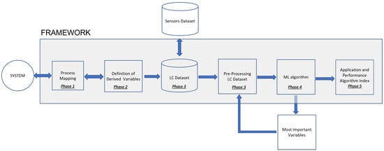
Figure 1.
Framework Flowchart.
A description of these phases is presented below.
- Phase 1: Mapping Process
Prior to the data collection phase, a set of candidate variables for critical attributes must be established, as it will be precisely the records of these variables that will compose the data to be collected, and which will be tested later in the predictive models.
The identification of these variables starts by a process mapping which includes first the identification of critical points associated with the LC and next, the set of corresponding variables representing those points. This can be done through the analysis of technical reports and documents, field visits and interviews with the team responsible for operating the system. However, for the representation of this process mapping, some type of computational tool must be used.
For this, a well-known tool, which is used in software engineering, could be employed. This is the case of BPMN—business process model and notation. This is a notation of the business process management methodology, widely used in software engineering for process modeling. The BPMN was developed by the Business Process Management Initiative (BPMI) and is currently maintained by the Object Management Group [44,45].
BPMN concepts and the computational tools incorporating these concepts were initially designed to represent business processes, in order to improve and/or automate them. However, by mapping a process, it is possible to identify critical points in the system and, therefore, the correspondent variables involved in that system. This makes this concept more comprehensive, making these tools useful for virtually any type of system and not only to improve and/or automate a process, but also to understand the relationships and variables associated with the system. This is the case with this project. In this work, the BPMN was used to map the systems under study and thus identify its relevant variables. This is similar to what [46] has done in an industrial system, where BPMN has been used to map the system, having treated manufacturing operations as process components, combined in practical process models.
It is important to note, in this case, that the LC, which will be the basis of this work for the development of predictive models, is defined by the operating time of a device between two consecutive interruptions. Thus, in addition to the mapped variables associated with this phenomenon, it is essential to monitor the LC itself, recording the time between consecutive equipment stops, which is, in fact, the main variable to be monitored. Furthermore, from this LC monitoring, other derived variables may emerge that can be useful in a predictive model and, therefore, should be considered in the next phase of this framework.
- Phase 2: Definition and Construction of Derived Variables
In this phase, a verification of the need for new variables derived from the critical variables defined in phase 1 must be carried out, and their construction must take place, if necessary.
In general, some metrics are necessary and must be constructed to complete the set of variables to be used in the model, such as: accumulated time since the last maintenance, number of cycles since the last maintenance, number of cycles per day, average time of the cycles in the period, and maximum cycle since the last maintenance.
Eventually, other variables, not necessarily derived directly from the LC, may also be useful for the modelling, such as consumption of electricity and fuel in the period, volume of inputs for equipment operation, production equipment in the period, etc.
The whole set of variables must be defined and constructed in this phase.
- Phase 3: Data Collection, Preparation, Transformation and Storage
In this phase, in addition to data collection, a task of data preparation must be developed, which fundamentally refers to what in the KDD process is called data preprocessing [47]. In the preprocessing, any noise in the data is analyzed, such as outliers or “dirtiness” in the database, as, for example, some special characters in the database, which should have a numerical value. Missing data situations are also analyzed, which is relatively common in databases, as well as inconsistent data. In the preprocessing, these situations are identified and a solution for each case is implemented. Another important part of preprocessing is the labeling of the data, which can occur when, for some reason, it is desired to put a flag in some specific examples of the database. The possibility of making some transformations in a subset of variables must also be analyzed, as is the case of data normalization [48,49] which is even indicated for some machine learning techniques. Finally, an activity that must be considered in the pre-processing is the dimensionality analysis. The dimensions of the data set must be studied, both in the number of examples and in attributes. Eventually, a reduction in data dimensionality can be applied, providing different types of gains [50,51,52,53].
Once all these activities have been completed, you will have a database with guaranteed quality, which allows the analyses to be developed to generate reliable results. Thus, the dataset can be stored using any database tool, which will complete this phase.
- Phase 4: Predictive Modeling
The predictive modeling is the central phase of the framework, and a variety of different strategies and techniques can be used here.
In this proposal, machine learning data classification techniques should be used, as the problem under study is really one of classification between a normal equilibrium situation and another one of imminent failure. The machine learning area offers different techniques and algorithms to solve this kind of problem.
The modeling process can be tailored depending on the types and volume of data available. In fact, more than one technique can be adopted in the construction of different predictive models, generating, therefore, more than one alternative to solve the problem. Thus, in each case study, a suite of techniques can be used, each with its own results, defining a scoreboard that would allow stakeholders to visualize the full set of results and thus have more robust drivers for decision making.
Classification models must be built, and a projection for some future time must be developed, in order to indicate a situation characterizing a failure or not of the equipment.
The proposal in this framework is to develop a six-step modeling process, in a structure, as shown below:
(4.1) Definition of Techniques to be employed and Data Modeling
(4.2) Algorithms Construction
(4.3) Model Training, Validation and Testing
(4.4) Model Application and First Results Analysis
(4.5) Variable Importance Analysis and Dimensionality Reduction
(4.6) Application of Final Model Results
(4.7) Visualization, Analysis and Methods Comparison
- Phase 5: Application in a Case Study
In this phase, a case study must be selected in order to allow an application of the previous phases described here. In this research, the application took place in a hydroelectric power plant, as will be seen in the next section.
4. Case Study: A Hydroelectric Power Plant
The framework proposed here was applied in a hydroelectric power plant located near the city of São Paulo, Brazil. The hydroelectric plant is called Usina Henry Borden (UHB), and is an old company, founded in 1926, but which over time has expanded and modernized its facilities, in terms of processes and equipment. One of the aspects that has been updated is the systematic data collection process for monitoring the plant’s equipment. A significant set of sensors was installed in most equipment, generating a considerable amount of data.
The plant is installed in a coastal city in the state of São Paulo, Brazil, about 60 km from the state capital. The location at sea level favors the generation of energy, since from the plateau, where the capital of São Paulo is located, there is a water reservoir that supplies the plant, with a drop in the level of the plateau to the plant of 720 m, which is fundamental in the energy generation process in hydroelectric plants, as will be seen later in the description of this energy generation process.
The installation under study has two plants, one external, with a generation capacity of 469 MW, and another underground, whose installed capacity is 420 MW, thus having a total energy generation capacity of 889 MW. The underground part is installed in the rock in a cave 120 m long by 21 m wide and 39 m high.
The external plant is made up of eight power generation units (GU), and the underground plant has six of these generator groups. Each UG is composed of a generator, powered by two turbines, which rotate by virtue of the water flow they receive from the reservoir. The flows initially pass, still at the level of the plateau, through two butterfly valves in penstocks, where they can be controlled. Then they descend the slope, reaching the turbines. Each turbine is driven by four jets of water. In total, the water flow covers a distance of approximately 1500 m.
The operation of the UHB is part of an integrated electricity generation system that is composed of four large interdependent and interrelated subsystems. The electric energy generated at the plant is passed on to the Brazilian Interconnected System, a system that distributes energy throughout the country.
Besides the sensors, UHB has already incorporated other modern instruments into its practices, such as monitoring systems and dashboards that enable managers to visualize a set of indicators of the plant’s operation. There is also an operations control center, which monitors the entire system, providing, when necessary, indications that interventions in the system should be made. It happens, however, that a good part of the parameters and metrics on which the systems are based were defined from the practice of the operation, that is, they are empirical parameters. This situation has an impact on several aspects of the plant, which, if treated scientifically, would lead to cost reductions. Note that the operation of a hydroelectric plant involves very high costs, and even a small percentage reduction can imply relevant values. The stoppage of equipment for maintenance, for example, could be minimized with the use of predictive maintenance and not preventive, as it is done today, in which the intervals between stops are fixed and empirically defined. Additionally to cost reduction, a hydroelectric plant seeks to maximize the supply of energy and this can only be achieved if, maintenance stoppages are minimized, which can be achieved with the use of more advanced data science techniques. This is the aim of this case study, which is to deal with the development of a model able to predict failures in the operation of the turbines, which would enable the implementation of a predictive maintenance program for this equipment.
4.1. Description of the Hydroelectric Power Plant and the Power Generation System
In the specific case of this application, the aim is to use data referring to the sensors installed in the plant’s turbines, which allow the monitoring of variables related to the LC of this equipment.
In order to define this LC, it is important to clarify the basic operation of a generator turbine system in a hydroelectric plant.
There are some types of hydroelectric turbines, the most common being currently the Pelton type turbine, which is the turbine used as a reference for this project.
The turbines in the hydroelectric plant are responsible for the transformation of kinetic energy into electrical energy. This occurs through a generation unit (GU), composed of a turbine-generator system. Two turbines rotate supported by an axis that has a turbine at each end and an electricity generator at the center. The same axis, therefore, is coupled to the three pieces of equipment. As the turbines rotate, the shaft rotates and causes the generator to also rotate, and through this rotating movement, electrical energy is generated. The GU is, therefore, the heart of a hydroelectric plant [54]. Thus, monitoring this process is critical to assess the timing of an interruption in operation before a failure occurs.
4.2. Load Cycle of a Turbine
The considerations in the previous section show the importance of monitoring the turbine load cycle (TLC), which can be defined as “the time elapsed between the opening and closing of valves which release jets of water, reaching the turbine blades”.
From a practical point of view, the TLC is defined by the time the turbine remains in operation, and a turbine is in operation when its corresponding GU is on. In turn, in this specific case, each GU has an 88 KV circuit breaker which, once turned on, puts the GU into operation. So, in practice, to define the start and end of a TLC, the status of the circuit breaker switch, (on or off) must be considered. When the circuit breaker is switched off, a cycle ends. Upon restart, a new cycle begins.
On the other hand, the greater the volume of water and the time that the turbine is subjected to these jets, the greater the wear and tear suffered, and the wear and tear of the equipment makes a maintenance stop necessary at a given point in time.
Therefore, whenever it is possible to predict a period in which a failure may occur, this forecast would provide an indication that before that period, a maintenance should be scheduled. With this information, a predictive maintenance process can be defined.
A predictive model with these characteristics would be an important tool for planning maintenance and operation, leading to a reduction in losses due to unscheduled downtime.
4.3. Application of the Proposed Framework
The proposed framework was applied to the case study, in order to develop a predictive model aimed at optimizing the predictive maintenance scheduling of one GU of the UHB.
The framework was followed, according to the phases defined in Section 3, which are described next.
- Phase 1: Mapping Process—Identification of Critical Variables
A mapping process was developed to represent the operation of the UHB power plant. A methodology based on BPM was applied. Figure 2 shows a mapping of the macro representation of the full process of generating energy.

Figure 2.
Full Process.
The UHB has a wide system of sensors installed in its equipment allowing the monitoring of an expressive set of variables all over the processes showed in Figure 2. Thus, among this set of variables, those related to the research problem should be chosen. In this case, the objective was to focus exclusively on the issue of the TLC, which occurs in the turbine system, but which is affected by some sub-processes of other systems. Following the directions defined in the framework, technical documents and interviews with the operation team showed that most of the critical points to be monitored were not just in the turbine system, as was expected, but an expressive number of critical points were also in the adduction system. General views of these systems are presented in Appendix A. As these systems are somewhat complex in terms of components, interrelations and numbers of variables, the purpose of the figures is really to provide just an overview of the breadth of the systems.
In the adduction system 9 variables were identified, and in the turbine system 12 variables associated with the TLC were found. Two more variables were discovered in the generator and transmission systems. In this way, a set of 23 variables monitored directly by the sensors was defined. To this original set, 3 more variables were added that reveal anomalies in the system. Once detected, they trigger system alarms, which are registered.
- Phase 2: Definition and Construction of Derived Variables
In phase 1, 26 variables were defined. To this set, another 9 variables were added, derived from data collected. These computed variables were determined through some metrics defining specific characteristics of the TLC behavior. The final set of variables was composed of 35 indicators, plus the date and time stamp of the collection of each piece of information, resulting in a dataset with 36 attributes. In this dataset, a group of seven variables associated with pressure in valves was established. There was also a pair of two variables related to water flow measurements, and another group of six variables measuring the position of the water injection needles and jet deflectors. A variable was selected to record the condition of the circuit breaker (on or off), and another one to register the active power generated. A group of seven variables measure frequencies of rotation of the equipment, and a last pair of variables that detect anomalies was defined. These are the original variables collected directly by sensors. Regarding the derived variables, a set of nine indicators was established to define metrics related to the characteristics of the TLC, and one more variable was defined to calculate a metric about the alarms. The whole set of variables is presented in Table 1.

Table 1.
Load Cycle: Critical Variables.
- Phase 3: Data Collection, Preparation, Transformation and Storage
The data in UHB are collected continuously by the sensors installed in the equipment of the plant. For the purpose of this research, a sample of a period of 16 months was selected, from June, 2018 to October, 2019. The data collection focused on one UHB generating unit (GU), known as GU6. The data were extracted from a supervisory system database fed by the sensors coupled to the plant equipment, which were connected to this system. This extraction generated the dataset employed in the analyses.
Preceding the construction of the model, the raw data were submitted to a preprocessing treatment to identify any kind of noising, including missing data, inconsistency and outliers. This preprocessing phase must always be performed when dealing with databases, and in this specific case, the following aspects were considered:
- -
- missing values, which in some cases were identified and recovered, but in others the examples could not be recovered and were then eliminated;
- -
- inconsistencies, such as finding a character in some attribute, where there should be a numerical value, which in some cases it was possible to retrieve the correct information, and in others it was not possible to do this recovery and the copy was thus eliminated;
- -
- analysis of outliers, which in some cases were errors due to malfunctioning sensors and in other cases were maintained, as they corresponded to situations of effective anomalies that were occurring in the operation;
- -
- data normalization, as some of the techniques used require this type of data processing;
A task usually developed in the pre-processing is an analysis of the attributes, checking if there is a need for a data dimensionality reduction (DDR). However, in this case, as the mapping developed had selected just a limited number of relevant variables, there was no need for DDR at this phase. Once the data were cleaned they were stored in a database and the derived variables presented in phase 2 were computed. The result was a final dataset composed of 1,406,734 examples and 36 attributes.
- Exploratory Data Analysis: Turbine Load Cycle Dashboard
Once the data preparation and transformation was done, exploratory data analysis was developed to understand the data behavior. Moreover, a dashboard was developed that may have different information and statistics, and can be used to monitor the processes by the operations team.
Figure 3 presents an example of some statistics for a specific period, as an illustration of this process.
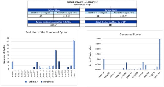
Figure 3.
Turbine Load Cycle—General Dashboard for a Period—EXAMPLE.
- Phase 4: Predictive Modeling
Once the data quality was assured in phase 3, the modelling phase took place, and the six steps defined in Section 3 were followed, namely: the definition of techniques to be employed and data modeling; algorithm construction; model training, validation and testing; results analysis, variable importance analysis and dimensionality reduction; final results visualization and analysis.
- Step 4.1: Data Modeling and Methods Explored in the Predictions
Before defining the methods to be used, it should be considered that regardless of the technique, there is an essential issue that is the approach to building the predictive model, since the same dataset and the input variables of a model can be used and modeled in different ways, depending on the strategy of construction and, eventually, even the set of variables can be changed depending on the approach.
In a first approach that could be considered, a predictive model can be defined in such a way that the prediction of the optimal time of shutdown for maintenance can be predicted from a single variable, an alarm, for example, that indicates a degradation effect of a piece of equipment. Projecting this variable into the future would lead to a prediction of when an interruption of the operation should occur and, therefore, maintenance is scheduled for some time before this predicted occurrence.This could be a classic time series analysis and forecasting approach.
Another approach to consider would be to work with two predictive models. A first mathematical model must represent a relationship between variables (explanatory attributes), which would be causes of wear, and the occurrence of failures in future periods (dependent variable). There must also still be a second model to project these explanatory variables for future periods, being able to identify, when applying the first model, a time horizon in which a failure should occur. Note that this is an approach that requires the projection of a set of variables, not just one. These projections must be able to predict non-standard values of these variables, and not just average values or trends, as it is the outliers which, in general, indicate equipment failure trends. Thus, there is a predictive modeling task that is not trivial.
A third approach would be to consider a set of variables that may indicate future failures, as in the second strategy, but without the need to create mathematical relationships between the dependent variable and explanatory variables. In this case, you must have a historical database that stores values collected from these variables with the respective timestamps of data collection. From these data, it is possible to identify for each instance (each example) the occurrence or not of a failure in fixed time horizons, defined as time intervals from the instant associated with that instance. With this, it is possible to build a data modeling and a predictive model which, considering only the current conditions of these variables, would be able to project the occurrence of a failure in the considered time horizons. In this case, a time series forecasting problem, mainly based in regression models, is transformed in a data classification problem. The research presented here adopted the latter approach, as detailed below.
- Step 4.1.1: Data Modeling for Predictions
The data modeling needed to be constructed in a way that allowed the transformation of a time series forecasting problem into a data classification problem. It was assumed, therefore, that the approach to be adopted in modeling would be the use of supervised ML techniques. Data modeling, therefore, should be appropriate for this paradigm.
For this, we started from the premise that it would be important to have at least 12 h in advance, a prediction that an equipment failure could occur. Thus, the final modeling considered predictions for 12 h and also 24 h and 48 h in advance.
The data should be modeled for this strategy. Therefore, new labels were created to identify occurrences that could generate a failure alarm in the future periods of 12, 24 and 48 h.
For this, an algorithm was built to identify all failure alarms registered in the data set, which is represented by the variable number 36, and their date and time, correspondent to the variable number 01, timestamp.
Initially, three new fields were created in the database, as shown in the Table 2.
Table 2.
Load Cycle: NEW ATTRIBUTES (LABELS).
Subsequently, the dataset is sorted in descending order by date/time, and a search is started from the first record, looking for records that indicate the occurrence of an alarm. Once the record of the first alarm is found, a new search is made, based on the date/time information, to find the first record with a date/time before that alarm whose time interval is greater than or equal to 12 h. This first record found is labeled with a 12-h flag (variable t12 = True). This routine is applied to all records in the database and, once completed, it is repeated considering the intervals of 24 and 48 h (variables t24 and t48).
With this data modeling, the dataset was prepared to deal with a data classification problem, and a suite of machine learning techniques was applied to the transformed dataset, as showed in the following.
- Step 4.1.2: Methods Selected for Predictions
Regarding the methods selected for the prediction models, it should be considered that one of the objectives of the paper was to verify whether it would be feasible to apply ML to the data of the specific problem at hand. There are references in the literature about the use of ML in PdM, but there is a gap in relation to the specific problem of a hydroelectric power plant. There are many references dealing with wind power plants, but not with hydroelectric power plants. Thus, it was necessary to verify if ML could adapt well to the data to predict equipment failures of this other type of power plant, and for that it would be necessary to test some ML methods.
The objective, therefore, was to apply ML techniques, and demonstrate that PdM related to a key subsystem of a hydroelectric power plant could benefit from the algorithms of this area of knowledge.
In this sense, it was necessary to select classic ML methods that were representative of ML algorithms and that had different complexity and characteristics. Thus, three methods were initially chosen that met these criteria: decision tree (DT), artificial neural network (ANN) and logistic regression (LR).
DT has a structure based on logical rules distributed in a hierarchical flowchart-like tree structure, and is a “white box” algorithm, which generates a model that is a set of logical rules [55].
ANN works with a somewhat complex mathematical model involving different learning strategies, a network of neurons (nodes) connected by links (synapses) in multiple layers, link weights, various types of hyper-parameters, and functions of different types, and is a “black box” model with high complexity [56].
The third technique chosen, LR, is a particular case of the generalized linear models (GLM). Proposed by [57] and reintroduced by [58], it is an extension of the linear model based on the normal distribution. LR classifies data by determining probabilities [59], which in turn are determined through regression equations, whose parameters are estimated by well-known classical statistical methods. These three methods, with very different characteristics and different levels of complexity, could lead to different levels of accuracy and performance of the models. To complete this picture, a fourth approach based on a composition of models was included (an ensemble), for which the RF [60] was selected, a traditional technique that is widely used in many types of applications.
Therefore, a set of four methods was consolidated to be applied to the dataset.
This set of varied techniques, representative of different ML algorithms, made it possible to evaluate the feasibility of applying ML to the data. If some or all of them were reasonably accurate, this could be interpreted as an indication that ML could be applied to this type of data/problem.
To shed a little more light on the selected methods, it is worth saying that decision tree is a classical data classification technique and it is possibly the most used algorithm for classification. Eventually, it could be said that this would be a technique that at least deserves to be explored whenever you have a data classification problem.
Artificial neural network (ANN) is another classical machine learning technique often used for data classification. It is versatile, being able to be used in different types of problems, and many times presents a performance at the highest level.
Logistic regression is a method that seems to be perfectly suited to the type of problem being studied. Regression defines a relationship between a dependent variable and one or more independent variables, which would explain the behavior of the first variable. When the dependent variable is binomial, there is the case of a logistic regression, which is specifically the situation of the present study.
Finally, random forest is the case of an ensemble method, which is a composite of multiple models. This is a different strategy from the previous techniques and, therefore, it is an alternative that deserves to be considered among the tested approaches. Specifically, the random forest is a set of decision trees and is, therefore, well suited to the problem under study.
- Step 4.2: Algorithms Construction—Classification Models
At this stage, the data classification techniques were implemented to classify the examples into two categories: normal situations and imminent failure situations.
The classification models were built based on the algorithms presented in the prior step. The implementation was carried out in the environment of the R programming language and the R Studio tool, and making use of R libraries, which are available in more than one version, for all tested algorithms and for the development of predictions and indicator generation, which were used to evaluate the models. For the training of the models and for the validation and testing phases, resources from the R programming language environment were also used, as explained in the following.
For the implementation of the DT model, the library “rpart—Recursive Partitioning and Regression Trees”, for the R language environment was used [61], which is an implementation of the main functionalities of the 1984 proposal by [60]. The implementation of the model, was done with the “rpart” function. The main parameters, which provided the best results, are presented below:
. method = “class”: specifies a classification problem
. minsplit = 1: minimum number for split in a node
. split = “Information”: specifies the criterion on which attributes will be selected for splitting.
The entropies of all attributes are computed and the one with the least entropy is selected for split.
. Default parameters having been used in all other arguments.
As a criterion for evaluating the model for the purpose of its construction, the metric of “information gain” was used.
Regarding the MLP network, the implementation was possible through the package RSNNS, which is implemented in R, the library SNNS (Stuttgart neural network simulator) [62], which is a library containing standard implementations of neural networks. By this package, the most common neural network topologies and learning algorithms are directly accessible by R, including MLP. For the implementation of the model, the “mlp” function was used. The list of the main arguments, which enabled the best results, is presented below:
. MLP, which is a fully connected feedforward network
. Two hidden layers
. First layer with five neurons and the other with seven neurons
. Standard backpropagation
. Random weights for network initialization
. A logistic activation function
. Learning rate = 0.1
. Maximum number of iterations = 50
. Default values for the rest of the parameters.
In the case of LR implementation, the function “glm” was used, which is a native function of R, aiming to fit generalized linear models to the data, providing a symbolic description of the linear predictor and a description of the error distribution. The main arguments, which generated the best performance indicators, are presented below:
. Error distribution (family) = binomial, which provides a logistic regression model
. method = iteratively reweighted least squares (used in fitting the model)
. intercept = True (include an intercept)
. Default values for all other parameters
For the implementation of the RF algorithm, the package “randomForest—Breiman and Cutler’s Random Forests for Classification and Regression” was used [63,64], which is offered for use in the R environment, and which uses random inputs, as proposed by [60]. The model itself was built with a function from this library, with the same name as randomForest. As for the main arguments, which provided the best results, their list is presented below:
. Number of trees to grow (ntree) = 200
. Number of variables randomly sampled as candidates at each split (mtry) = square root of the number of variables (default)
. cutoff = 1/(number of classes) The ‘winning’ class for an observation is the one with the maximum ratio of the proportion of votes to cutoff (in this case, majority vote wins)
. Minimum size of terminal nodes (nodesize) = 1 (Default)
. Maximum number of terminal nodes trees (maxnodes) = Subject to limits by nodesize
. Default values for the other arguments.
- Step 4.3: Model Training, Validation and Testing
Regarding the training of the models used in this study, a resampling process was adopted.
There are several resampling techniques, which basically subdivide the data into learning and testing sets, and can vary in terms of complexity [65]. One of the best techniques to verify the effectiveness of a machine learning model is the K-fold crossvalidation, which was used here. The parameter k represents the number of folders (samples) to be created for training, validation and testing. In this study, the value of K = 5 was used. Thus, four folders (80% of the data) were used to train and validate the model, and one of them (20% of the data) to perform the final test of the model. This parameterization proved to be adequate for conducting the experiments, having generated results with high accuracy.
The four folders (samples) were selected by random sampling, and as the model is applied to the examples of each folder, its hyper parameters are adjusted. Once these parameters are properly calibrated, the model is then applied in the folder dedicated to the final test.
For the training and testing of the models with the cross-validation technique, the library “cvTools—Cross-validation Tools for Regression Models” [66] was used, which offers tools in the R environment for the application of this technique. For all models, the proportion of 80% of the data for training and 20% for tests was maintained.
- Step 4.4: Model Application and First Results Analysis
The four models described in step 4.1 were applied to the dataset in order to predict a failure in the equipment in a period of 12 h, 24 h and 48 h.
In a first approach, the models were applied to the data considering all attributes of the database as explanatory variables.
The performance was evaluated initially through a confusion matrix [67], which is particularly indicated to classification procedures where there are two possible states: TRUE or FALSE.
The structure of a confusion matrix is presented in Table 3.
Table 3.
Confusion Matrix.
For this matrix we have:
TP = Number of True Positive Cases
FP = Number of False Positive Cases
FN = Number of False Negative Cases
TN = Number of True Negative Cases.
TP are the cases for which the actual class of the data was TRUE and the model predicted TRUE (correct). FP, on the other hand, are the cases when the actual class of the data was FALSE but the predicted was TRUE (incorrect).
FN measures incorrect FALSE predictions. These are the cases when the actual class of the data was TRUE and the predicted was FALSE (incorrect). Finally, TN are the correct predictions for FALSE cases. The cases where the actual class of the data was FALSE and the classifier predicted FALSE (correct).
In the experiments carried out in this research, it was considered that an Actual Positive condition of the system was TRUE when an Alarm occurred in an period of 12 h or less, or 24/48 h if these were the time intervals considered. On the other hand, the TN counter was increased by one each time a normal prediction was correct.
The confusion matrix is not a complete performance metric in itself, but most KPI‘s (key performance indicators) used to evaluate models are based on this matrix, see [68,69,70].
In this experiment, a set of KPI‘s were utilized, which are generated by a package available in the R language, called caret (classification and regression training) [71], which computes a set of indicators from a confusion matrix, as described below:
. Accuracy (Acc), which shows the proportion of classification performed correctly, that is, TP + TN as a proportion of the total classified items.
. Precision or positive predictive value (Pos Pred Value), that is a proportion of cases predicted as TRUE that were really TRUE.
. Negative predictive value (Neg Pred Value), presents the number of negative class correctly predicted as a proportion of the total negative class predictions made.
. Sensitivity or recall, a proportion of cases classified as TRUE over the total TRUE cases.
. Specificity, which represents the proportion of cases classified as FALSE over the total FALSE cases.
. Prevalence, which presents the total actual positive classes as a proportion of the total number of examples.
. Detection rate, corresponds to the true positive class predictions as a proportion of all of the predictions made:
. Detection prevalence, corresponds to the number of positive class predictions made as a proportion of all predictions:
. Balanced accuracy, corresponds to the average between sensitivity and specificity.
- . Non-information rate (NIR)
This is the accuracy that would be achieved simply by always predicting the majority class [72]. It is a good KPI to compare against calculated accuracy.
- . Acc vs. NIR—hypothesis test (p-value)
This is an one-sided hypothesis test to see if the accuracy (Acc) is better than the “No Information Rate (NIR)”.
The null hypothesis (Ho) of the test is presented below:
Ho: Acc ≤ NIR
For a p-value ≤ 0.05, Ho can be rejected.
- . Kappa coefficient
The Kappa coefficient, discussed in [72,73], is considered a standard for assessing agreement between rates. The calculation is made considering the rates observed in an experiment versus the rates that would be expected due to chance alone.
In terms of confusion matrix, it is a measure of the percentage of values on the main diagonal of the matrix adjusted to the volume of agreements that one could expect as a function of chance alone.
Kappa ranges between 0 and 1.0, and when K is within the range 0.6 < K < 0.8, indicates substantial agreement.
The Kappa coefficient is computed through the formula below;
where:
= Observed probability (percentage);
= Chance probability (percentage).
- . McNemar Statistic Test
This test [74] is applied to a contingency table, similar to a confusion matrix. This tests a null hypothesis of marginal homogeneity that states that the two marginal probabilities for each outcome are the same, i.e.,
where:
Thus, this can be synthesised to the following null hypothesis:
The McNemar test statistic is given by:
We can reject Ho, if the p-value for the test is less than 0.05.
With this last statistical test, the set of metrics used in the analysis of the results generated by the models was consolidated.
In addition to analyzing the performance of the models, it should be considered that in data mining, the input variables of the model hardly have the same relevance [75]. In most cases, only a part of these variables really contributes to explaining the dependent variable. Thus, it is important to identify the most important variables because, in this way, it is possible to reduce the dimensions of the problem, reducing the complexity of the model and, consequently, requiring less computational resources.
In this research, a first round of executions of the models was carried out, which allowed the identification of the most important variables (MIV) in each model. Then, in a second round of experiments, only the MIV of each technique were considered, applying, therefore, a data dimensionality reduction.
After this second stage of applying the models, a panel of metrics (tables and graphs) was developed to assess the accuracy and significance of the results, in order to allow a clearer visualization of those results generated by each model developed.
- Step 4.5: Variable Importance Analysis and Data Dimensionality Reduction
The importance of a variable could be described, more generally, as the level of impact that this variable has on the outcome of the response variable. This can be represented as a value. So, variables with a greater importance value (IV) would have more impact in an expected outcome.
In this paper, the IVs were computed for all variables in the models, and sets of 10 MIVs were identified for each one of the prediction models and for each of the time horizons considered: 12 h, 24 h and 48 h prediction.
Next, the common top 10 variables to the three time horizons for each technique were identified. Each set of common MIV then became a number greater than or equal to 10 variables.
Thus, for each type of model, the following results were obtained:
. DT Model: 14 MIV;
. MLP model: 17 MIV;
. LR model: 18 MIV;
. RF model: 12 MIV.
These MIVs are presented in Table 4.
Table 4.
MIV per Model Type.
One aspect that is important to explain about the IV calculations is that each model/ technique has its own procedure for determining IV.
These procedures, which are used in the techniques applied in this paper, are presented below.
- Importance Values Computation for Decision Trees and Random Forest
In decision trees, the attribute chosen for each node of the tree is defined so that it maximizes the chosen metric to provide a gain in the accuracy of the results. Thus, the relative importance of a given variable (or attribute) is defined as the sum of the quadratic gains of all nodes in the tree where that variable was chosen to define the partitioning of the instances that pass through the node. This same concept can be extended to one or more sets of decision trees, as is the case with random forests [76].
- Importance Values Computation for Artificial Neural Network
In this work, a proposal developed by [77] was used. In this method, the weights of the connections between the layers of a neural network constitute the basis for establishing the values of the VI. The method calculates the importance of a variable as the product of the weights of each input and output connection of all neurons, of all hidden layers of the network, and sums all these products. An advantage of this approach is that the relative contributions of each weight of a link are considered in terms of magnitude and sign. Thus, in a case where the weights change sign (positive to negative or vice versa) between the input and output layers, these would have a cancellation effect. Other algorithms can give misleading results by considering only the absolute magnitude. Another additional advantage is that the [77] is able to assess neural networks with many hidden layers. It should be noted, however, that the values of the importance attributed to the variables are measured in units based directly on the summed product of the connection weights of the specific neural network model under analysis. Thus, these values should only be used in terms of sign and magnitude as a standard for comparing the explanatory variables of the model being analyzed. Comparisons with other models can lead to misunderstandings [78].
- Importance Values Computation for Logistic Regression—LR
In linear models, the absolute value of the t-statistic or equivalent is usually used as a measure of variable importance [76]. The t-statistic or equivalent is related to the null hypothesis (Ho) tested in a linear model. This hypothesis, Ho, states that the coefficient of an explanatory variable would be zero (Ho: = 0). The larger the value of t or equivalent, the smaller the p-value, which is the P(Ho = True), and which means that we should reject Ho, for very small p-values. Therefore, using the t-statistic as a measure of VI is a criterion that makes sense, because the larger the t-value or equivalent, the smaller is the p-value, and, consequently, the more significant is the correspondent variable. The same concept extends to the case of generalized linear models (GLMs), used in this work for the construction of the logistic regression models. In the LR models developed in this work, the R language library used for the VI calculations generated values that exactly coincide with the Z value generated in the statistical analysis of the model.
In this article, the determination of MIV and its respective IV’s were developed through an R language library, called “vip” (variable importance plot) [76], which applies all these concepts that we have just seen, computing the IV of each variable.
The Table 4 presents the MIV for each model.
Figure 4, Figure 5, Figure 6 and Figure 7, show for each type of model the MIV’s and their respective IV’s. Each figure presents three graphics showing the IV’s for the three time period predictions considered in the study: 12-h, 24-h and 48-h.
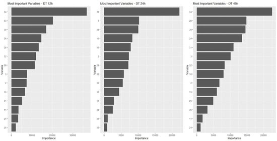
Figure 4.
Most Important Variables for DT—Decision Tree Models.
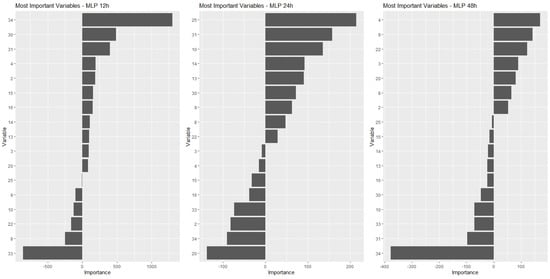
Figure 5.
Most Important Variables for MLP—Multilayer Perceptron Models.
Figure 6.
Most Important Variables for LR—Logistic Regression Models.
Figure 7.
Most Important Variables for RF—Random Forest Models.
By observing these graphs, it can be seen that the best ranked variables have IV’s much higher than those at the bottom of the list. However, given the shape of the curves, it could not be said that this decrease is linear. Note that there is a certain stabilization or small reductions in the IV for variables positioned towards the end of the ranking, which means that there is not much difference in the importance of these variables. It is possible, eventually, to use one or another variable without much difference in the results obtained. On the other hand, if any of the variables from the beginning of the ranking are not included in the model, the impacts on the results can be significant, given the relative magnitude of their IV’s. This behavior could lead us to think of a decrease in IV associated with the inverse of a power curve.
- Global Most Important Variables
In addition to determining the MIV’s for each type of model, it would also be important to establish the most important variables globally, considering the entire set of models developed, thus defining a global ranking of variables.
In order to develop this ranking, two types of weights associated with the importance of the variables were defined, and a final weight was determined through a combination of these two weights.
The first of these weights () set a numerical value for each time a variable appeared in the list of MIV. As four modeling techniques were used, the number of times a variable could appear would vary between 1 and 4 and, therefore, the relative weights that were adopted () range from 0.25 to 1.0.
A second weight () was defined based on the position of the variable in the MIV ranking. These weights, therefore, should be inversely proportional to the variable’s rank.
To establish the inverse relationship, a regression model was estimated to represent the normalized mean IVs of the variables in the model set, as a function of the positions of the variables in the ranking of importance.
The process of determining these weights, therefore, started with the normalization of the IVs of the variables in each model, and then a general average of these normalized values was computed for each position of the ranking, considering all the developed models.
The IVs were normalized using Equation (4):
where
= normalized of variable i, of model j
= of variable i, in model j
= maximum observed of the variables in the model j
= minimum observed of the variables in the model j
i = 1, 2, ..., ; j = 1, 2, 3, 4
= number of MIV in model type j.
This normalization was carried out for the 12 models developed: four types of models, with three forecast time horizons, 12 h, 24 h and 48 h. Then, the averages of the 12 models of the normalized IVs of each position in the ranking were computed.
As the number of MIVs in each type of model was not the same, the averages were computed so that there were always 12 observations in the calculation of each average.
For this criterion to be met, the means were computed up to a number m of MIVs, where
With this procedure, a vector of average normalized IVs was generated. This vector allowed the representation of the average normalized IVs as a function of the positions of the variables in the ranking of importance.
A regression model to represent this relationship was then developed, presented in Equation (6), which obtained a coefficient of determination () of 0.9843. The normalized values estimated through this model were adopted as the second weight () associated with the MIVs ranking.
where:
= weight 2, associated with the MIV rank
r = position of the variable in the MIV ranking.
Regarding this Equation (6), it should be remembered that it must be fitted to the data of each application.
Graphically, a normalized mean curve of the observed IVs and the respective curve adjusted to the data is presented in Figure 8.

Figure 8.
IV = f(r)—Normalized Mean Curve.
Through Equation (6) the weights of each variable were estimated. As in the case of the first weight (), here too, a relative weight was computed. By the model (6), the of a variable positioned in the first place of the ranking (r = 1) would be 0.9858. Now, considering the four models developed, the maximum sum of would be 4 times 0.9858, or 11.8, which we rounded to 12. Having this total maximum absolute value as a reference, the normalized IVs of each variable in the models were added and divided by 12, generating a relative weight () for each variable.
The final global weight of each variable corresponds to the multiplication of the two weights, as shown in Equation (7):
The Table 5 shows the weight compositions for all variables.
Table 5.
Most Important Variables—Weights Composition.
The relevance of these global MIVs is that this finding can be a reference for the selection of variables for predictive models in new applications.
Table 6 shows the final global weights and the final global ranking of the variables.
Table 6.
Final Ranking of Global Most Important Variables.
It should be noted, from Table 6, that of the first five most important variables, four are related to times and amounts of charge cycles, and one is related to valve pressure.
Thus, in view of these results, and in order to seek a reduction in the dimensionality of the data, it was decided to work only with the MIVs, thus reducing the computational and analysis effort, without compromising quality, and new experiments were performed only with the MIVs. The complete set of results obtained in the experiments are presented in the next step 4.6.
- Step 4.6: Application of Final Models Results
Table 7, Table 8 and Table 9 show the results of experiments considering the entire set of variables (All Variables) and only the most important variables (Top Variables). The results obtained in these experiments with the Top Variables remained at the same level as those generated with the full set of variables, and in some cases, were even better.
Table 7.
Methods Comparison by Key Performance Indicators: Alarm Prediction in 12 h.
Table 8.
Methods Comparison by Key Performance Indicators: Alarm Prediction in 24 h.
Table 9.
Methods Comparison by Key Performance Indicators: Alarm Prediction in 48 h.
In relation to these results, most of the KPIs showed reasonably robust results, not significantly differentiating the four models explored in the experiments. In this set of KPIs with robust values, the accuracy in particular, which, as a rule, is one of the most used metrics, was very high in all tests of all models. If the analysis was based on this set of KPIs with robust values, there would be some difficulty in differentiating the models. Looking only at this set of KPIs, it could be considered that all models are reasonably robust. There is practically no difference between the results. There are, however, five KPIs that stand out from the others, showing important differences between the models. Although, of these five, there are four that effectively differ, because two of them, Balanced Accuracy and Specifity, are related to each other.
A visualization of this Final Global Rank is shown in Figure 9.

Figure 9.
Final Ranking of Global Most Important Variables.
Therefore, the final group was left with four KPIs, and we named it Key Analysis Points (KAP), which are presented below:
. P[]
. Kappa coefficient
. Negative predicted value
. Specificity
When considering this specific KAP, the picture changes considerably and it is possible to identify performance differences between the models, which draws our attention to the importance of analyzing the results from different angles.
- Step 4.7: Visualization, Analysis and Methods Comparison
A visualization of the KPIs for the three time horizon of predictions can be seen in Figure 10, Figure 11 and Figure 12. The figures present the KPIs computed for the models with “all variables” (All) and for the models with only the MIV. Moreover, for each time horizon, there are two graphics: the first one considering the set of KPIS with robust values for all four models, and a second graphic with the set of KAP, the key analysis points, which are the KPIs with a significant variation between the models. These figures provide a clear comparison between the methods.
Figure 10.
Methods Comparison by KPIs for Alarm Prediction in 12 h.

Figure 11.
Methods Comparison by KPIs for Alarm Prediction in 24 h.
Figure 12.
Methods Comparison by KPIs for Alarm Prediction in 48 h.
From this group of Figure 10, Figure 11 and Figure 12, it appears that there are important differences between the methods, but that these differences are only shown by a restricted group of indicators.
The DT and RF models both had satisfactory KPIs in all experiments, but this was not true for the other models. In some cases, the KPIs indicate that the model should in fact be discarded, as the KPI result showed that the results obtained with that model lacked significance.
The models that did not show satisfactory results for this KAP group of KPIs were the logistic regression (LR) model and MLP (multilayer perceptron). In these two cases, the behavior of the KPIs was different depending on the time horizon of predictions: equipment failure in 12 h, 24 h or 48 h.
By analyzing the indicators and graphs, it can be seen that the regression modeling was not able to capture the behavior of the data as well as other models. This can be seen specifically by the indicators:
. P [];
. Kappa coefficient;
. Negative predicted value and
. Specificity.
The same can be said about MLP. It was not possible to get to a model based on MLP that would lead to results of the same level obtained with DT and RF, and the model runtime is also an issue. While some models reach the solution in seconds, the MLP took more than 1 h. On the other hand, the DT and the ensemble, RF, found logical rules in the database, which led to results with high values for all indicators and with the advantage of having low execution times.
For the 12 h predictions, the kappa coefficient had a value below 0.5 for the LR, which is not a satisfactory result, and this happened both for the “All Variables” experiments, as in the case of “Top Variables”. The kappa coefficient, as mentioned before, is considered a standard to assess agreement between rates. In our case, it measures the hits that could be expected in the confusion matrix as a function of chance alone. A value above 0.6 would indicate a good quality of the model’s response. The closer to 1, the better the prediction.
Another situation in the 12 h prediction happened with MLP which gave a value for the negative predicted value below 0.6 in both cases: all variables and top variables.
When checking the results of the 24 h predictions, MLP and LR again did not show satisfactory responses for some KPIs. In the case of MLP, we had NIR > Acc in both types of experiments, which resulted in a P[] = 1.0. The kappa coefficient was 0.4865 for all variables and 0.1833 for top variables. The negative predicted value was 0.4194 for the all variables experiment and 0.1045 for the top variables experiment. In the case of LR, the results were very similar, and still had very low values for the specificity coefficient and negative predicted value.
The 48-h predictions presented results very similar to the 12-h ones, for all KPIS mentioned: NIR, the p-Value [], specificity and negative predicted value, for both MLP and LR, and in both experiments: all variables and top variables.
Another way to see this difference in KPI values between the models is to analyze the coefficient of variation (CV) for each KPI. CV is the standard deviation divided by the mean value of the KPI in the four models. It represents the standard deviation as a proportion of the mean. A visualization of the CVs, for the three time horizons of predictions, can be seen in Figure 13, Figure 14 and Figure 15.
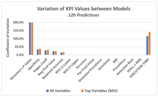
Figure 13.
Variation in KPI Values between Models expressed by CV—12 h Predictions.

Figure 14.
Variation in KPI Values between Models expressed by CV—24 h Predictions.
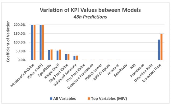
Figure 15.
Variation in KPI Values between Models expressed by CV—48 h Predictions.
From these last Figure 13, Figure 14 and Figure 15, which present KAP, it appears again that there are important differences between the models, but that these differences are only shown by a restricted group of indicators.
In particular, these last figures show that while for some KPIs, there is a high level of variation between the models, for others, the variation, expressed by the coefficient of variation (CV), is very close to zero, meaning that in all models, those KPIs got to almost the same value (almost no variation, at all).
The variation implies that, for some models, the value of the KPI is high, while for others it is low, meaning that the models with low KPI values did not achieve a consistent prediction, which confirms the conclusions obtained from the previous Figure 10, Figure 11 and Figure 12.
As a summary of these analyses, there are, therefore, results that could be considered satisfactory, particularly for the DT and RF models, given the KPIs’ presented high values in all tested conditions.
On the other hand, in the case of MLP and LR, a set of KPIs showed good results, but other KPIs did not. This happened precisely with the important KPIs such as p-Value [Accuracy ≤ NIR], and also with the kappa coefficient.
Regardless, the objective of showing that ML algorithms could be employed for PdM in a hydroelectric power plant environment was achieved for at least two of the algorithms tested.
Finally, these analyses of results confirm, as mentioned earlier, the importance of not considering only a few KPIs to analyze a model, as, for example, only those coefficients that revolve around accuracy, such as specificity, sensitivity and others. The indicators that provide greater statistical significance to the results are also fundamental in these analyses of the prediction model responses.
5. Conclusions and Future Work
This study sought to present a process that could be considered broad, or close to it, for the construction and validation of a predictive model of equipment stoppages due to operational failures. The model should be built using machine learning techniques, and should be used in predictive maintenance planning processes.
The process developed to achieve this proposal constituted a framework that ranges from data collection, through to pre-processing, choice of modeling techniques and tools, and the construction, testing and validation of models in a real concrete case of an industrial facility.
The research question and the objectives of the work, at the beginning of this article, pose the challenges that the research proposed.
In this research question, the first part asked about the feasibility of developing a predictive model based on variables associated with the LC of industrial equipment. On this point, it can be said that this feasibility was demonstrated in the study. The four constructed models were effective in predicting equipment failure in future periods of 12 h, 24 h and 48 h, as demonstrated by the KPIs used in the study, with two of these models having better results than the others.
There is a second part of the research question about the definition of the phases of the methodology, techniques, and algorithms, and also the variables to be considered in the model. The proposed framework has consistently contemplated answers to all these points.
Strategies and techniques were also developed to train, validate, and reduce the dimensionality of the models, and apply them in a concrete practical case of the real world in an industrial environment. Thus, all the items of the objectives outlined at the beginning of this article were achieved.
As additional contributions of this study, there was also the study of the IVM, which was important for clarifying a question that usually arises, which is the identification of the most relevant attributes of a data set. This study offers a contribution by showing how the IV is determined in different types of techniques and indicating tools for the computation of the values of this importance.
It also shows that this is an agile way to reduce the dimensionality of a dataset, working with just the MIV in the models. In the study, the impact of reducing the quantity of attributes on the effectiveness of the models was practically nil, as the results obtained in the reduced models were basically the same, as shown by the indicators.
Thus, it can be said that the main conclusions of this study, which also reflect their contributions, could be expressed as follows:
(a) The proposed framework consistently contemplated answers to all the challenges proposed in the study, ranging from the mapping of processes, through to the definition and construction of variables derived from the original collected variables, the collection, preparation, transformation and storage of the data, and the predictive modeling and application of the models to a real-world case.
(b) Four predictive models were developed, which were effective in predicting equipment failure in future periods of 12 h, 24 h and 48 h, as demonstrated by the indicators used in the study, having developed effective strategies and techniques to train and validate the models.
(c) Extensive work was also carried out aimed at analyzing the results of the models through a set of indicators, showing that the use of indicators that present different angles of the results is essential for validating models.
(d) As additional contributions of this study, there was also the study of the most important variables—IVM, which was important for clarifying a question that usually arises, which is the identification of the most relevant attributes of a data set. Here, a contribution was made with a presentation of how the importance of a variable is determined in different types of techniques. There was also the development of a global indicator of importance of the descriptive variables of the models, passing through the set of techniques used. The idea of this indicator can be adopted for other types of techniques and problems.
(e) The MIV were the basis for reducing the dimensionality of the data and, together with the set of indicators used to assess the models and with the applications in a concrete practical case in the real world in an industrial environment, it was possible to demonstrate the effectiveness of this dimensionality reduction process.
Therefore, this work brings some contributions that seem to be relevant to the topic of predictive maintenance through machine learning techniques.
There are, however, new advances that can be pursued in future work. Among the possible alternatives for new work, one can think of:
- -
- applying the models developed in other databases;
- -
- testing new approaches such as, for example, SGTM;
- -
- applying the framework in a different industrial context, which would require new models to be developed.
Author Contributions
Conceptualization, A.R.d.A.V.F. and L.A.d.S.; methodology A.R.d.A.V.F., L.A.d.S., M.V.B.d.A.V. and D.F.M.; software, M.V.B.d.A.V. and D.F.M.; validation, A.R.d.A.V.F. and L.A.d.S.; formal analysis A.R.d.A.V.F., L.A.d.S. and M.V.B.d.A.V.; investigation, M.V.B.d.A.V. and D.F.M.; resources, L.A.d.S. and L.S.d.S.; data curation, D.F.M. and M.V.B.d.A.V.; writing—original draft preparation, A.R.d.A.V.F., L.A.d.S. and M.V.B.d.A.V.; writing—review and editing, A.R.d.A.V.F., L.A.d.S. and M.V.B.d.A.V.; visualization, A.R.d.A.V.F., L.A.d.S. and M.V.B.d.A.V.; supervision, A.R.d.A.V.F.; project administration, A.R.d.A.V.F.; funding acquisition, L.S.d.S. All authors have read and agreed to the published version of the manuscript.
Funding
This research is a part of the R&D project “EMAE–ANEEL-P&D 00393-0008/2017”, funded by EMAE—Metropolitan Company of Water & Energy, of the state of São Paulo, Brazil.
Institutional Review Board Statement
Not applicable.
Informed Consent Statement
Not applicable.
Data Availability Statement
Not applicable.
Acknowledgments
We thank all the EMAE staff who participated in the R&D project “EMAE—ANEEL-P&D 00393-0008/2017”, and all the faculty and student members of the BigMAAp research lab at Mackenzie Presbyterian University.
Conflicts of Interest
The authors declare no conflict of interest. The funders had no role in the design of the study; in the collection, analyses, or interpretation of data; in the writing of the manuscript, or in the decision to publish the results.
Appendix A
This appendix presents, on the following pages, overviews of the mapping of the adduction system and the turbine system, showing their main components and their interrelationships.
It should be considered that these systems have a high level of complexity, with many components, interrelationships between these components and a considerable number of variables.
Therefore, the purpose of the mappings presented in the following pages is to provide an overview of the magnitude and complexity of these systems.
Figure A1.
Adduction System Mapping—Overview.
Figure A1.
Adduction System Mapping—Overview.
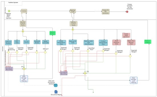
Figure A2.
Turbine System Mapping—Overview.
Figure A2.
Turbine System Mapping—Overview.
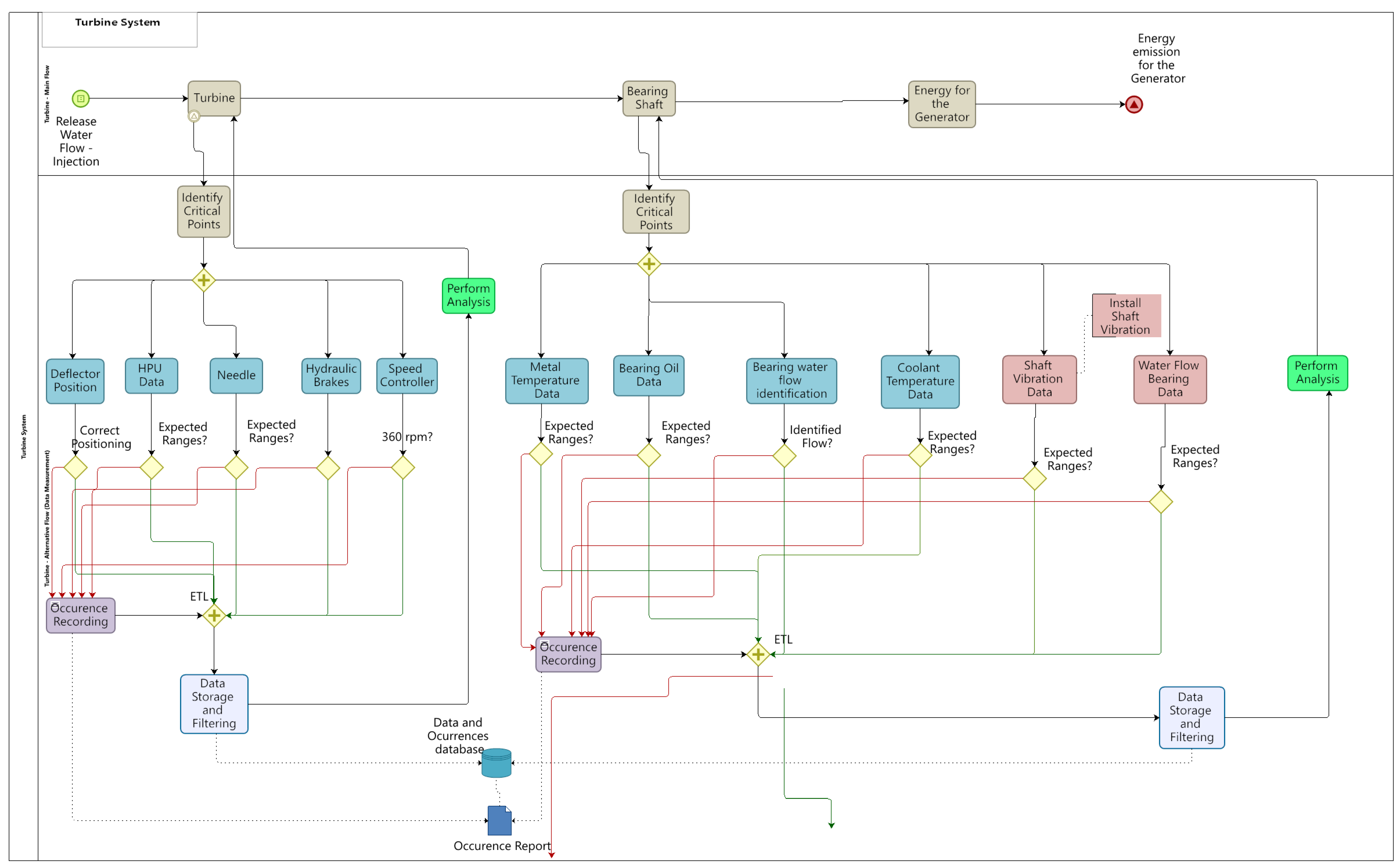
References
- Rauch, E.; Linder, C.; Dallasega, P. Anthropocentric perspective of production before and within Industry 4.0. Comput. Ind. Eng. 2020, 139, 105644. [Google Scholar] [CrossRef]
- Marjani, M.; Nasaruddin, F.; Gani, A.; Karim, A.; Abaker, I.; Hashem, T.; Siddiqa, A.; Yaqoob, I. Big IoT Data Analytics: Architecture, Opportunities, and Open Research Challenges. IEEE Access 2017, 5, 5247–5261. [Google Scholar]
- Candanedo, I.S.; Nieves, E.H.; González, S.R.; Martín, M.T.S.; Briones, A.G. Machine learning predictive model for Industry 4.0. In Proceedings of the 13th International Conference on Knowledge Management in Organizations—KMO 2018: Knowledge Management in Organizations, Žilina, Slovakia, 6–10 August 2018; pp. 501–510. [Google Scholar]
- Hernavs, J.; Ficko, M.; Berus, L.; Rudolf, R.; Klančnik, S. Deep Learning in Industry 4.0—Brief Overview. J. Prod. Eng. 2018, 21, 1–5. [Google Scholar] [CrossRef]
- Cholet, F. Deep Learning with Python; Manning Publications: Shelter Island, NY, USA, 2018; 361p. [Google Scholar]
- Susto, G.A.; Member, S.; Beghi, A.; Luca, C.D. A predictive maintenance system for epitaxy processes based on filtering and prediction techniques. IEEE Trans. Semicond. Manuf. 2012, 25, 638–649. [Google Scholar] [CrossRef]
- Susto, G.A.; Schirru, A.; Pampuri, S.; McLoone, S.; Beghi, A. Machine learning for predictive maintenance: A multiple classifier approach. IEEE Trans. Ind. Inform. 2015, 11, 812–820. [Google Scholar] [CrossRef] [Green Version]
- Chrysostomo, G.G.C.; Vallim, M.V.B.A.; Silva, L.S.; Silva, L.A.; Vallim Filho, A.R.A. A Framework for Big Data Analytical Process and Mapping—BAProM: Description of an Application in an Industrial Environment. Energies 2020, 13, 6014. [Google Scholar] [CrossRef]
- Langone, R.; Alzate, C.; De Ketelaere, B.; Suykens, J.A.K. Kernel spectral clustering for predicting maintenance of industrial machines. In Proceedings of the 2013 IEEE Symposium on Computational Intelligence and Data Mining (CIDM), Singapore, 16–19 April 2013; pp. 39–45. [Google Scholar]
- Paolanti, M.; Romeo, L.; Felicetti, A.; Mancini, A.; Frontoni, E.; Loncarski, J. Machine Learning approach for Predictive Maintenance in Industry 4.0. In Proceedings of the 2018 14th IEEE/ASME International Conference on Mechatronic and Embedded Systems and Applications (MESA), Oulu, Finland, 2–4 July 2018. [Google Scholar]
- Theissler, A.; Pérez-Velázquez, J.; Kettelgerdes, M.; Elger, G. Predictive maintenance enabled by machine learning: Use cases and challenges in the automotive industry. Reliab. Eng. Syst. Saf. 2021, 215, 107864. [Google Scholar] [CrossRef]
- Chen, C.; Liu, Y.; Sun, X.; Di Cairano-Gilfedder, C.; Scott, T. Automobile maintenance modelling using gcforest. In Proceedings of the 2020 IEEE 16th International Conference on Automation Science and Engineering, Hong Kong, China, 20–21 August 2020; pp. 600–605. [Google Scholar]
- Rincón, C.A.C.; Pâris, J.-F.; Vilalta, R.; Cheng, A.M.K.; Long, D.D.E. Disk failure prediction in heterogeneous environments. In Proceedings of the 2017 International Symposium on Performance Evaluation of Computer and Telecommunication Systems (SPECTS), Seattle, WA, USA, 9–12 July 2017; pp. 1–7. [Google Scholar] [CrossRef]
- Pitakrat, T.; van Hoorn, A.; Grunske, L. A comparison of machine learning algorithms for proactive hard disk drive failure detection. In Proceedings of the 4th international ACM Sigsoft Symposium on Architecting Critical Systems, Vancouver, BC, Canada, 17–21 June 2013; Association for Computing Machinery: New York, NY, USA, 2013; pp. 1–10. [Google Scholar] [CrossRef]
- Chen, X.; Hillegersberg, J.V.; Topan, E.; Smith, S.; Roberts, M. Application of data-driven models to predictive maintenance: Bearing wear prediction at TATA steel. Expert Syst. Appl. 2021, 186, 115699. [Google Scholar] [CrossRef]
- Altıntaş, O.; Aksoy, M.; Ünal, E.; Akgöl, O.; Karaaslan, M. Artificial neural network approach for locomotive maintenance by monitoring dielectric properties of engine lubricant. Measurement 2019, 145, 678–686. [Google Scholar] [CrossRef]
- Santolamazza, A.; Cesarotti, V.; Introna, V. Anomaly detection in energy consumption for Condition-Based maintenance of Compressed Air Generation systems: An approach based on artificial neural networks. IFAC-PapersOnLine 2018, 51, 1131–1136. [Google Scholar] [CrossRef]
- Zaranezhad, A.; Mahabadi, H.A.; Dehghani, M.R. Development of prediction models for repair and maintenance-related accidents at oil refineries using artificial neural network, fuzzy system, genetic algorithm, and ant colony optimization algorithm. Process. Saf. Environ. Prot. 2019, 131, 331–348. [Google Scholar] [CrossRef]
- Lv, X.; Wang, H.; Zhang, X.; Liu, Y.; Jiang, D.; Wei, B. An evolutional SVM method based on incremental algorithm and simulated indicator diagrams for fault diagnosis in sucker rod pumping systems. J. Pet. Sci. Eng. 2021, 203, 108806. [Google Scholar] [CrossRef]
- Sarita, K.; Kumar, S.; Saket, R.K. OC fault diagnosis of multilevel inverter using SVM technique and detection algorithm. Comput. Electr. Eng. 2021, 96, 107481. [Google Scholar] [CrossRef]
- Gohel, H.A.; Upadhyay, H.; Lagos, L.; Cooper, K.; Sanzetenea, A. Predictive maintenance architecture development for nuclear infrastructure using machine learning. Nucl. Eng. Technol. 2020, 52, 1436–1442. [Google Scholar] [CrossRef]
- Langone, R.; Cuzzocrea, A.; Skantzos, N. Interpretable Anomaly Prediction: Predicting anomalous behavior in industry 4.0 settings via regularized logistic regression tools. Data Knowl. Eng. 2020, 130, 101850. [Google Scholar] [CrossRef]
- Carvalho, T.P.; Soares, F.A.A.M.N.; Vita, R.; Francisco, R.P.; Basto, J.P.; Alcalá, S.G.S. A systematic literature review of machine learning methods applied to predictive maintenance. Comput. Ind. Eng. 2019, 137, 106024. [Google Scholar] [CrossRef]
- Alkesaiberi, A.; Harrou, F.; Sun, Y. EfficientWind Power Prediction Using Machine Learning Methods: A Comparative Study. Energies 2022, 15, 2327. [Google Scholar] [CrossRef]
- Lee, J.; Wang, W.; Harrou, F.; Sun, Y. Wind Power Prediction Using Ensemble Learning-Based Models. IEEE Access 2020, 8, 61517–61527. [Google Scholar] [CrossRef]
- Dalzochio, J.; Kunst, R.; Pignaton, E.; Binotto, A.; Sanyal, S.; Favilla, J.; Barbosa, J. Machine learning and reasoning for predictive maintenance in Industry 4.0: Current status and challenges. Comput. Ind. 2020, 123, 103298. [Google Scholar] [CrossRef]
- Li, H.; Parikh, D.; He, Q.; Qian, B.; Li, Z.; Fang, D.; Hampapur, A. Improving rail network velocity: A machine learning approach to predictive maintenance. Transp. Res. Part C Emerg. Technol. 2014, 45, 17–26. [Google Scholar] [CrossRef]
- Bukhsh, Z.A.; Saeed, A.; Stipanovic, I.; Doree, A.G. Predictive maintenance using tree-based classification techniques: A case of railway switches. Transp. Res. Part C Emerg. Technol. 2019, 101, 35–54. [Google Scholar] [CrossRef]
- Nguyen, K.-A.; Do, P.; Grall, A. Multi-level predictive maintenance for multi-component systems. Reliab. Eng. Syst. Saf. 2015, 144, 83–94. [Google Scholar] [CrossRef]
- Prytz, R.; Nowaczyk, S.; Rögnvaldsson, T.; Byttner, S. Predicting the need for vehicle compressor repairs using maintenance records and logged vehicle data. Eng. Appl. Artif. Intell. 2015, 41, 139–150. [Google Scholar] [CrossRef] [Green Version]
- Kanawaday, A.; Sane, A. Machine learning for predictive maintenance of industrial machines using IoT sensor data. In Proceedings of the 8th IEEE International Conference on Software Engineering and Service Science (ICSESS), Beijing, China, 24–26 November 2017. [Google Scholar]
- Ullah, I.; Yang, F.; Khan, R.; Liu, L.; Yang, H.; Gao, B.; Sun, K. Predictive Maintenance of Power Substation Equipment by Infrared Thermography Using a Machine-Learning Approach. Energies 2017, 10, 1987. [Google Scholar] [CrossRef] [Green Version]
- Ayvaz, S.; Alpay, K. Predictive maintenance system for production lines in manufacturing: A machine learning approach using IoT data in real-time. Expert Syst. Appl. 2021, 173, 114598. [Google Scholar] [CrossRef]
- Arena, S.; Florian, E.; Zennaro, I.; Orrù, P.F.; Sgarbossa, F. A novel decision support system for managing predictive maintenance strategies based on machine learning approaches. Saf. Sci. 2022, 146, 105529. [Google Scholar] [CrossRef]
- Khan, S.; Yairi, T. A review on the application of deep learning in system health management. Mech. Syst. Signal Process. 2018, 107, 241–265. [Google Scholar] [CrossRef]
- Bascones, P.C.; Sanz-Bobi, M.A.; Welte, T.M. Anomaly detection method based on the deep knowledge behind behavior patterns in industrial components. Application to a hydropower plant. Comput. Ind. 2021, 125, 103376. [Google Scholar] [CrossRef]
- Toubeau, J.F.; Pardoen, L.; Hubert, L.; Marenne, N.; Sprooten, J.; De Grève, Z.; Vallée, F. Machine learning-assisted outage planning for maintenance activities in power systems with renewables. Energy 2022, 238, 121993. [Google Scholar] [CrossRef]
- Tan, P.N.; Steinbach, M.; Karpatne, A.; Kumar, V. Introduction to Data Mining, 2nd ed.; Pearson: London, UK, 2018; 864p. [Google Scholar]
- Hearst, M.A.; Dumais, S.T.; Osuna, E.; Platt, J.; Scholkopf, B. Support vector machines. IEEE Intell. Syst. Their Appl. 1998, 13, 18–28. [Google Scholar] [CrossRef] [Green Version]
- Gil, A.; Sanz-Bobi, M.A.; Rodríguez-López, M.A. Behavior Anomaly Indicators Based on Reference Patterns—Application to the Gearbox and Electrical Generator of a Wind Turbine. Energies 2018, 11, 87. [Google Scholar] [CrossRef] [Green Version]
- Tkachenko, R.; Izonin, I.; Vitynskyi, P.; Lotoshynska, N.; Pavlyuk, O. Development of the Non-Iterative Supervised Learning Predictor Based on the Ito Decomposition and SGTM Neural-Like Structure for Managing Medical Insurance Costs. Data 2018, 3, 46. [Google Scholar] [CrossRef] [Green Version]
- Izonin, I.; Tkachenko, R.; Kryvinska, N.; Tkachenko, P.; Greguš, M. Multiple Linear Regression Based on Coefficients Identification Using Non-iterative SGTM Neural-like Structure. In Advances in Computational Intelligence, Proceedings of the 15th International Work-Conference on Artificial Neural Networks (IWANN 2019), Gran Canaria, Spain, 12–14 June 2019; Rojas, I., Joya, G., Catala, A., Eds.; Proceedings, Part I, Part of the Lecture Notes in Computer Science Book Series (LNCS, Volume 11506), Also Part of the SL1, Theoretical Computer Science and General Issues Book Sub Series (LNTCS, Volume 11506); Springer: Cham, Switzerland, 2019; pp. 467–479. [Google Scholar]
- Tkachenko, R.; Izonin, I.; Kryvinska, N.; Dronyuk, I.; Zub, K. An Approach towards Increasing Prediction Accuracy for the Recovery of Missing IoT Data based on the GRNN-SGTM Ensemble. Sensors 2020, 20, 2625. [Google Scholar] [CrossRef] [PubMed]
- Recker, J. Opportunities and constraints: The current struggle with BPMN. Bus. Process. Manag. J. 2010, 16, 181–201. [Google Scholar] [CrossRef] [Green Version]
- Völzer, H. An overview of BPMN 2.0 and its potential use. In International Workshop on Business Process Modeling Notation; Springer: Berlin/Heidelberg, Germany, 2010; pp. 14–15. [Google Scholar]
- Erasmus, J.; Vanderfeesten, I.; Traganos, K.; Grefen, P. Using business process models for the specification of manufacturing operations. Comput. Ind. 2020, 123, 103297. [Google Scholar] [CrossRef]
- García, S.; Luengo, J.; Herrera, F. Data Preprocessing in Data Mining; Springer: Berlin/Heidelberg, Germany, 2015; 320p. [Google Scholar]
- Mustaffa, Z.; Yusof, Y. A Comparison of Normalization Techniques in Dengue Outbreak. International Conference on Business and Economics Research; IACSIT Press: Kuala Lumpur, Malaysia, 2010; Volume 1. [Google Scholar]
- Nayak, S.C.; Misra, B.B.; Behera, H.S. Impact of Data Normalization on Stock Index Forecasting. Int. J. Comput. Inf. Syst. Ind. Manag. Appl. 2014, 6, 257–269. [Google Scholar]
- Bluma, A.L.; Langley, P. Selection of relevant features and examples in machine learning. Artif. Intell. 1997, 97, 245–271. [Google Scholar] [CrossRef] [Green Version]
- Wimmer, H.; Powell, L. Principle Component Analysis for Feature Reduction and Data Preprocessing in Data Science. In Proceedings of the Conference on Information Systems Applied Research, Las Vegas, NV, USA, 6–9 November 2016. [Google Scholar]
- Xie, H.; Li, J.; Xue, H. A Survey of Dimensionality Reduction Techniques Based on Random Projection. arXiv 2018, arXiv:1706.0437. [Google Scholar]
- Xu, X.; Liang, T.; Zhu, J.; Zheng, D.; Sun, T. Review of classical dimensionality reduction and sample selection methods for large-scale data processing. Neurocomputing 2019, 328, 5–15. [Google Scholar] [CrossRef]
- EIA. Hydropower Explained. US Energy Information Administration. 2021. Available online: https://www.eia.gov/energyexplained/hydropower/ (accessed on 2 September 2021).
- Han, J.; Kamber, M.; Pei, J. Data Mining, Concepts and Techniques, 3rd ed.; Elsevier—Morgan Kauffman: Waltham, MA, USA, 2012. [Google Scholar]
- Haykin, S. Neural Networks and Learning Machines, 3rd ed.; Prentice-Hall: Upper Saddle River, NJ, USA, 2009. [Google Scholar]
- Nelder, J.A.; Wedderburn, R.W.M. Generalized Linear Models. J. R. Stat. Soc. Ser. A 1972, 135, 370–384. [Google Scholar] [CrossRef]
- McCulagh, P.; Nelder, J.A. Generalized Linear Models, 2nd ed.; Chapman & Hall: New York, NY, USA, 1989; 511p. [Google Scholar]
- Dobson, A.J.; Barnett, A. An Introduction to Generalized Linear Models, 3rd ed.; CRC Press: Boca Raton, FL, USA, 2008; 301p. [Google Scholar]
- Breiman, L. Random Forests. Mach. Learn. 2001, 45, 5–32. [Google Scholar] [CrossRef] [Green Version]
- Therneau, T.; Atkinson, B.; Ripley, B. Package rpart—Recursive Partitioning and Regression Trees. Version 4.1.16. Repository CRAN—The Comprehensive R Archive Network. 2022. Available online: https://cran.r-project.org/web/packages/rpart/index.html (accessed on 31 January 2022).
- Bergmeir, C.; Benítez, J.M.; Zell, A.; Mache, N.; Mamier, G.; Vogt, M.; Döring, S.; Hübner, R.; Herrmann, K.-U.; Soyez, T.; et al. Package RSNNS—Neural Networks using the Stuttgart Neural Network Simulator (SNNS). Version 0.4-14. Repository CRAN—The Comprehensive R Archive Network. 2021. Available online: https://cran.r-project.org/web/packages/RSNNS/index.html (accessed on 9 November 2021).
- Liaw, A.; Wiener, M.; Breiman, L.; Cutler, A. Package randomForest—Breiman and Cutler’s Random Forests for Classification and Regression. Version 4.7-1. Repository CRAN—The Comprehensive R Archive Network. 2022. Available online: https://cran.r-project.org/web/packages/randomForest/index.html (accessed on 11 February 2022).
- Cutler, A.; Cutler, D.R.; Stevens, J.R. Random Forests. In Ensemble Machine Learning; Zhang, C., Ma, Y.Q., Eds.; Springer: New York, NY, USA, 2012; pp. 157–175. [Google Scholar]
- Molinaro, A.M.; Simon, R.; Pfeiff, R.M. Prediction error estimation: A comparison of resampling Methods. Bioinformatics 2005, 21, 3301–3307. [Google Scholar] [CrossRef] [PubMed] [Green Version]
- Alfons, A. Package cvTools—Cross-validation tools for regression models. Version 0.3.2. Repository CRAN—The Comprehensive R Archive Network. 2012. Available online: https://https://cran.r-project.org/web/packages/cvTools/index.html (accessed on 15 October 2021).
- Kohav, R.; Provost, F. Glossary of Terms. Special Issue on Applications of Machine Learning and the Knowledge Discovery Process. Gloss. Terms J. Mach. Learn. 1998, 30, 271–274. [Google Scholar]
- Powers, D. Evaluation: From Precision, Recall and F Factor to ROC, Informedness, Markedness and Correlation; Technical Report SIE-07-001; Flinders University of South Australia: Adelaide, Australia, 2007. [Google Scholar]
- Kuhn, M. Building predictive models in R using the caret package. J. Stat. Softw. 2008, 28, 1–26. [Google Scholar] [CrossRef] [Green Version]
- Fernandes, S.; Antunes, M.; Santiago, A.R.; Barraca, J.P.; Gomes, D.; Aguiar, R.L. Forecasting Appliances Failures: A Machine-Learning Approach to Predictive Maintenance. Information 2020, 11, 208. [Google Scholar] [CrossRef] [Green Version]
- Kuhn, M. Package Caret—Classification and Regression Training: Reference Manual. The Comprehensive R Archive Network—CRAN. R-Project. 2021. Available online: https://cran.r-project.org/web/packages/caret/index.html (accessed on 5 January 2022).
- Gromski, P.S.; Correa, E.; Vaughan, A.A.; Wedge, D.C.; Turner, M.L.; Goodacre, R. A comparison of different chemometrics approaches for the robust classification of electronic nose data. Anal. Bioanal. Chem. 2014, 406, 7581–7590. [Google Scholar] [CrossRef]
- McHugh, M.L. Interrater reliability: The kappa statistic. Biochem. Med. 2012, 22, 276–282. [Google Scholar] [CrossRef]
- McNemar, Q. Note on the sampling error of the difference between correlated proportions or percentages. Psychometrika 1947, 12, 153–157. [Google Scholar] [CrossRef]
- Hastie, T.; Tibshirani, R.; Friedman, J. The Elements of Statistical Learning: Data Mining, Inference, and Prediction, 2nd ed.; Springer Series in Statistics; Springer: Berlin/Heidelberg, Germany, 2009. [Google Scholar]
- Greenwell, B.M.; Boehmke, B.C. Variable Importance Plots—An Introduction to the vip Package. R J. 2020, 12, 343–366. [Google Scholar] [CrossRef]
- Olden, J.D.; Joy, M.K.; Death, R.G. An accurate comparison of methods for quantifying variable importance in artificial neural networks using simulated data. Ecol. Model. 2004, 178, 389–397. [Google Scholar] [CrossRef]
- Beck, M.W. NeuralNetTools: Visualization and Analysis Tools for Neural Networks. J. Stat. Softw. 2018, 85, 1–20. [Google Scholar] [CrossRef] [PubMed]
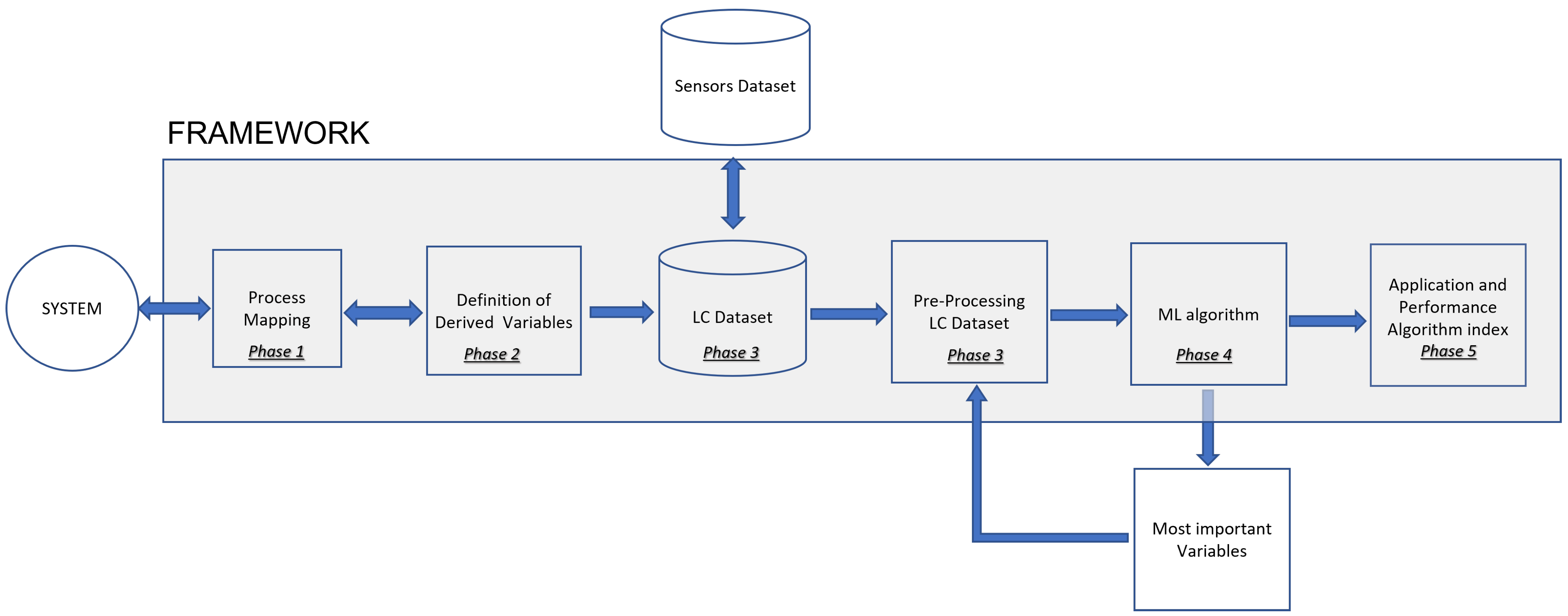
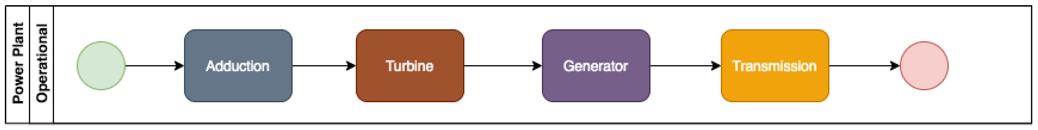
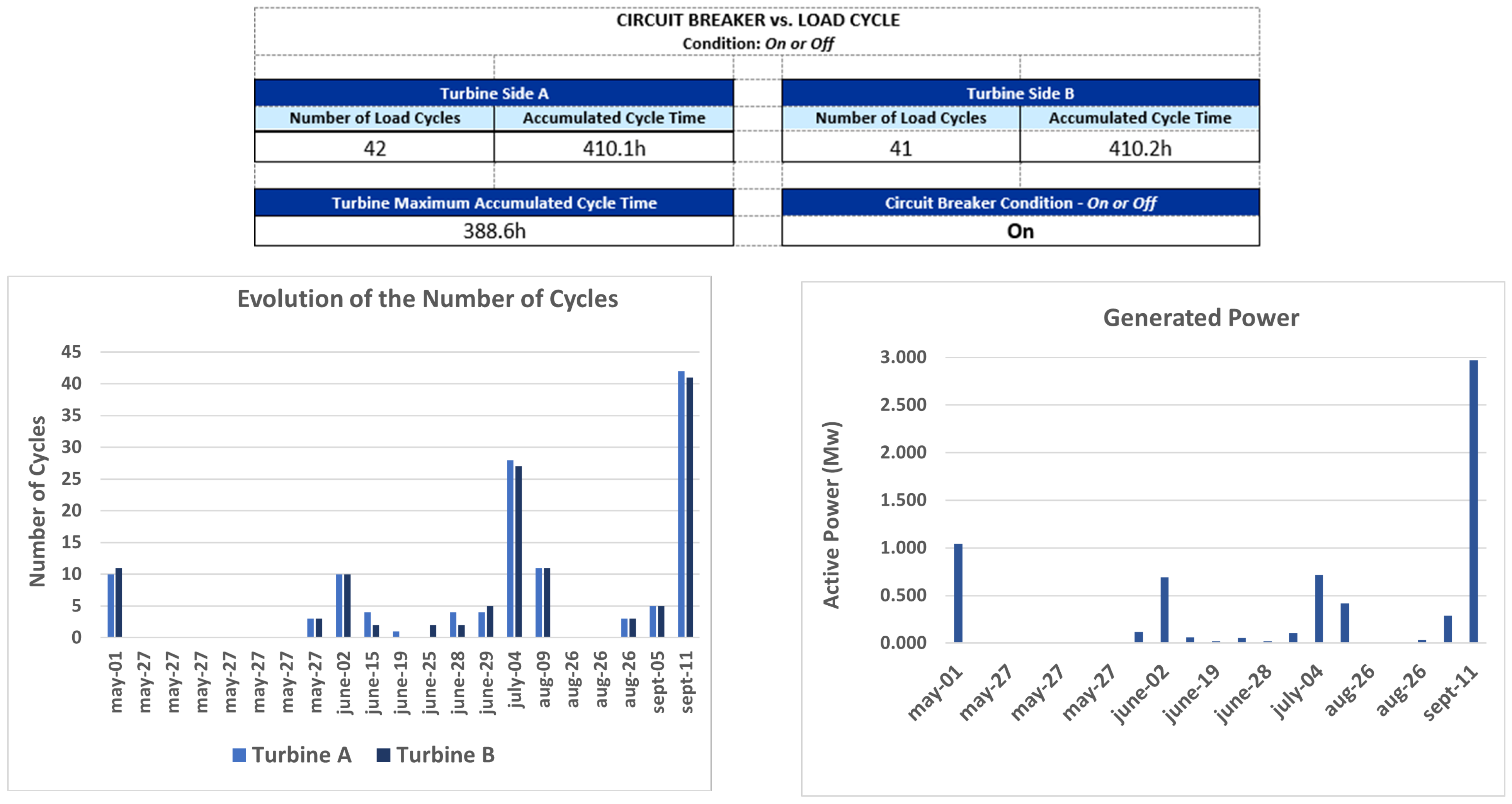
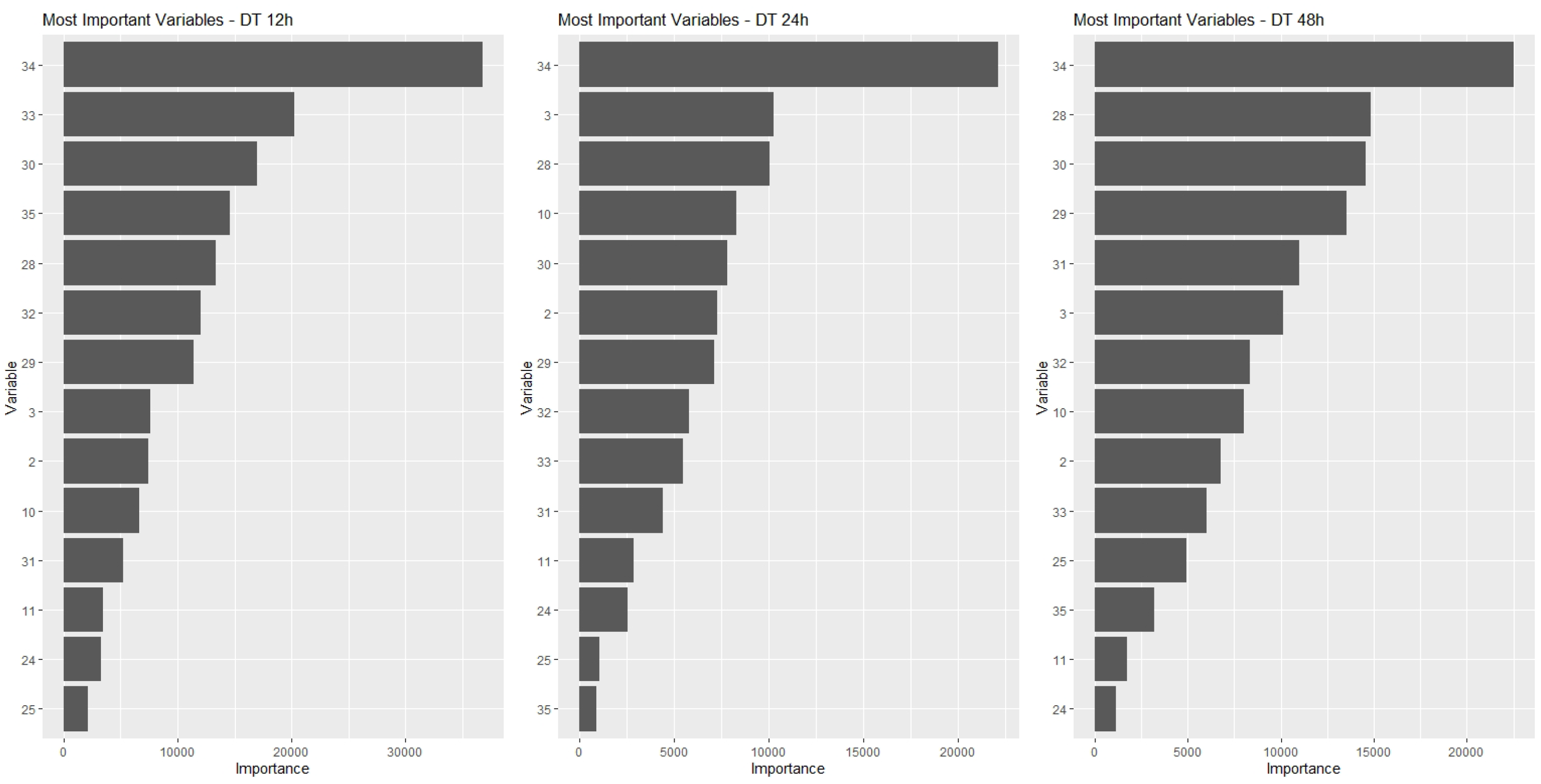
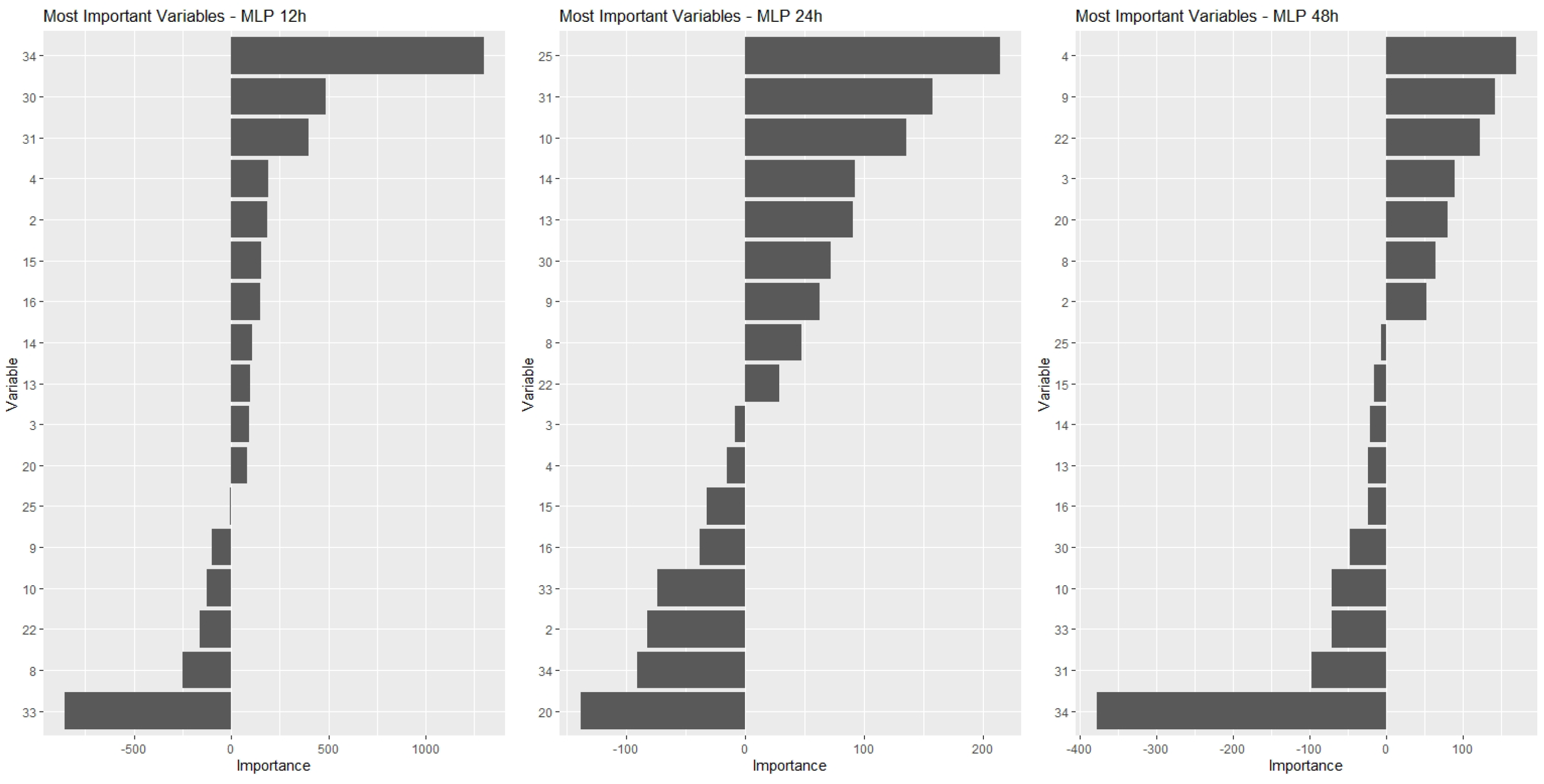
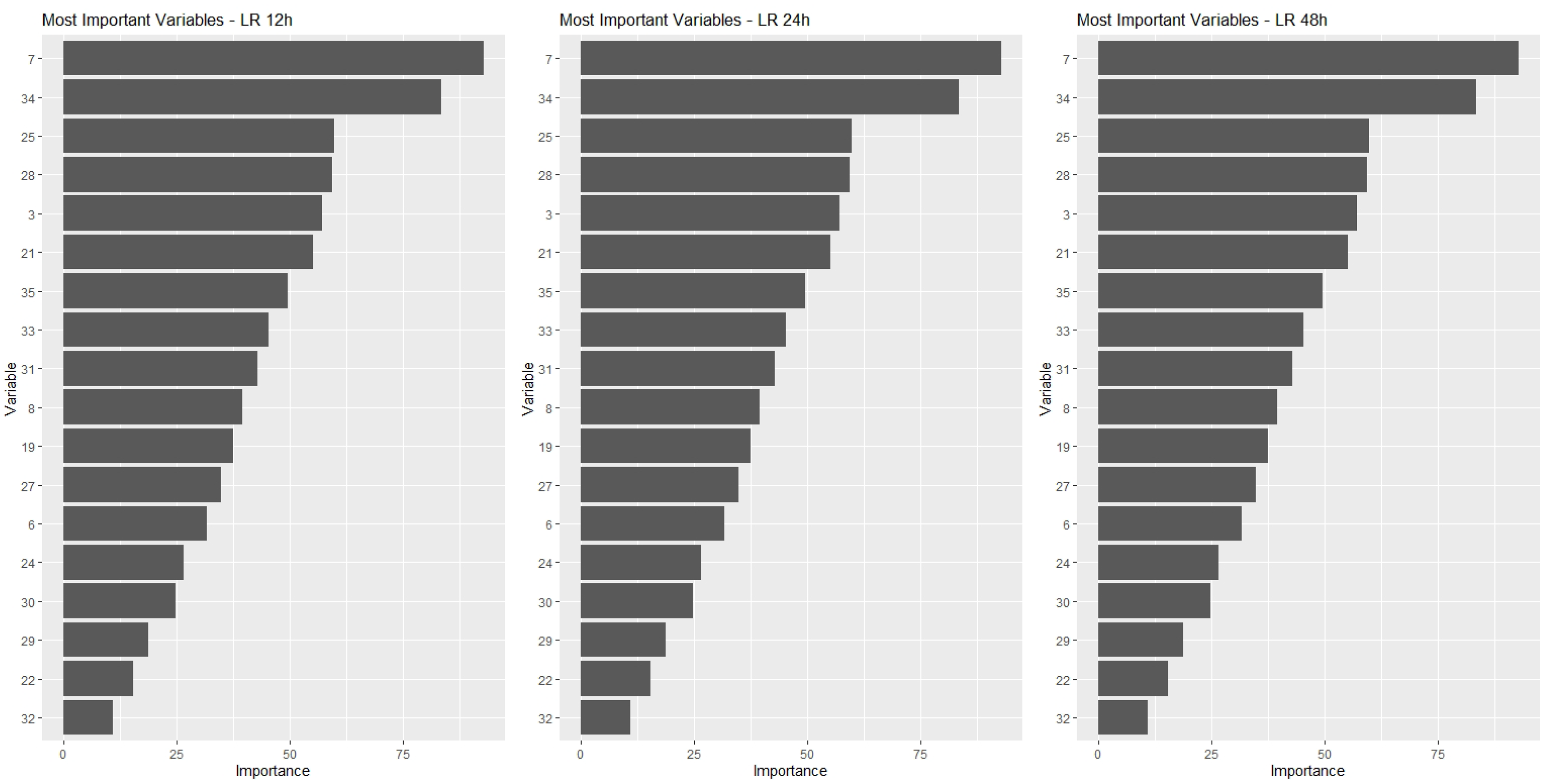
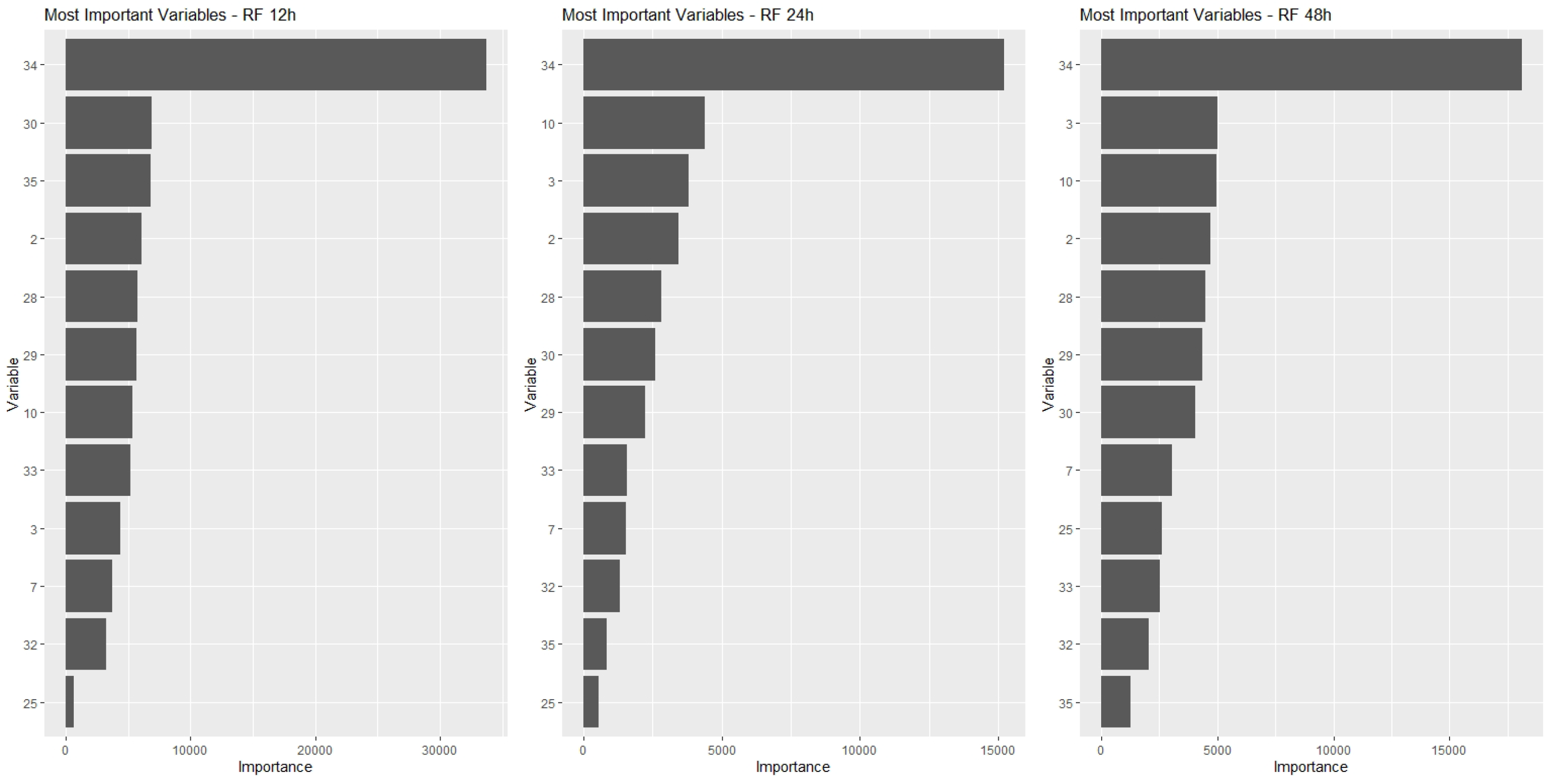
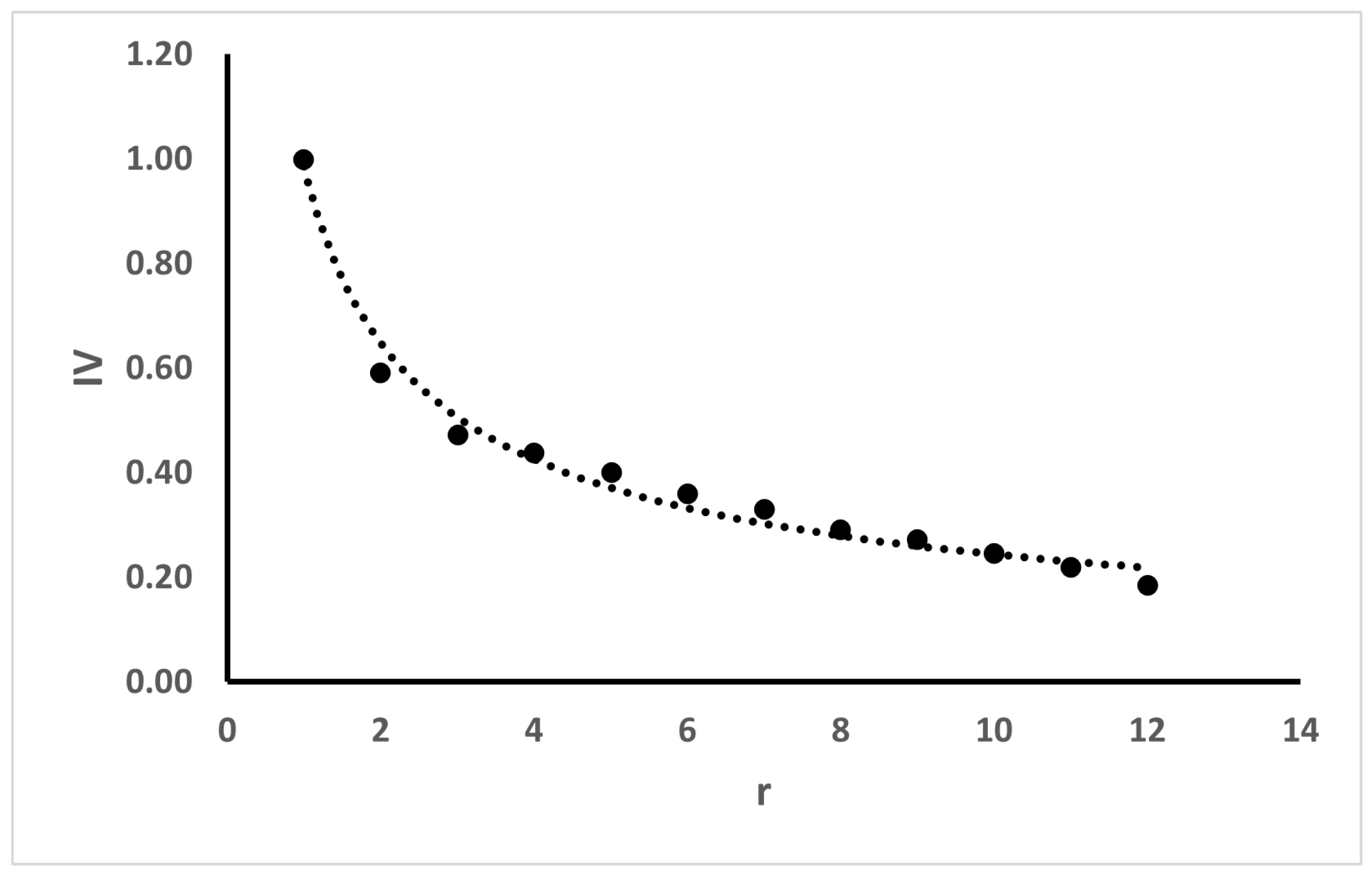
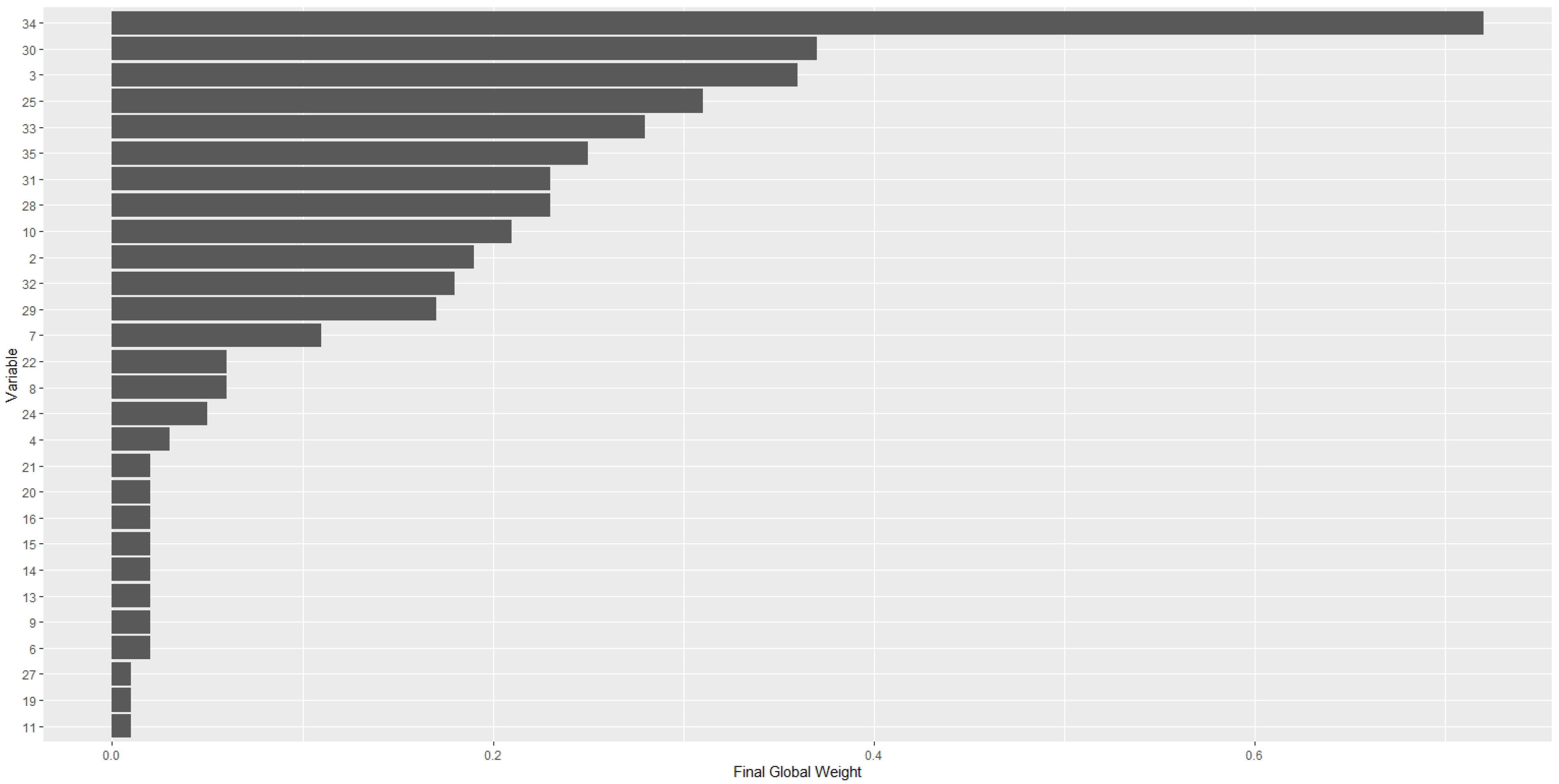
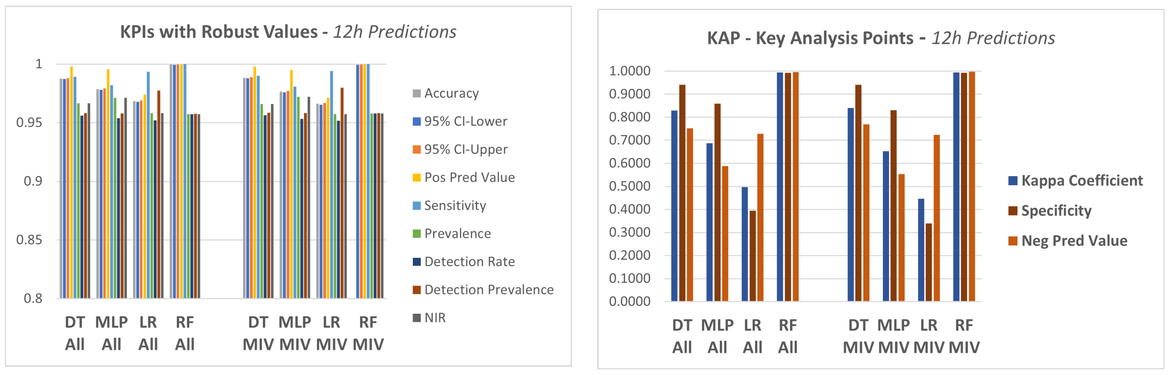
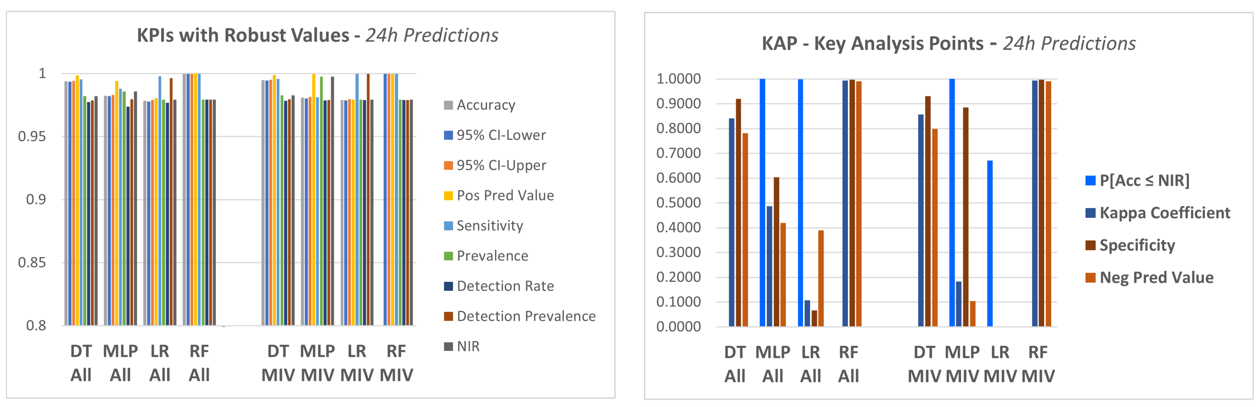
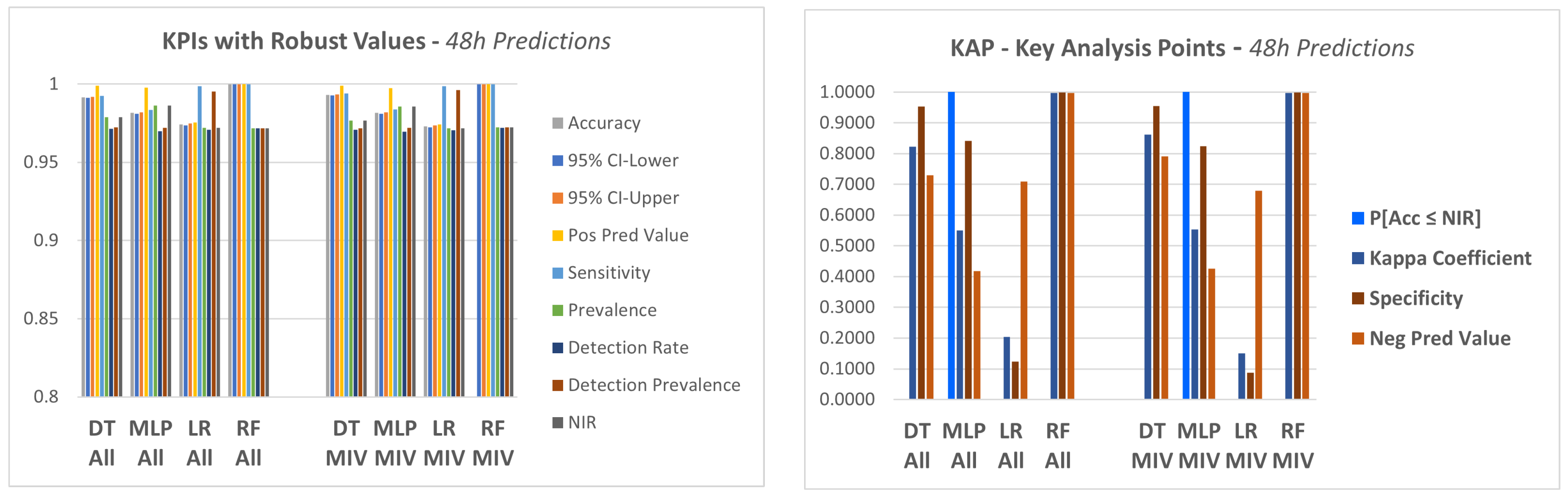
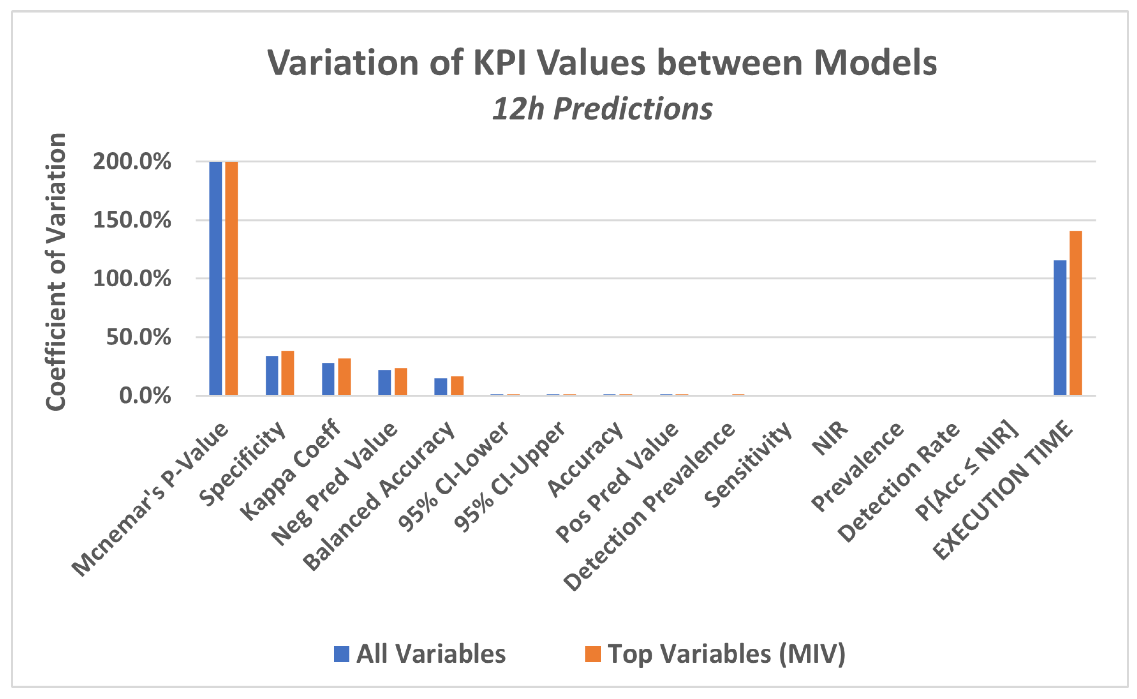
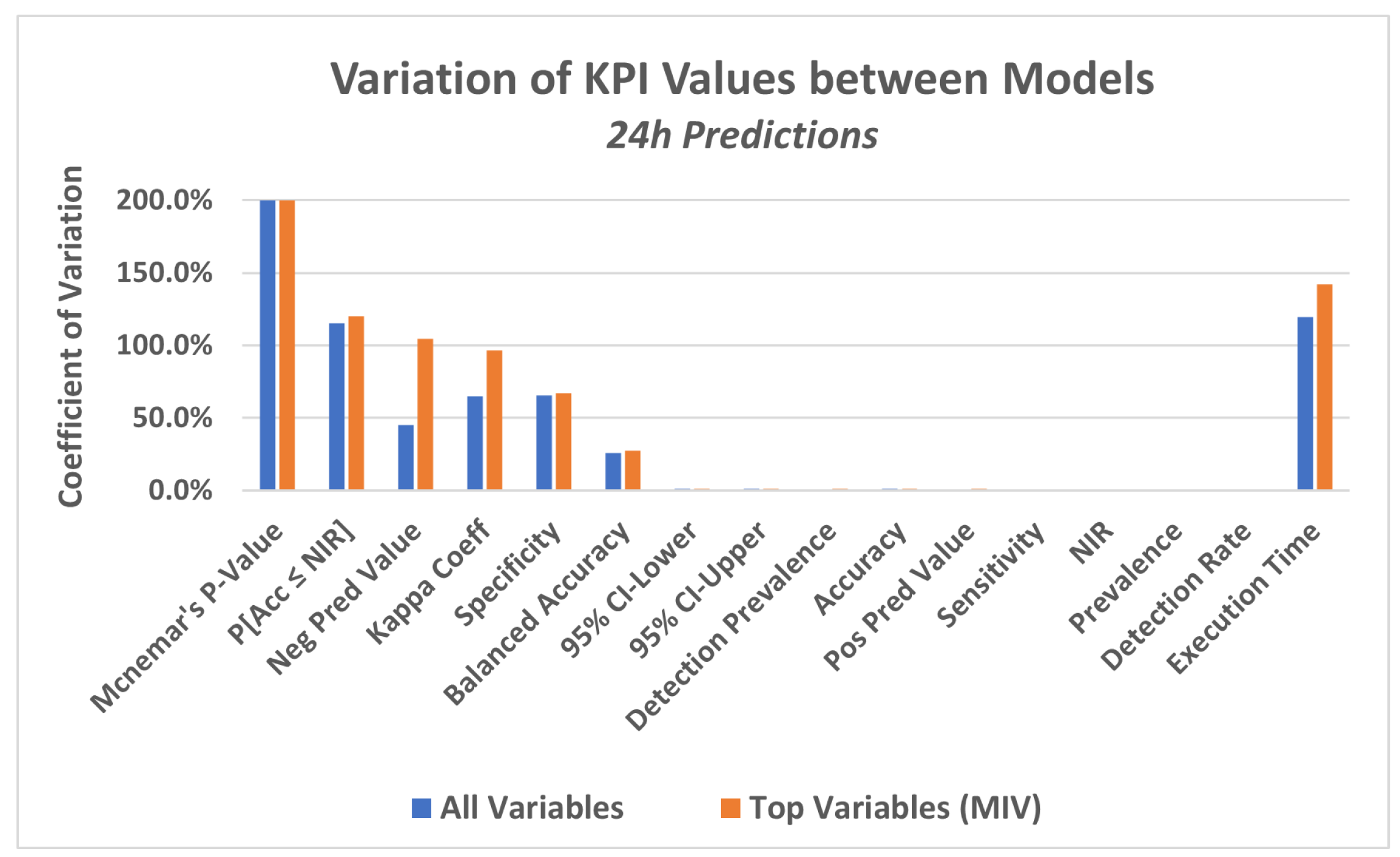
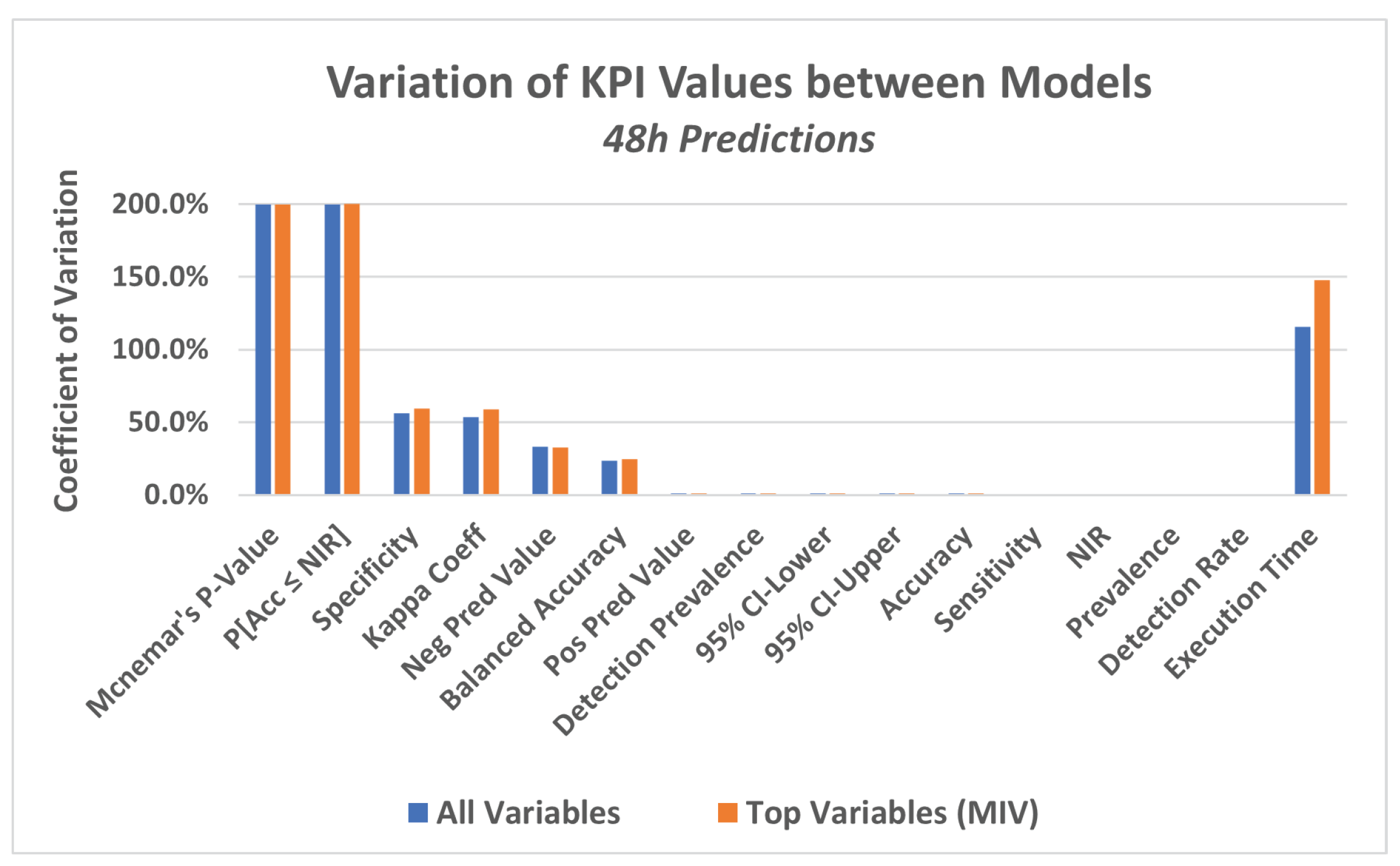
Publisher’s Note: MDPI stays neutral with regard to jurisdictional claims in published maps and institutional affiliations. |
© 2022 by the authors. Licensee MDPI, Basel, Switzerland. This article is an open access article distributed under the terms and conditions of the Creative Commons Attribution (CC BY) license (https://creativecommons.org/licenses/by/4.0/).