Article

Numerical Simulation Study on the Flow and Heat Transfer Characteristics of Subcooled N-Heptane Flow Boiling in a Vertical Pipe under External Radiation

Faculty of Metallurgical and Energy Engineering, Kunming University of Science and Technology, Kunming 650093, China
*
Author to whom correspondence should be addressed.
Energies 2022, 15(10), 3777; https://doi.org/10.3390/en15103777
Submission received: 30 March 2022 / Revised: 1 May 2022 / Accepted: 16 May 2022 / Published: 20 May 2022

Abstract

:
In the top submerged lance (TSL) smelting process, flow boiling may occur in the lance’s inner pipe due to the heat coming from the furnace when liquid fuel is adopted. In the current study, a numerical simulation was carried out by coupling the Eulerian two-fluid model with the improved RPI wall boiling model to investigate the subcooled n-heptane flow boiling in the inner pipe. The effects of inlet velocity and pipe wall emissivity on two-phase flow and heat transfer are elucidated. The results show that, for pipes with inlet velocity ranging from 0.3 m·s−1 to 1.0 m·s−1, an increase in inlet velocity leads to a lower void fraction near the outlet, as well as a lower average velocity and a lower average temperature of each phase. Meanwhile, the Onset of Nucleate Boiling (ONB) position approaches to the outlet, and the total pressure drop of the entire pipe reduces when the inlet velocity increases. However, the opposite trends appear when increasing the pipe wall emissivity. The maximum wall temperature corresponding to the critical heat flux (CHF) point is slightly affected by inlet velocity but significantly affected by pipe wall emissivity. The non-equilibrium effect and the specific components of pressure drop are also further investigated.

1. Introduction

The vertical lance is a critical component of the top submerged lance (TSL) process, which consists of a stainless-steel outer pipe and a carbon-steel inner pipe for injecting oxygen-enriched air and hydrocarbon fuel, respectively. The lance is vertically inserted into the furnace, surrounded by high-temperature off-gas and turbulent molten bath [1,2,3]. The outer pipe is continuously in a high-temperature state, and radiation is the dominant heat transfer mode between the inner pipe and the outer pipe. When liquid hydrocarbon fuel is adopted, flow boiling may occur within the inner pipe due to the external radiation from the outer pipe. Subcooled flow boiling is characterized by its large heat transfer coefficients. However, excessive-high heat flux on the wall may trigger the occurrence of boiling crisis, where the heat transfer coefficient deteriorates dramatically [4,5], and wall temperature increases rapidly. The occurrence of boiling changes the flow characteristics of the hydrocarbon fuel within the lance and affects the air-fuel mixture ejection from the lance tip. The pipe wall temperature rise caused by boiling crisis also accelerates lance wear. Moreover, since the lance generally has a length of several meters, once nucleate boiling occurs in the inner pipe, there may be a sufficient distance before the lance tip to develop boiling crisis.
The boiling crisis, where the surface is exposed directly to the vapor, is categorized into two types [6,7]. One is termed the departure from nucleate boiling (DNB), which occurs in low-quality region of film boiling, characterized by the high subcooling level. Additionally, the second type is dryout, which is triggered by depletion of the liquid film at high-quality flow conditions and typically in the annular flow. The maximum heat flux immediately before the boiling crisis is termed as the critical heat flux (CHF). In the vertical lance, the DNB-type boiling crisis is mostly expected to appear due to the high inlet subcooling of hydrocarbon fuel. Downstream of the CHF point, the two-phase flow enters post-CHF flow regimes. Resulting from the DNB mechanism, the post-CHF flow regimes includes inverted annular film boiling (IAFB), dispersed flow film boiling (DFFB) and the transition regime between them, i.e., inverted slug film boiling (ISFB).
Gas–liquid subcooled boiling flow is of enormous interest in many industrial applications such as the thermal engineering systems, electronic systems and nuclear reactors [8]. Numerous experimental studies have been conducted to determine the boiling mechanism of water and organic working fluid in various flow boiling regimes. Over the years, criteria for dividing the flow boiling regime are proposed [6,7,9], and empirical correlations are developed for specific operating conditions. A complete evaluation of the flow boiling phenomena and pressure drop of R134a in a smooth tube of 8.62 mm was presented by Celen et al.: they evaluated the effect of mass flux, saturation temperature and heat flux on the heat transfer coefficient, and how pressure drop was affected by mass fluxes for all conditions investigated [10]. Wang et al. investigated the impact of different factors on the flow boiling of R290 and R22 in double-concentric pipes. The results show that heat transfer coefficient, pressure drop, and exergy destruction are significantly impacted by the pipe diameter and the refrigerant velocity, but slightly impacted by water velocity and saturation temperature [11]. El Nakla et al. [12] conducted experiments to investigate IAFB of upward R-134a flow in a vertical pipe. Depending on the relation curve between heat transfer coefficient and quality, they divided the IAFB regime into four separate regions and discussed the different mechanisms of each. Based on the two-step model and took non-equilibrium effects into account, Shah [13] proposed a graphical predictive technique for film boiling heat transfer in vertical tubes at low reduced pressures. The correlation has been verified with experimental data for fluids, including water, hydrocarbons, and cryogens in a wide range of operational parameters, which includes thermodynamic equilibrium qualities from 0.1 to 2.9, diameters from 2.5 to 14.9 mm. In the subsequent research, the graphical predictive technique was developed into a general correlation by Shah and Siddiqui [14]. On those bases, the correlation has been further modified by Shah [15] to be applicable for heat transfer during DFFB in both vertical and horizontal tubes, and the new database included more points at reduced pressures greater than 0.8 and mini channels. IAFB and DFFB are the two basic types of flow film boiling. The void fraction in the IAFB regime is usually less than 0.5 or 0.6 [16,17], and in the DFFB regime is usually larger than 0.8 or 0.9, [18,19]. Additionally, the transition zone between these two regimes is known as ISFB regime [13,19]. Mohanta et al. [20] proposed a correlation for the Nusselt number during film boiling in a vertical channel of rod bundle based on a semi-empirical model. The correlation is developed using the experimental data with pressure ranging from 138 to 414 kPa, and applicable for void fraction up to 0.9, covering the IAFB and ISFB regime.
Xu and Fang [21] carried out a comparison among four leading two-phase frictional pressure drop correlations based on an experimental database in which most of the data have qualities between 0.2 and 0.8. They reported that correlations of Müller-Steinhagen and Heck [22] showed the best estimation. A new correlation was proposed by introducing the Laplace constant to the correlations of Müller-Steinhagen and Heck [22] to enhance the prediction performance in mini-channel. Xu et al. [23] have conducted a series of experiments on the flow boiling frictional pressure drop of saturated R134a at different conditions in the subsequent study, and the correlation is further evaluated. They indicated that frictional pressure drop increases with increasing mass flux and vapor quality; however, it decreases with increasing saturation pressure and hydraulic diameter. Yan et al. [18] experimentally investigated the pressure drop of highly subcooled water flow boiling in a vertical circular tube under high heat and mass fluxes. The parameter effects on subcooled boiling pressure drop show the same trends as Xu et al. [23] have reported. Additionally, they used the boiling number, Jacob number, and density ratio to predict the subcooled boiling pressure drop in their correlation proposed. Muszynski et al. [24] investigated the acceleration pressure drop component of R134a flow boiling in a horizontal tube, and evaluated the void fraction correlation for the acceleration pressure drop predictions under a variety of parameters conditions. They indicated that the void fraction correlation of Zivi [25] shows the best performance in acceleration pressure drop prediction, among other literature correlations. The data of acceleration pressure drop are acquired by comparing the two-phase frictional pressure gradients in the adiabatic and diabatic flow.
Performing boiling experiments under a specific condition are quite challenging due to the high-power requirements and difficulties in detection [26]. The applicability of established empirical correlations is limited to a specific range of operating parameters [5]. Therefore, the supplementation or even the replacements experiments by numerical simulations are of relevant interest. In conjunction with the Eulerian two-fluid model, the wall heat flux partition model has been validated to be an applicable approach [27,28]. Kurul [29] firstly proposed the wall heat flux partition model to predict the subcooled water flow boiling at a pressure of 4.5–5.0 MPa. The total heat flux from the wall to the liquid is divided into three components as the liquid phase convective heat flux, the quenching heat flux, and the evaporative heat flux. Additionally, he used the Eulerian two-fluid model as a framework for sub-models of heat, mass, and momentum transfer. The wall boiling model which decomposes the total wall heat flux into three components is now referred to as the basic Rensselaer Polytechnic Institute (RPI) model, and has been extended to a broader range of operating parameters. Tu et al. [30] extended the wall heat flux partition model to be applicable for low pressures of 0.11 to 0.17 MPa. They adapted the sub-models of mean bubble diameter and bubble departure diameter in Kurul’s model [29]. Zhang et al. [31] compared the performances of different turbulence models, wall functions, two-phase turbulence treatments in the subcooled flow boiling simulation. They reported that the results of k-ε models show better agreement with experimental data than k-w models, and the dispersed and per phase treatments for two-phase turbulence parameters performed no better than the mixture treatment when the void fraction is less than 0.5.
The basic RPI model assumes that the gas phase temperature is fixed at the saturation temperature, and performs well in predicting nucleate boiling regime [32,33,34]. However, the basic RPI model’s accuracy is reduced in modeling the DNB regime, or up to the Critical Heat Flux (CHF) and post-CHF regime, where the vapor phase is in contact with the heated surface periodically or continuously [5,35]. Lavieville et al. [36] repartitioned the wall heat flux of the basic RPI model, included the vapor temperature in the simulation procedure. The basic RPI model has been extended for modeling the downstream of the DNB regimes, which is known as the improved RPI model. Zhang et al. [37] employed the improved RPI model to investigate the DNB phenomena in vertical pipes under an extremely high heat flux of about 50 MW·m−2. The predicted results agreed quite well with the experimental data of Celata et al. [38], and the deviations are less than 15.0%. Li et al. [39] used the improved RPI model to simulate the DNB regime in both uniform and non-uniform heated vertical tubes under high pressures. The sensitivity of the critical void fraction αdry was discussed. They concluded that a modification in the critical void fraction could make the prediction better. Maytorena and Hinojosa [40] modeled the subcooled flow boiling in the vertical circular tubes of an external solar tower receiver based on the improved RPI model. Non-uniform heat flux is applied on the tube, and the working fluid is at a pressure of 4.5 MPa. The results show that the CFD approach satisfactorily reproduces experimental data.
Although a considerable number of numerical studies on the flow boiling of organic working fluids have been reported, most of them are cryogenic fluids or refrigerants [41,42,43], numerical studies for hydrocarbons with higher saturation temperature have barely appeared. The hydrocarbon fuel flows vertically downwards in a TSL lance; however, the investigations on flow boiling of the vertically downward flow are rather rare [44]. Generally, the liquid fuel added through the lance is fossil fuel or biomass fuel [1,2]. Considering fluctuations exist in the properties of fossil fuel and biomass fuel, in this study, the n-heptane has been chosen as the working fluid for its similar thermal and transport properties as diesel and gasoline. The physical properties of n-heptane are from the literature [45,46].

2. Numerical Methodology

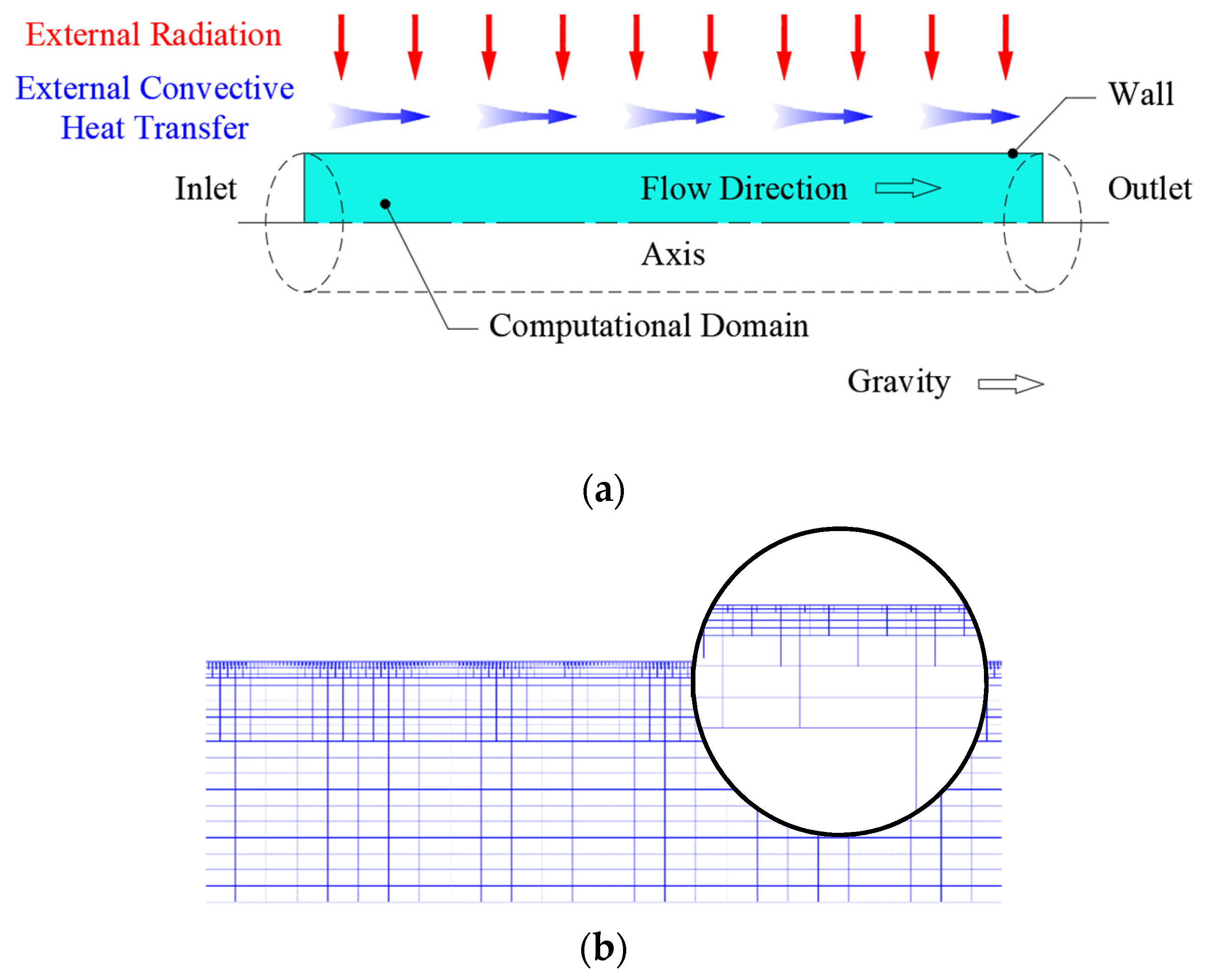
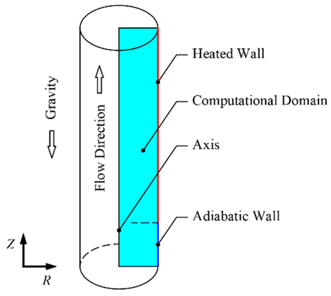
2.1. Definition of the Physical Problem

The geometry model is established based on the actual dimensions of a typical TSL furnace [47]. Detailed parameters of the furnace are listed in Table 1. Figure 1 shows the schematic of the TSL lance. The outer pipe cross-section is annular, and the inner pipe cross-section is circular, so the entire lance has a strict axisymmetric structure.
The outer pipe is directly in contact with the off-gas and molten bath and continuously in a high-temperature state. The heat from the outer pipe is transferred to the inner tube by radiation. The flow rate of the oxygen-enriched air in the annular channel of the outer pipe is high enough that the oxygen-enriched air in the area away from the heating wall is barely heated through the convention, even if it runs through the entire channel. Moreover, nitrogen and oxygen are generally considered as a transparent medium because they absorb or emit only a very insignificant amount of radiation. The oxygen-enriched air cannot be heated by radiation either. Consequently, the oxygen-enriched air is continuously cooling the inner and outer pipe walls. For the inner pipe, the heat taken away by convection accounts for about 10% of the incoming heat from radiation. Therefore, the radiative heat transfer from the outer pipe to the inner pipe and the convective heat transfer between the oxygen-enriched air and the inner tube wall can be simplified to a one-dimensional boundary condition on the inner pipe wall.
The schematic diagram of the computational domain is illustrated in Figure 2a. The diameter of the inner pipe is 15 mm, and the length is 5.5 m. A half-section of the pipe was modeled in the cylindrical coordinate and discretized using a structured rectangular grid, as shown in Figure 2b. The grid cells are refined in the near-wall area, the maximum cell size is 0.5 mm × 1.0 mm, and the minimum size is 31.25 μm × 62.5 μm. The total number of elements in the computational domain is 720,552.
The present work was conducted for different inlet velocity and pipe wall emissivity conditions. As listed in Table 2, two series of cases were proposed, namely the different inlet velocities under the same pipe wall emissivity condition and the different pipe wall emissivity with the same inlet velocity. The flow rate of the n-heptane at the inlet was taken as the mass flow rate, with a value ranging from 204.15 kg·m−2·s−1 to 680.5 kg·m−2·s−1 (converted into the average velocity is 0.3 m·s−1 to 1.0 m·s−1 at the initial temperature). The pressure outlet boundary condition was used for the inner pipe tip. The inner pipe wall emissivity was set from 0.4 to 0.8, and the outer pipe was regarded as the external radiation source with a temperature of 1400 K. The external convection heat transfer caused by oxygen-enriched air was calculated in a simplified manner by using an exterior heat transfer coefficient of 50 W·m−2·K−1 and an average oxygen-enriched air temperature of 293.15 K. Both the external radiative and convective heat transfer are adopted to the one-dimensional non-slip boundary condition on the wall.

2.2. Modeling Assumptions

In order to establish a reasonable and simplified simulation model, the following assumptions are adopted:
(1)
The mass flow rate is steady.
(2)
The outer pipe temperature is steady and consistent with the temperature of the off-gas in the furnace.
(3)
The inner and outer tube walls are regarded as diffuse surfaces.
(4)
The inner pipe is entirely covered by the outer pipe, ignoring the influences of unclosed surfaces at the inlet and outlet. That is, the view factor of radiation between the outer pipe and the inner pipe takes a value of 1.
(5)
Since the convective heat transfer caused by the oxygen-enriched air has a limited effect on the overall heating condition of the wall, and the convective heat transfer coefficient changes slightly with the wall temperature, the fluctuations in the convection heat transfer coefficient are ignored.
(6)
The oxygen-enriched air in the annular channel is optically transparent.
(7)
The average temperature of the oxygen-enriched air in the annular channel is at a fixed value.
(8)
The inner pipe wall thickness and thermal resistance are ignored.

2.3. Governing Equations

2.3.1. Wall Boundary Condition

This work focuses on the flow boiling characteristics in the inner pipe, not aimed at the heat transfer process of oxygen-enriched air inside the outer pipe. Therefore, the external radiative and convective heat transfer were modeled by the one-dimensional thermal boundary condition on the wall. This treatment reduces the computational costs without compromising the accuracy of the solutions.
Based on the assumption, the heat transferred from the outer pipe by radiation qra can be expressed as:
q ra = ε ext σ ( T O 4 T I 4 )
ε ext = 1 1 ε I + A I A O ( 1 ε O 1 )
where εext is the equivalent emissivity, σ is the Stefan-Boltzmann constant, TO is the temperature of the outer pipe wall, TI is the temperature of the inner pipe wall, εO is the emissivity of the outer pipe wall, εI is the emissivity of the inner pipe wall, AO is the side surface area of the outer pipe, AI is side the surface area of the inner pipe.
The exterior convective heat transfer caused by oxygen-enriched air outside the inner pipe can be expressed as:
q co = h ext ( T air T I )
where hext is the heat transfer coefficient between the oxygen-enriched air and the pipe wall, Tair is the average temperature of oxygen-enriched air.
Finally, the thermal boundary conditions on the inner pipe wall are defined as:
q w = q ra + q co = ε ext σ ( T I 4 T O 4 ) + h ext ( T air T I )

2.3.2. Eulerian Two-Fluid Model

Since the fluid temperature varies significantly in the entire computational domain, the variations in physical properties of each phase with temperature were taken into account. For the liquid phase, it was assumed that its properties are only related to temperature, effects of pressure were ignored; a reference pressure of 1 atm was adopted instead. Data on the liquid n-heptane properties, at a temperature range from 293 K to 400 K and pressure of 1 atm, are from the literature [45,46]; linear interpolation is adopted to estimate the value between data points. For the vapor phase, it was regarded as an ideal gas when dealing with the thermodynamic properties of density and specific heat. Additionally, the transport properties of vapor phase, including viscosity and thermal conductivity, were taken from the values of vapor n-heptane at a temperature range from 371 K to 600 K and pressure of 1 atm. The vapor n-heptane properties are also from the literature [45,46]. Moreover, the saturation temperature was set to change with static pressure.
In the Eulerian two-fluid model, each phase is considered as a continuous phase. Additionally, the continuity, momentum, and energy equation for each phase were solved separately. Here, the subscript i represents either the vapor or liquid phase, and the subscript j is the non-i phase.
Continuity equation for phase i:
t ( α i ρ i ) + ( α i ρ i v i ) = ( m ˙ ji m ˙ ij ) + S M , i
where α is the volume fraction, ρ is the density, v is the velocity, m ˙ ji is the mass transfer from the j phase to i phase, and m ˙ ij is the mass transfer from the i to j phases, SM is the mass source term.
Momentum equation for phase i:
t ( α i ρ i v i ) + ( α i ρ i v i v i ) = α i p + τ i = + α i ρ i g + ( m ˙ ji v ji m ˙ ij v ij ) + F INT , i
where p is the static pressure, τ = is the stress–strain tensor, vji and vij are the interphase velocity, and FINT is the interfacial momentum transfer between the two phases, which includes drag force, lift force, wall lubrication force, turbulent dispersion force and virtual mass shown as follows:
F INT , i = F D , i + F L , i + F WL , i + F TD , i + F VM , i
Stress tensor and strain tensor was introduced as τ = in the momentum equation, due to the nonconstant density of each phase. For phase i, the stress–strain tensor can be expressed as:
τ = i = α i μ i ( v i + v i T ) α i ( p + 2 3 μ i v i ) I =
where I = is the unit tensor.
Energy equation for phase i:
t ( α i ρ i h i ) + ( α i ρ i v i h i ) = α i d p i d t q i + S E , i + Q ij + ( m ˙ ji h j m ˙ ij h i )
where h is the specific enthalpy, q is the heat flux, SE is the energy source term, Qij is the intensity of heat exchange between the two phases.

2.3.3. Improved RPI Model

For the basic RPI model, the wall heat flux is partitioned into three components: the liquid phase convective heat flux qC, the quenching heat flux qQ, and the evaporative heat flux qE [42].
q w = q C + q Q + q E
However, considering the direct contact between the vapor phase and the wall, an extra heat flux qv is taken into account in the improved RPI model, which represents the convective heat flux of the vapor phase [36]. The wall heat flux partition is modified as:
q W = ( q C + q Q + q E ) f ( α L ) + [ 1 f ( α L ) ] q V
where αL is the liquid phase volume faction, f(αL) is a function of αL adopting the definition of Lavieville et al. [36], and can be expressed as:
f ( α L ) = { 1 0.5 exp [ 20 ( α L α crit ) ] α L α crit 0.5 ( α L α crit ) 20 α crit α L < α crit
where the value of αcrit is 0.2, and the graph of f(αL) vs. αL has been plotted by Mali et al. [37] in their numerical study.
The liquid phase convective heat flux is defined as:
q C = h C ( T w T l ) ( 1 A b )
where hC is the liquid phase heat transfer coefficient, Tw is the wall temperature, Tl is the liquid temperature. The area of the heated wall is divided into two parts, Ab is the area covered with nucleating bubbles which is also known as the area of influence; thus, (1 − Ab) refers to the area covered with liquid.
A b = min ( 1 , K N w π D w 2 4 )
where K is an empirical constant based on the research of Del Valle and Kenning, and is calculated by
K = 4.8 exp ( J a sub 80 )
Jasub is the subcooled Jacob number
J a sub = ρ L C pL ( T sat T L ) ρ V h LV
where CpL is the specific heat of liquid phase, Tast is the saturation temperature, TL is the liquid phase temperature, ρv is density of the vapor phase, hLV is the latent heat of evaporation.
Nw is the nucleate site density given by Lemmert and Chawla model, and Dw is the departure diameter of bubbles given by Tolubinsky and Kostanchuk model.
N w = 210 1.805 ( T w T sat ) 1.805
D w = min [ 0.0014 , 0.0006 exp ( T w T sat 45.0 ) ]
The quenching heat flux models a portion of the heat from wall due to liquid filling the wall vicinity after bubble detachment, and is given by:
q Q = 2 k l π λ l τ ( T w T l )
where kl is the thermal conductivity of the liquid phase, λl is the thermal diffusivity defined as equation. τ is the periodic time and equal to the reciprocal of the bubble departure frequency f.
λ L = k L ρ L C pL
f = 1 τ = 4 g ( ρ L ρ V ) 3 ρ L D w
The evaporative heat flux is defined as the latent heat carried away by the detached bubbles. Assuming the bubbles are spherical, the evaporative heat flux can be calculated by
q E = N w ρ V h LV f π D w 3 6
The vapor phase convective heat flux is defined as:
q V = h V ( T w T v )
where hV is the vapor phase heat transfer coefficient.

2.4. Model Settings

In the current study, the flow regime includes all stages from subcooled flow boiling to DNB, and even DFFB occurs in some cases; therefore, the transition of the liquid phase from a continuous phase to a discrete phase needs to be considered in the model setup. The specific model settings are shown in Table 3.

2.5. Parameter Definition

The homogenous model treats the vapor and liquid phases as a homogeneous mixture flowing with the same velocity. From this definition, the homogenous model void fraction is the volume fraction of the vapor phase [48]. The cross-section averaged void fraction in the homogenous model can be expressed as:
α = A v A v + A l
where Av and Al are the areas covered with vapor and liquid, respectively.
Two quality models are involved in this work, namely the homogenous model quality and the thermodynamic equilibrium quality. Both of the two models are important parameters for describing the boiling state in flow boiling, and the distinction between these models is significant [49]. The homogenous model quality xho and the thermodynamic equilibrium quality xeq are defined as [33,49]:
x ho = α ρ v α ρ v + ( 1 α ) ρ l
x eq = h f h l h lv
where hf is the specific enthalpy of the vapor-liquid flow, hl is the specific enthalpy of the saturated liquid phase, and hlv is the vaporization latent heat.
The heat transfer coefficients are evaluated based on the difference between the inside wall temperature Tw and the saturation temperature Tsat corresponding to the local static pressure.
h = q T w T sat
For flow boiling in a circular pipe, the total pressure drop is due to the variation in kinetic and potential energy, and also due to friction at the wall. The total pressure drop ptot can be divided into three components of acceleration pressure drop, gravitational pressure drop, and frictional pressure drop, which is shown as:
Δ p tot = Δ p fri + Δ p grav + Δ p acc
The gravitational term is defined as [9,50]:
Δ p gra = 0 Z [ α ρ v + ( 1 α ) ρ l ] g sin θ d Z
where θ is the inclination angle of the pipe. For vertical downward flow, the inclination angle is −90°. Thus, the gravitational pressure drop can be expressed as:
Δ p gra = 0 Z [ α ρ v + ( 1 α ) ρ l ] d Z
The variations in velocity cause the acceleration pressure drop. For the straight pipe with a uniform diameter, the acceleration term can be expressed by:
Δ p acc = G 2 { [ ( 1 x ) 2 ρ l ( 1 ε ) + x 2 ρ v ε ] out [ ( 1 x ) 2 ρ l ( 1 ε ) + x 2 ρ v ε ] in }
where G is the mass flux, ε is a slip ratio model void fraction. Since it has been reported that the acceleration pressure drop could be overestimated when using the homogeneous model void fraction [23,51]. In this work, Zivi’s correlation [19] is adopted, which is a widely used slip ratio correlation for acceleration pressure drop prediction based on the minimum entropy production principle [48]. It is defined as:
ε = [ 1 + ( 1 x x ) ( ρ v ρ l ) 2 3 ] 1
Since the total pressure drop is obtained from the static pressure, the frictional pressure drop is calculated as:
Δ p fri = Δ p tot ( Δ p grav + Δ p acc )

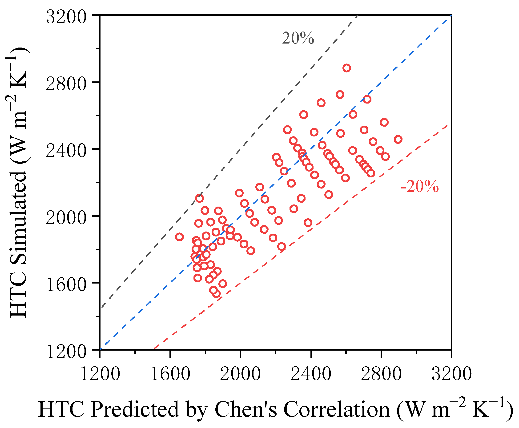
2.6. Model Validation

At present, most of the numerical studies on the flow boiling of organic media are carried out for low-temperature fluids or refrigerants. There are few studies on the flow boiling of hydrocarbons with high saturation temperature at atmospheric pressure, and the research on the vertically downward flow boiling is rare. This makes it difficult to obtain the relevant data of flow boiling in the vertical lance through experiments, nor can it be calculated through empirical formulas. Therefore, in this section, the model in this paper is applied to simulate the saturated flow boiling of n-heptane in a circular tube, and the simulation results are compared with the prediction results of the correlation of Chen [52] to verify the validity of the model.
The geometric model used in this section is shown in Figure 3, with a diameter of 15 mm, a total pipe length of 0.8 m and a heating section length of 0.75 m. The grid division is shown in Figure 4. The total number of elements in the computational domain is 112,000, the maximum cell size is 0.4 mm × 0.25 mm, and the minimum cell size is 0.1 mm × 0.25 mm.
The simulation conditions of saturated flow boiling of n-heptane simulated in this section are shown in Table 4. The inlet subcooling temperature of n-heptane was 0.5 K and the ambient pressure was 1 atm. The inlet velocity of 0.2~0.6 m·s−1 was calculated when the wall heat flux density of 10 kW·m−2. Additionally, the wall heat flux density of 12~26 kW·m−2 for an inlet velocity of 0.6 m·s−1 was calculated.
Figure 5 shows the distribution of void fraction and liquid phase velocity around the cross-section where the average void fraction is 0.5 when wall heat flux density is 10 kW·m−2. The figure shows the calculation area with the pipe axis on the left and the heated wall on the right, with the z-axis scale in m.
The Chen [52] correlation verified the heat transfer coefficient, which is based on saturated boiling experiments with water, methanol, n-heptane, cyclohexane, n-pentane and benzene in a macroscopic vertical circular tube. The Chen [52] correlation as follows:
h t p = S h n b + F h s p , l
h n b = 0.00122 k l 0.79 C p , l 0.45 ρ l 0.49 ( T w T sat ) 0.24 [ P s a t ( T w ) P l ] 0.75 σ 0.5 μ l 0.29 h f g 0.24 ρ g 0.24
h s p , l = 0.023 Re l 0.8 Pr l 0.4 ( k l D i )
where hnb is the heat transfer coefficient due to nucleation boiling, hsp,l is the heat transfer coefficient due to single-phase convection, S is the microscopic heat transfer suppression coefficient, F is the turbulence enhancement factor, kl is the thermal conductivity of the liquid phase, Cp,l is the specific heat capacity of the liquid phase, ρl is the density of the liquid phase, σ is the surface tension between the gas and liquid phases, μl is the viscosity of the liquid phase, hfg is the latent heat of vaporization and ρg is the density of the liquid phase.
Figure 6 shows the heat transfer coefficient comparisons between simulation results and Chen’s correlation, the equidistant points are the void fraction of 0.4~0.65 near the wall of the pipeline section, the bule line is the results of Chen’s correlation, the black and red lines are the 20% deviation of Chen’s correlation. As can be seen from the graph, all equidistant points are within a 20% deviation. This shows that the model in this paper can predict the saturated flow boiling of n-heptane in a vertical tube very well, and also has good predictive reliability for the subcooled boiling studied in this paper.

3. Results and Discussion

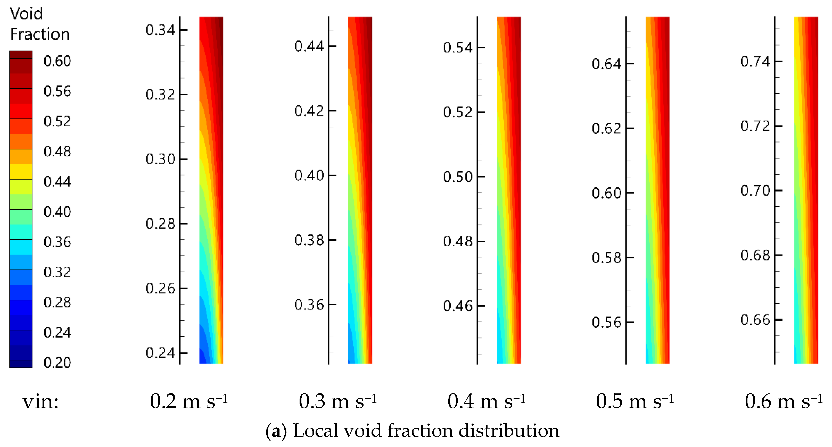
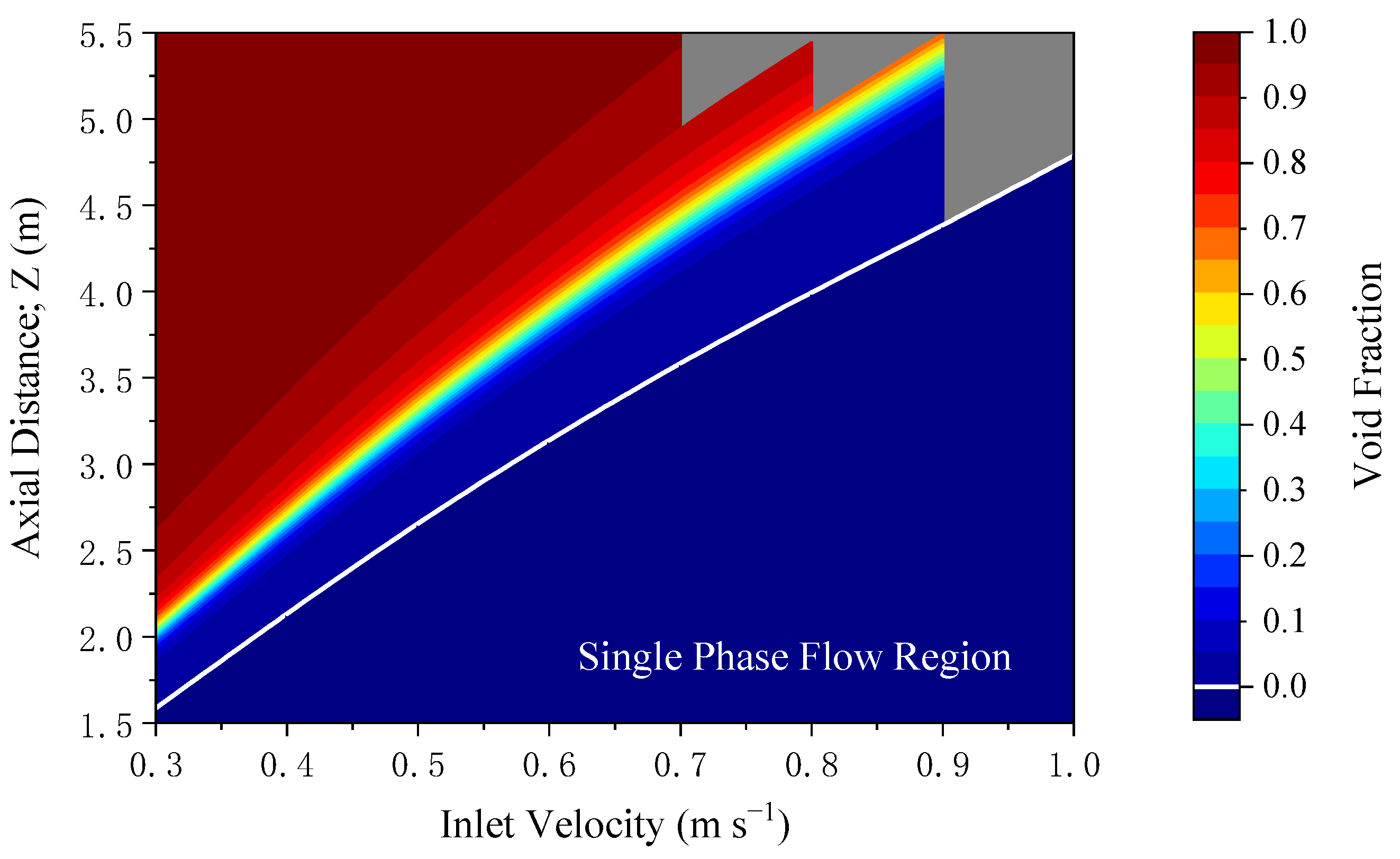
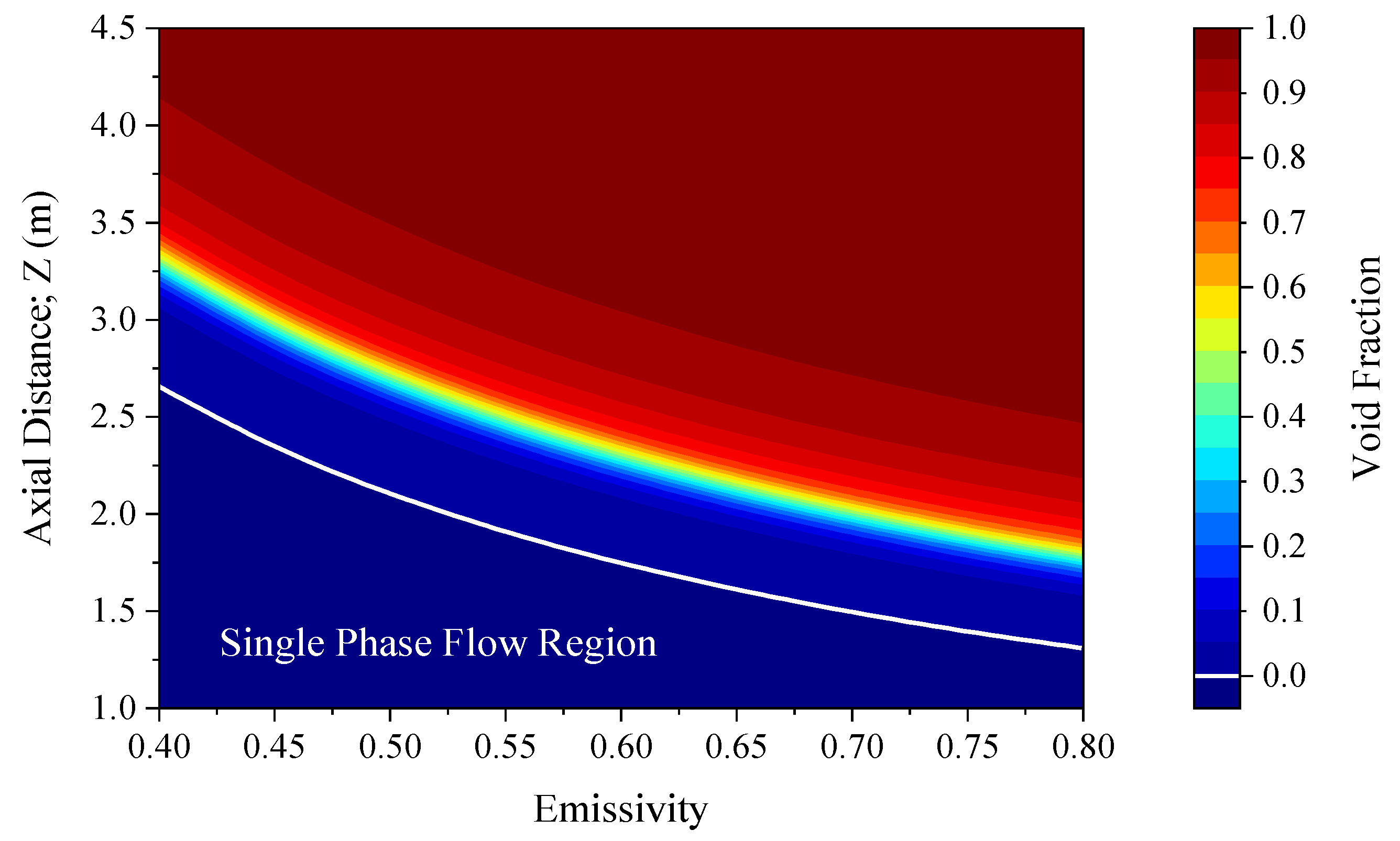
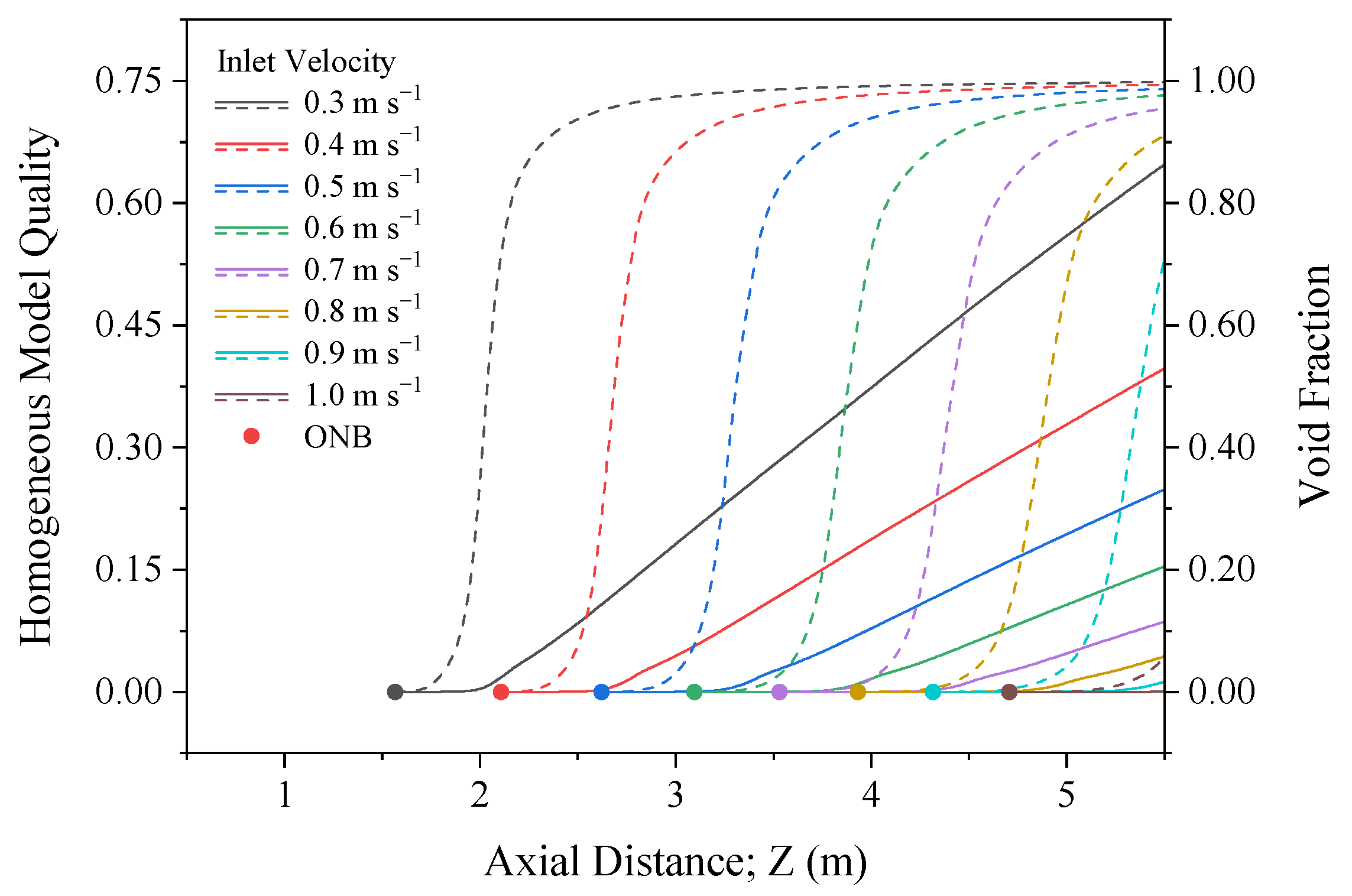
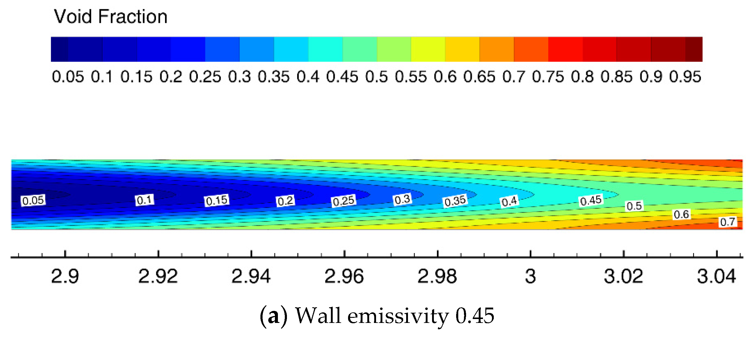
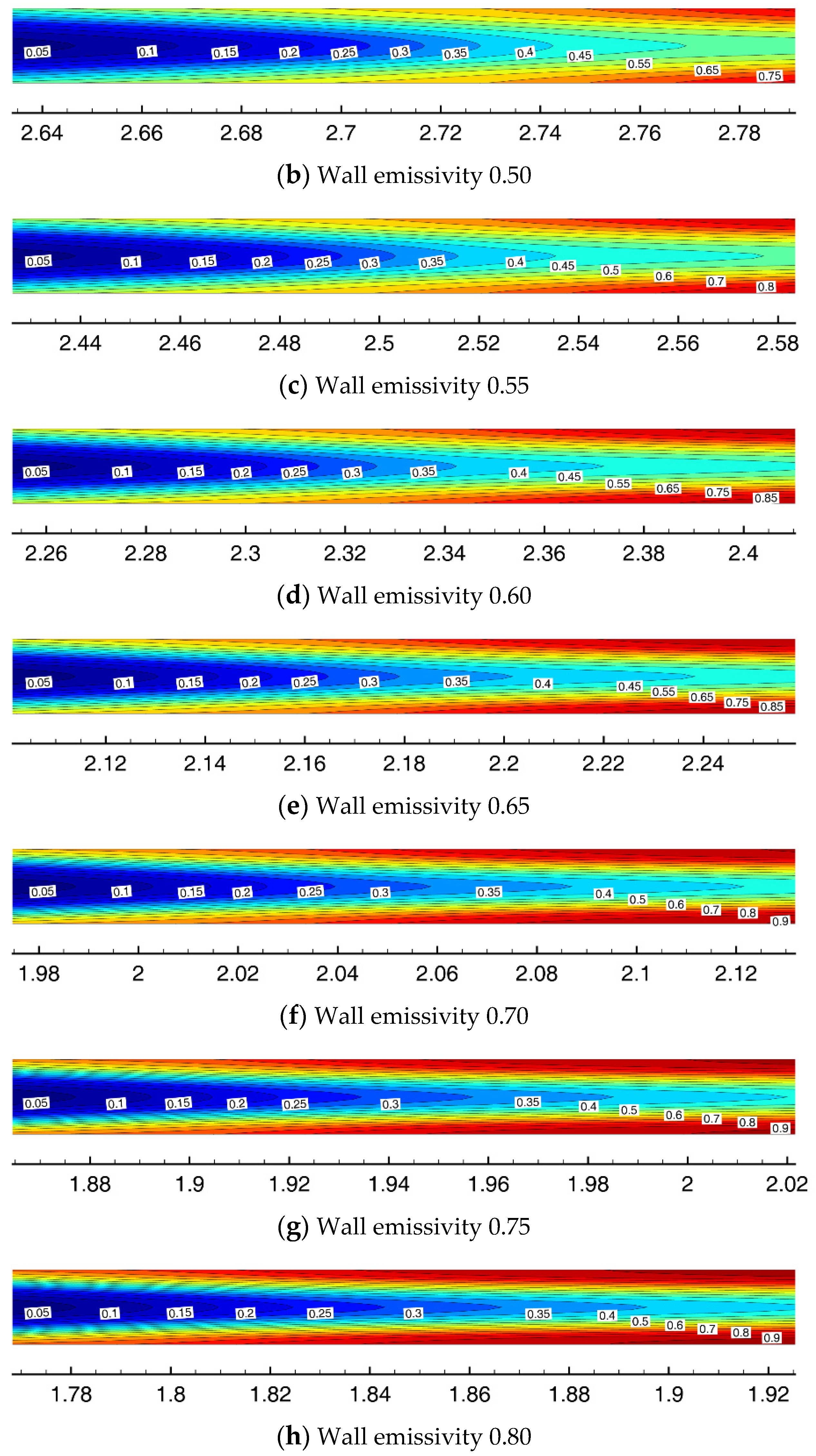
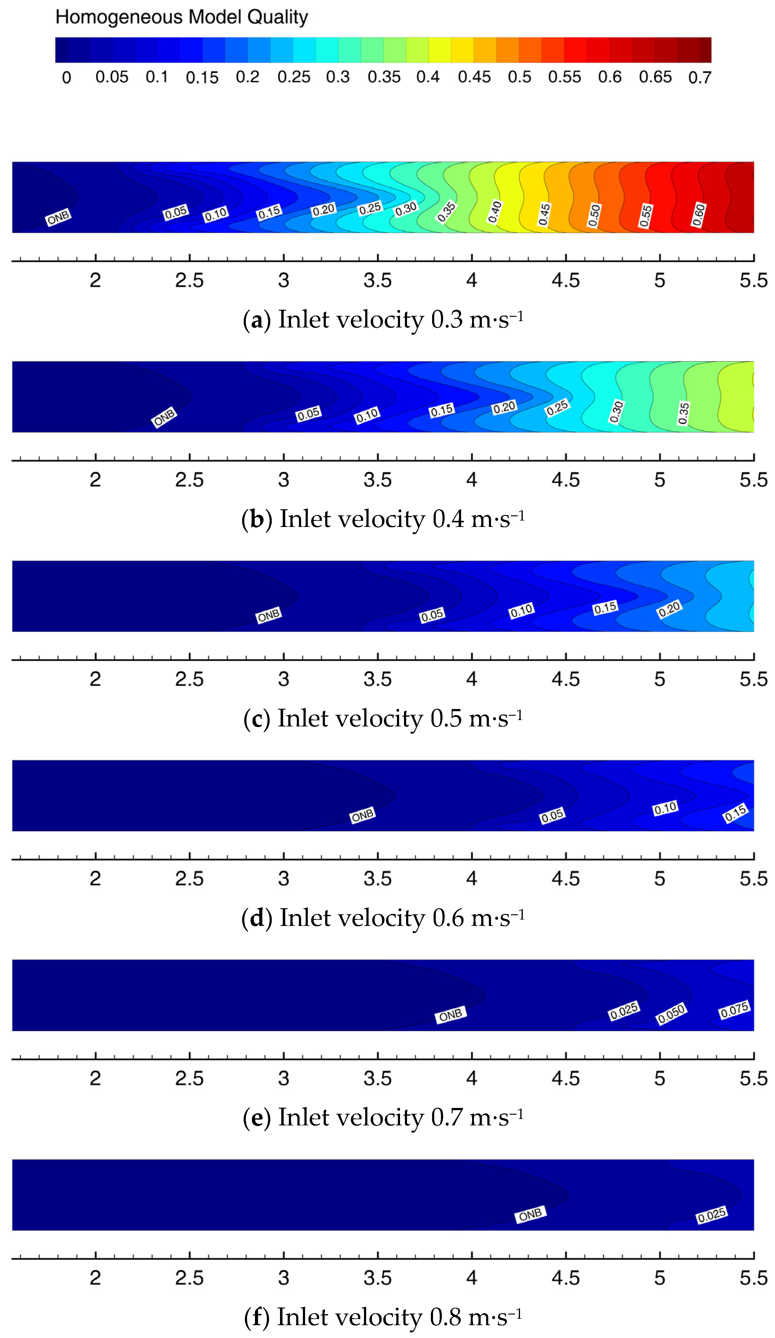
3.1. Void Fraction and Quality

Figure 7 shows the void fraction profiles along the axial direction of cases with different inlet velocity and Figure 8 shows that of cases with different pipe wall emissivity, which are listed in Table 2. The average void fraction of a specific cross-section can be quickly obtained from Figure 7 and Figure 8 as long as the operating condition matches. The void fraction of the cases listed in Table 2 is the exact value, and for operating conditions not listed in the tables, the values are obtained by cubic spline interpolation. In Figure 7, for the conditions under which the void fraction value cannot be obtained from either the exact simulation data or the interpolation, it was represented in gray. The white line is the onset of nucleate boiling (ONB), which means that the area below the white line is the single-liquid-phase flow region. Figure 9 shows the homogenous model quality distribution along the axial direction at inlet velocity ranging from 0.3 m·s−1 to 1.0 m·s−1. Figure 6 shows the homogenous model quality distribution along the axial direction at pipe wall emissivity ranging from 0.4 to 0.8.
As shown in Figure 7 and Figure 9, the ONB point approaches the outlet when the inlet velocity increases; meanwhile, the void fraction near the outlet decreases. The void fraction increases slowly along the axial direction when it is less than 0.1 or greater than 0.9. However, when the void fraction is at a value of 0.1 to 0.9, it increases significantly along the axial direction. As the inlet velocity increases, the increase rate of void fraction along the axial direction falls off when it is less than 0.9. In other words, a larger inlet velocity leads to a longer path through which the flow pattern converts from the single-phase convection into the DFFB with a void faction up to 0.9.
It can also be seen from Figure 7 and Figure 9 that, when the void fraction reaches 0.95, the two-phase flow needs to go through a long path in the pipe to convert into the single vapor phase flow. At this time, the vapor phase has already become the continuous phase, and the liquid phase exists in the form of droplets. Evaporation reduces the mass of the droplets, but variations in the volume of droplets no longer significantly affect the void fraction. As a consequence, a linear increase along the axial direction in the homogeneous model quality is observed, but the increase rate of void fraction falls off gradually.
As shown in Figure 8 and Figure 10, the void fraction near the outlet increases as pipe wall emissivity increases. Meanwhile, the ONB point approaches the inlet. Meanwhile, the increase rate of homogeneous model quality along the axial direction rises due to the higher heat flux on the wall.
Figure 11 shows the local void fraction distributions at inlet velocities ranging from 0.3 m·s−1 to 1.0 m·s−1, and Figure 12 shows the local void fraction distributions at pipe wall emissivity ranging from 0.40 to 0.80. Due to the considerable length of the entire pipe, only the part where the local void fraction at the axis begins to exceed 0.05 is presented. From there, the void fraction starts to increase dramatically along the axial direction. It can be seen from Figure 11 that the void fraction gradient is larger in both axial and radial directions when the inlet velocity is slower. Moreover, from Figure 12, it can be observed that the void fraction gradient increases as the pipe wall emissivity increases.
Figure 13 and Figure 14 are the homogeneous model quality distributions at inlet velocities ranging from 0.3 m·s−1 to 0.8 m·s−1, and wall emissivity ranging from 0.40 to 0.80, respectively. Different from the trends of void fraction, the homogeneous model quality has a very small value before the film boiling occurs. Additionally, the homogeneous model quality increases almost linearly along the axial direction in the film boiling region. Therefore, in order to perform the homogeneous model quality field in the entire boiling region, the geometry is compressed in the axial direction with a ratio of 25:1. That is, the quality fields shown in Figure 13 and Figure 14 do not show the actual geometric ratio of the pipe.
It can be seen from Figure 13 and Figure 14 that, in the radial direction from the pipe wall to the axis, the local homogeneous model quality tends to increase first and then decrease. For a specific cross-section, the homogeneous model quality at the axis is lower than that at the near wall area. In the near the wall region, the void fraction is larger than that of the bulk region; however, the vapor density is lower due to the higher temperature. As a result, the mass fraction is lower in the near-wall region, even though the volume fraction of the vapor phase is higher in the near-wall region.

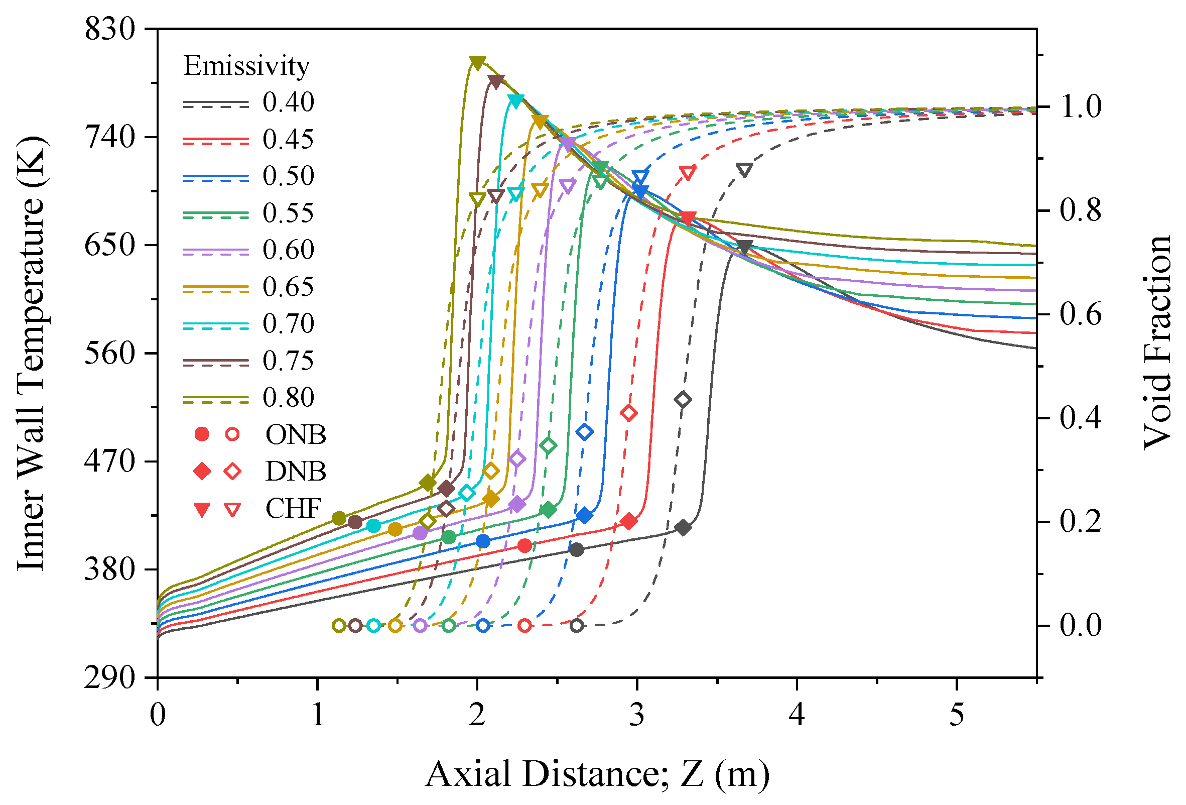
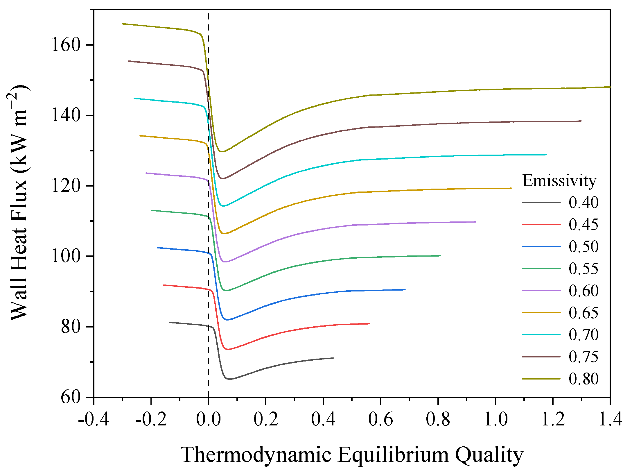
3.2. Wall Heat Flux and Inner Wall Temperature

Since the heat transferred into the inner pipe comes from the radiation outside it, and at the same time, the forced convective heat transfer between the pipe wall and the exterior flow has been taken into account. The distributions of wall heat flux and inner wall temperature are significantly different from the constant wall heat flux and constant wall temperature conditions. From the definition of the wall boundary conditions in the previous section, there is a strong correlation between the wall heat flux and inner wall temperature in the form of qw = aTw4 + bTw + c. Therefore, in this section, these two parameters are discussed together.
According to the criterion for the flow regime transition proposed by El Nakla et al. [12] and Mohanta et al. [19], flow film boiling can be divided into the IAFB regime at a void fraction of less than 0.5 and the DFFB regime at void fractions of greater than 0.9. The transition zone between these two regimes is regarded as the ISFB regime. However, since remarkable differences of the geometries and operating conditions exist in the reported investigations, the void fraction cannot be employed as an absolute criterion for flow regime transition. From these considerations, when the terms related to flow regimes are used in this article, they are only referring to approximate ranges, not the exact values.
Figure 15 and Figure 16 show the inner wall temperature distributions along the axial direction at inlet velocities of 0.3 m·s−1 to 1.0 m·s−1 and wall emissivity of 0.40 to 0.80, respectively. Void fraction is also shown in Figure 15 and Figure 16 for reflecting the two-phase flow state at the corresponding positions. Figure 17 and Figure 18 show the graphs of wall heat flux vs. thermodynamic equilibrium quality at different inlet velocity and pipe wall emissivity, respectively.
In Figure 15 and Figure 16, the DNB point is the location where the vapor phase temperature begins to exceed the saturation temperature, and the CHF point corresponds to the maximum wall temperature. It can be seen from Figure 15 and Figure 16 that in the single liquid convection region before the ONB point, the wall temperature increases linearly along the axial direction. Additionally, this trend of linear increase has continued into the negative thermodynamic equilibrium quality (xeq < 0) region when boiling occurs. In these regions, the increasing liquid temperature along the axial direction is the main reason for the increasing wall temperature. In the single-liquid-phase convection region, the liquid heats up due to convective heat transfer. In the negative thermodynamic equilibrium quality region where the DNB has not occurred, the vapor phase is at the saturation temperature, but the liquid phase is still in a subcooled state and approaching the saturation temperature gradually.
The pipe wall emissivity of each in Figure 15 case is 0.4. It can be seen from Figure 15 and Figure 17 that under this heating condition, inner wall temperature starts to increase dramatically, and the wall heat flux starts to decrease simultaneously when the thermodynamic equilibrium quality exceeds 0. During the process in which the value of thermodynamic equilibrium quality transits from negative to positive, the liquid core gradually heats up and approaches the saturation temperature. As a result, the bubble condensation rate decreases, which increases vapor film thickness and a deteriorated heat transfer coefficient. When xeq = 0, the void faction takes a value of 0.45 to 0.53, the DNB has already occurred, and the nucleate flow boiling regime has developed into the IAFB regime. As the void fraction increases along the pipe, the heat transfer continues to deteriorate and results in the occurrence of the CHF, where the heat transfer coefficient decreases to the minimum. At this time, the inner wall temperature is the highest, whereas the wall heat flux is the lowest, and the void fraction is about 0.88 to 0.9.
It can also be seen from Figure 15 and Figure 17 that in the post-CHF regime, the inner wall temperature decreases along the axial direction; meanwhile, the wall heat flux increases. This phenomenon has the same tendency as the IAFB at low pressure and low flow rate described in the experimental study of El Nakla et al. [12]. According to the conclusion drawn by El Nakla et al. [15], in the IAFB region before the CHF point, conduction is the dominant heat transfer mode of the vapor film, as the vapor film thickness increases along the pipe, the heat transfer coefficient falls off. However, in the region after the CHF point, where the IAFB gradually evolves into the IASB, the superheat temperature of the vapor phase increases. As a result, the evaporation rate is accelerated. At the same time, it leads to an increase in the velocity of the vapor phase, and convection becomes the primary heat transfer mode of the vapor phase. As the vapor phase velocity increases along the pipe, the convective heat transfer is improved, which finally results in an increase in wall heat flux and a decrease in inner wall temperature.
As the quality continues to increase, the void faction approaches to 1, the increase rate of wall heat flux and the decline rate of wall temperature are slowed down along the axial direction. This phenomenon is attributed to the IASB regime gradually evolving into the DFFB regime [12,15].
It can be seen from Figure 15 and Figure 17 that the maximum wall temperature corresponding to the CHF point decreases slightly with increasing inlet velocity. Meanwhile, the thermodynamic equilibrium quality at the CHF point decreases as the inlet velocity increases. When the inlet velocity is 0.3 m·s−1, the maximum wall temperature is 656.3 K, and when the inlet velocity is 0.8 m·s−1, the maximum wall temperature is 642.1 K. However, when the inlet flow velocity is 0.9 m·s−1, the DNB has occurred in the pipe, but the CHF has not reached. Furthermore, when the inlet velocity is 1.0 m·s−1, only the nucleate flow boiling is founded. The liquid temperature corresponding to the ONB point also decreases with the increase in inlet velocity. When the inlet velocity is 0.3 m·s−1, the wall temperature at the ONB point is 398.5 K. Additionally, when the inlet velocity is 1.0 m·s−1, the wall temperature of that point is 388.1 K. Since the boiling region is longer at a lower mass flow rate and the pressure drop of the boiling region is much larger than that of the single-phase convection area, lower inlet velocity results in higher static pressure at the ONB point which means a higher saturation temperature.
When the flow rate is constant, an increase in pipe wall emissivity enhances the radiative heat transfer intensity between the inner pipe and the outer pipe. It is another critical factor that affects the wall temperature and wall heat flux distributions. The higher wall emissivity causes higher inner wall temperature and wall heat flux in each regime, which are shown in Figure 16 and Figure 18.
It can be seen from Figure 16 that larger pipe wall emissivity results in a more obvious rise of wall temperature along the axial direction in the single-phase convection region, and a shorter distance between the inlet and the ONB point. The wall temperature at the ONB point rises as the wall emissivity increases, attributed to the higher static pressure and the higher saturation temperature at the ONB point caused by the boiling zone lengthening. It can also be seen from Figure 18 that under the higher wall emissivity condition, the thermodynamic equilibrium quality is lower at the ONB point, which means a lager average subcooled temperature of the liquid phase in that location. Under the condition that the inlet velocity is 0.5 m·s−1, when the wall emissivity is 0.4, the wall temperature of the ONB point is 396.4 K; and when the wall emissivity is 0.8, the wall temperature of that is 422.7 K. The maximum wall temperature at the CHF point is 649.7 K and 802.9 K when the wall emissivity is 0.4 and 0.8, respectively.
It can also be seen from Figure 16 and Figure 18 that, when the wall emissivity is low, the section where wall temperature starts to rise dramatically in the axial direction due to the DNB occurrence is in the positive thermodynamic equilibrium quality region. However, as the wall emissivity increases, the section where wall temperature rises dramatically approaches to a lower thermodynamic equilibrium quality region or even the negative thermodynamic equilibrium quality region. The CHF point also appears in a lower thermodynamic equilibrium quality as the wall emissivity increases. The higher wall emissivity leads to a more significant difference between the highest wall heat flux and the lowest wall heat flux, which appears at the ONB point and the CHF point, respectively.

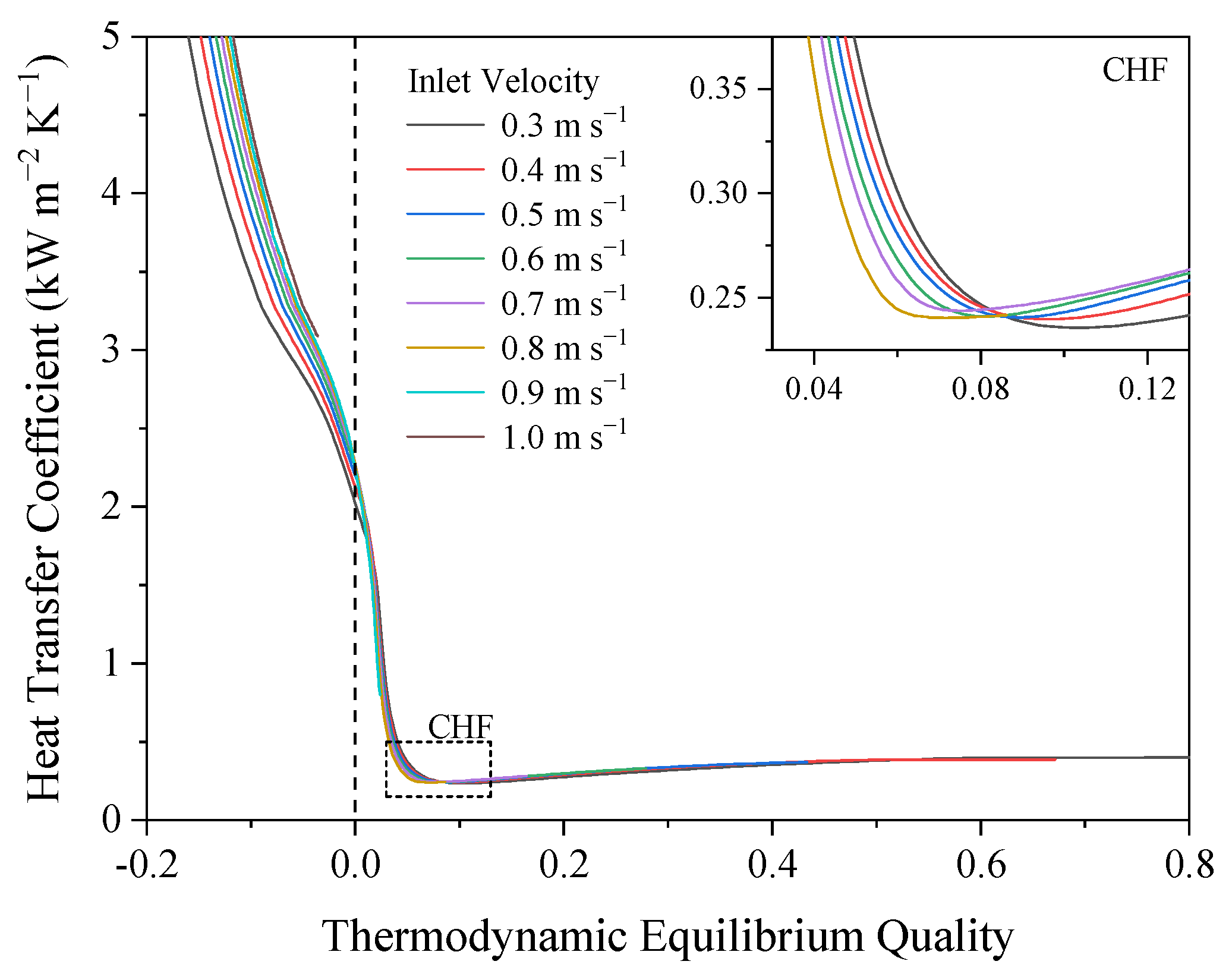
3.3. Heat Transfer Coefficient

Heat transfer coefficients are evaluated based on the difference between the inner wall temperature and the local saturation temperature. Figure 19 shows the heat transfer coefficient vs. thermodynamic equilibrium quality at the inlet velocity ranging from 0.3 m·s−1 to 1.0 m·s−1 under the wall emissivity of 0.4. Figure 20 shows the heat transfer coefficient data at the wall emissivity of 0.4 to 0.8 when the inlet velocity is 0.5 m·s−1. It can be seen from Figure 19 and Figure 20 that the heat transfer coefficient decreases rapidly before the CHF point, and increases slightly in the post-CHF region. There are two reasons for the decrease in heat transfer coefficient. One is that the subcooled temperature of the liquid core decreases gradually before the liquid phase reaches the saturation temperature as the boiling evolving, which results in the decrease in quenching heat flux term. Additionally, the other reason is the heat transfer deterioration caused by the occurrence of DNB.
As shown in Figure 19, in the negative equilibrium quality region, the heat transfer coefficient increases as the flow rate increases. However, in the positive equilibrium quality region, the variations of heat transfer coefficient with the equilibrium quality increasing at different flow rates are more uniform.
In Figure 20, the higher wall emissivity results in a lower heat transfer coefficient before the CHF point when the thermodynamic equilibrium quality is equal. In the nucleate flow boiling region, the value of quality mainly depends on the liquid phase temperature, since the mass fraction of the liquid phase is much larger than that of the vapor phase. When the equilibrium quality is equal, the liquid phase’s subcooled degree is almost equal, but the higher wall emissivity results in a more significant temperature gradient of the liquid phase along the radial direction. That is, the liquid phase has a higher temperature near the wall and a lower temperature in the center when the pipe has a higher emissivity. As a result, the wall temperature increases, and the heat transfer coefficient reduces as the wall emissivity increases. Similarly, when the DNB occurs on the wall, as the wall emissivity increases, temperature gradient of the liquid phase at this location is more significant, the subcooled degree of the liquid core is also larger. This explains why the DNB point approaches the negative equilibrium quality region as the wall emissivity increases. It can also be seen from Figure 20 that the heat transfer coefficient increases as the wall emissivity increases in the post-CHF region.

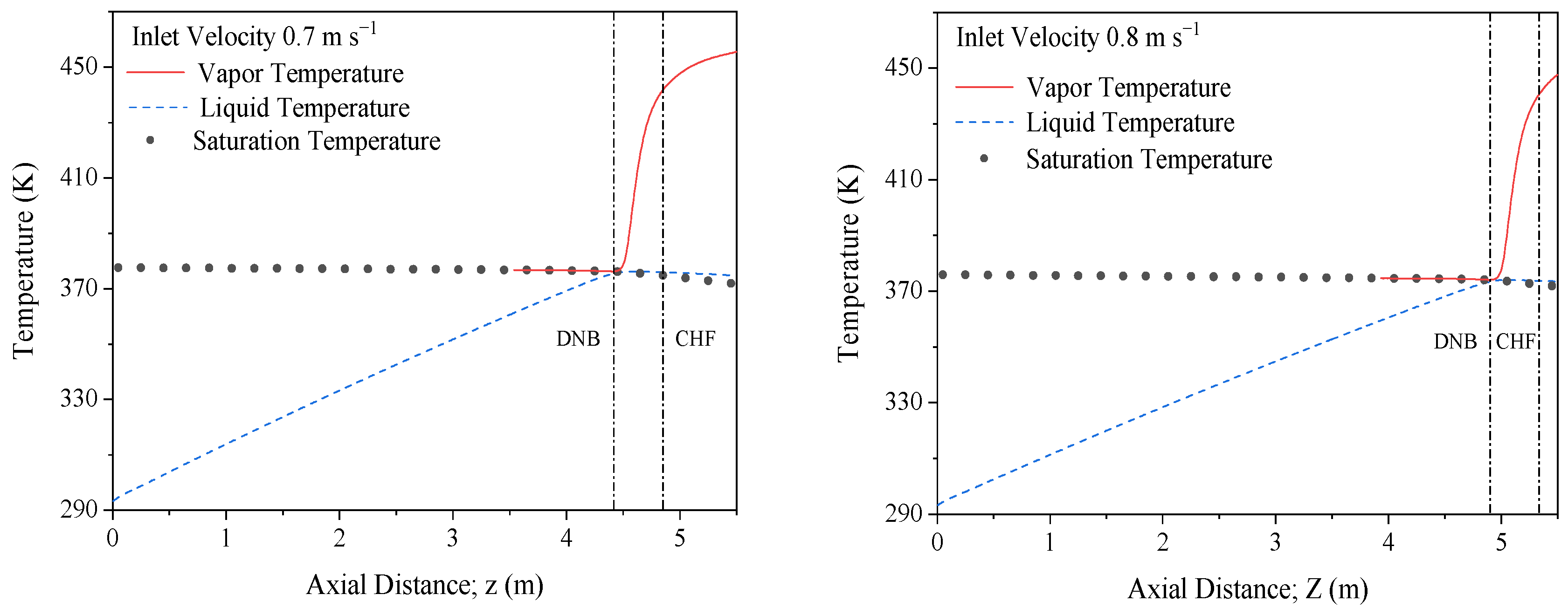
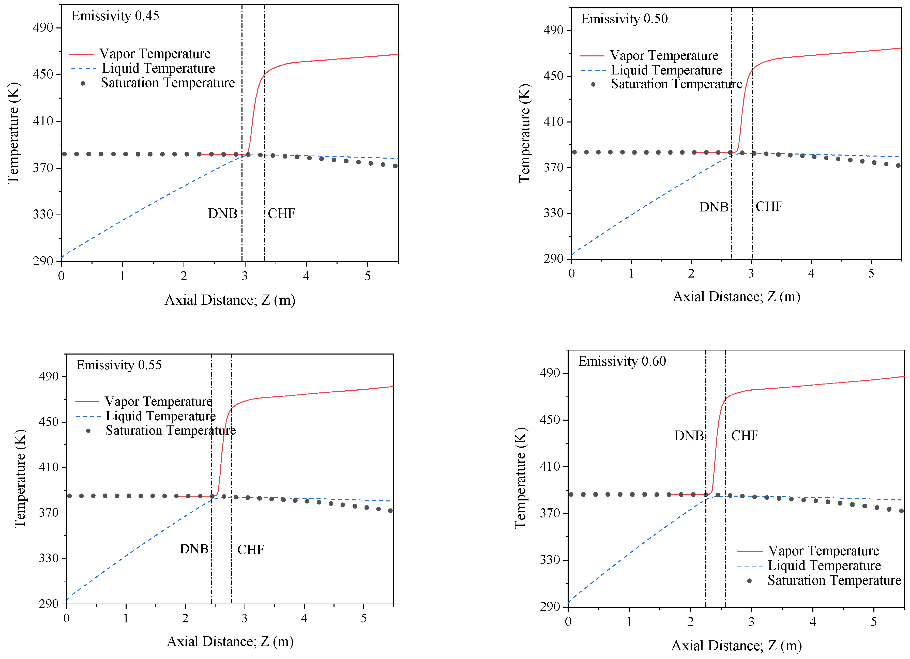
3.4. Temperature of Each Phase

Figure 21 and Figure 22 are the distributions of the average vapor temperature, the average liquid temperature and the local saturation temperature along the axial direction at the inlet velocities ranging from 0.3 m·s−1 to 0.8 m·s−1, and the wall emissivity ranging from 0.40 to 0.80, respectively.
Since the pressure drop in the single-phase convection region is much smaller than that in the boiling region, the saturation temperature gradually decreases along the axial direction in the boiling region. However, it is almost unchanged in the single-phase convention region. It can be seen from Figure 21 and Figure 22 that the vapor phase temperature is kept at the saturation temperature in the nucleate boiling region. When the DNB occurs, the superheated wall starts to heat the vapor phase directly, and the vapor temperature rises dramatically as a consequence. This dramatic rise in the vapor temperature continues until the CHF appears. In the post-CHF region, the increase in the vapor temperature decreases gradually and tends to stay in a fixed value, which results in a moderately linear increase in vapor temperature in the DFFB regime.
As shown in Figure 21 and Figure 22, the liquid temperature rises linearly along the axial direction in the single-phase convection region, and this trend continues into the nucleate boiling region. However, in the post-CHF region, the liquid phase temperature decreases along the axial direction due to the decreasing saturation temperature. Since the decrease rate of liquid phase temperature along the axial direction is lower than that of the local saturation temperature, the liquid temperature begins to exceed the saturation temperature. In other words, the liquid phase starts to be in a superheated state. Moreover, the superheated temperature of the liquid phase gradually increases along the axial direction in the post-CHF region. It can be reasonably referred that, as the velocity increases along the axial direction, the two-phase flow in the upstream is quickly transferred into the downstream, and the saturation temperature drops rapidly along the path. However, the liquid phase needs to reduce its temperature to the saturation temperature by evaporation, but the period during which the two-phase flow is transferred from the upstream to the downstream is not enough to complete the evaporation process. As a result, the superheated liquid phase appears in the pipe. The two-phase flow is in a non-equilibrium state, and the non-equilibrium effects are discussed in the next section.
In Figure 21, when the inlet velocity is 0.3 m·s−1, the vapor temperature at the outlet is the highest among other inlet velocity conditions with a value of 461.2 K, and the liquid phase temperature is 378.8 K with a superheat temperature of 7.2 K. In Figure 22, when the wall emissivity is 0.8, the vapor temperature at the outlet is the highest among other wall emissivity conditions with a value of 507.6 K, and the liquid phase temperature is 385.2 K with a superheat temperature of 13.6 K.
As the inlet velocity increases or wall emissivity decreases, the vapor phase temperature, liquid phase temperature, and the liquid phase superheat temperature all decrease at the outlet. In connection with the previous discussion, under the operating conditions employed in this work, neither the inner wall temperature nor the vapor temperature can reach the hydrocarbons’ pyrolysis temperature. However, it is sufficient to cause the phase change of the liquid hydrocarbons.

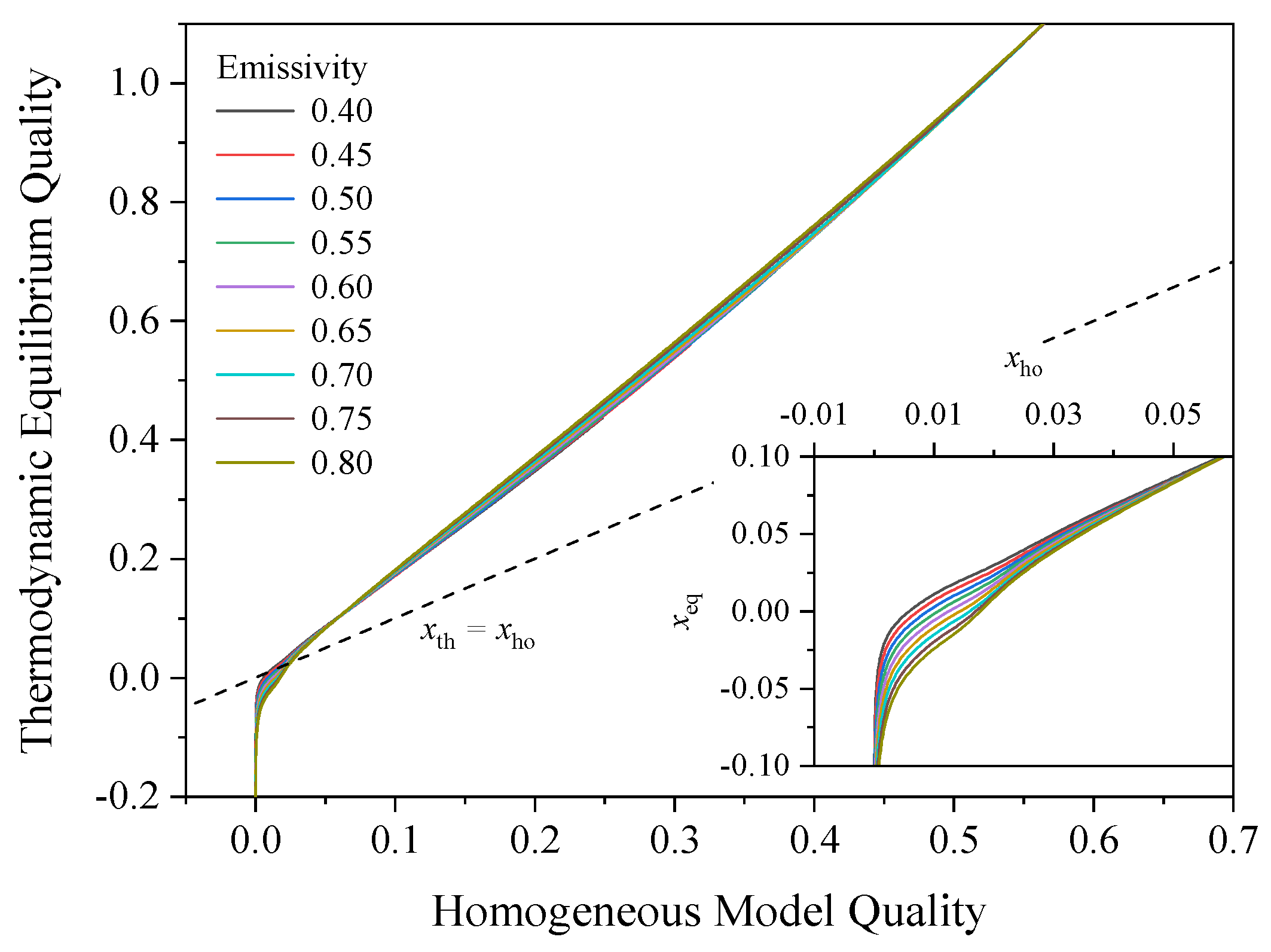
3.5. Non-Equilibrium Effect

The non-equilibrium effect prevails in both the subcooled boiling region and the post-CHF region [49,53]. The homogenous model quality is the mass fraction of the vapor phase, which is regarded as the actual vapor quality, whereas the thermodynamic equilibrium quality is a dimensionless parameter describing the specific enthalpy difference between the two-phase mixture and the saturated liquid. The difference between xho and xeq represents the specific enthalpy difference of the two-phase mixture in the non-equilibrium state and the equilibrium state, which can be used to characterize the non-equilibrium effect.
Figure 23 and Figure 24 are the graphs of homogenous model quality vs. thermodynamic equilibrium quality at the inlet velocity of 0.3 m·s−1 to 0.8 m·s−1 and wall emissivity of 0.40 to 0.80, respectively. The non-equilibrium effect prevails in both of the negative equilibrium quality regions and the positive equilibrium quality region. As shown in Figure 23 and Figure 24, the negative equilibrium quality region is below the xeq = xho line, and the non-equilibrium effect is mainly caused by liquid phase subcooling. Most of the positive equilibrium quality region is above the xeq = xho line, and the non-equilibrium effect increases with the increasing homogeneous model quality. The non-equilibrium phenomenon in this region is caused by the increase in vapor phase temperature and the decrease in saturation temperature. It can be concluded from Figure 23 that in the post-CHF region, the non-equilibrium effect is more evident at a larger the inlet velocity when the homogeneous model quality is equal. However, in Figure 24, the non-equilibrium effect is slightly affected by the variations in wall emissivity.

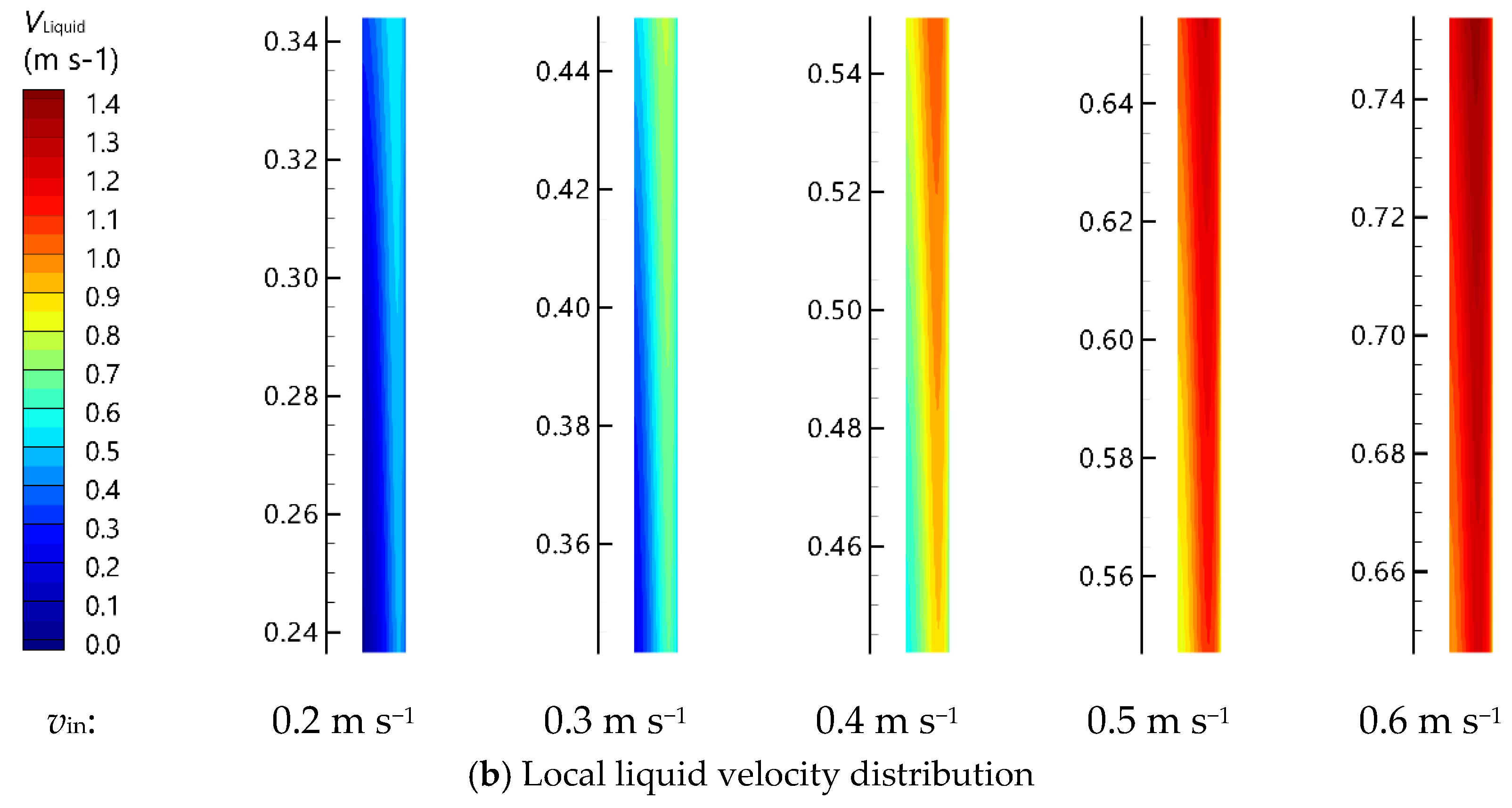
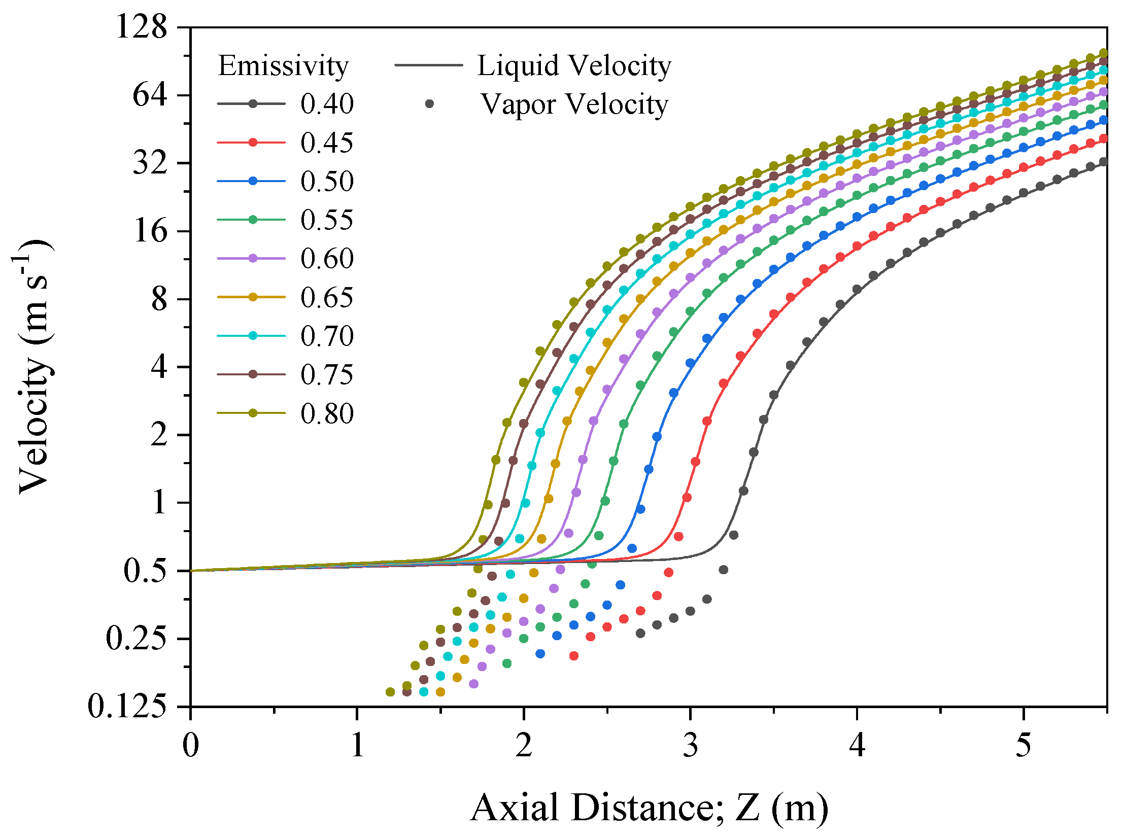
3.6. Velocity of Each Phase
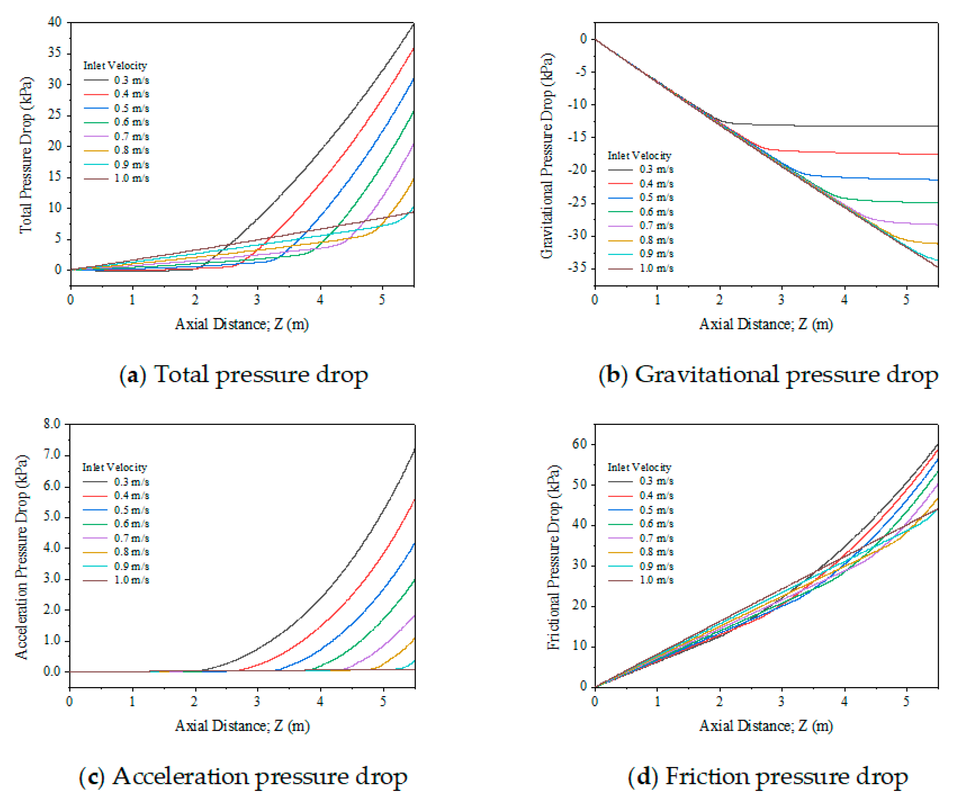
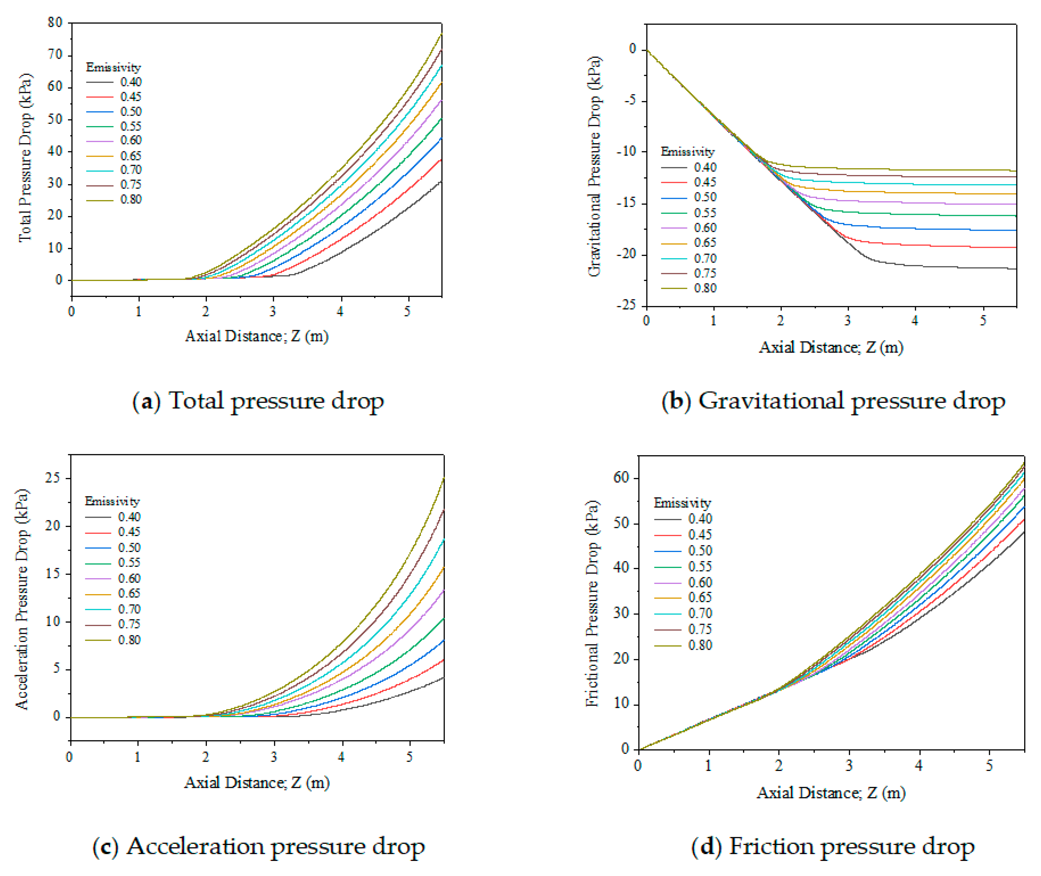
Figure 25 and Figure 26 shows the distribution of average vapor phase velocity and average liquid phase velocity along the axial direction at the inlet velocity of 0.3 m·s−1 to 0.8 m·s−1 and the wall emissivity of 0.40 to 0.80, respectively. As shown in Figure 25 and Figure 26, in the single-phase convection region, the liquid velocity increases slowly along the axial direction due to the decreases in density caused by temperature rise. At the beginning of boiling, bubbles start to be generated on the wall, the void fraction is extremely low, and the liquid phase velocity does not increase significantly immediately. Meanwhile, the vapor phase velocity is significantly less than the liquid phase’s average velocity, since the bubbles are generated on the wall where the liquid phase velocity is much slower than in the center of the pipe.
As the boiling evolves, both the liquid phase velocity and vapor phase velocity increase along the axial direction. Moreover, as the bubbles depart from the wall and move towards the center of the pipe due to the lift force, the difference between the velocity of the vapor phase and the liquid phase is gradually eliminated. In the post-CHF region, as the quality increases linearly along the axial direction, the vapor phase velocity continues to rise and eventually exceeds the liquid phase velocity. Additionally, the premier phase converts from the liquid phase to the vapor phase. It can be seen from Figure 25 that the smaller inlet velocity leads to a higher velocity of each phase at the outlet. Additionally, the outlet velocity of each phase increases with the wall emissivity increasing as shown Figure 26.

3.7. Pressure Drop

The pressure drop of two-phase in the lance is an essential parameter for the process control and optimization. Predicting the pressure drop components is of great significance to ensure the safe operation of the furnace.
Figure 27 shows the distributions of the total pressure drop and its components along the axial direction at different inlet velocities. The total pressure drop is shown in Figure 27a, the variation rate of the single-phase convection region and nucleate boiling region is much lower than the regions downstream of the DNB point. As the inlet velocity increases, the variation rate increases in both the single-phase convection region and the two-phase flow region. Since the larger inlet velocity results in a shorter boiling region within the pipe, the total pressure drop of the entire pipe decreases as the inlet velocity increases.
Figure 27b is the graph of the gravitational term. Since the fluid flows vertically downward, the gravitational pressure drop has a negative value, which means the gravitational potential energy is converted into kinetic energy. In Figure 27b, a linear decrease in the gravitational pressure drop is observed in the region before the DNB point. Additionally, in the region downstream of the DNB, the variation rate gradually falls off.
Figure 27c shows the distribution of acceleration term. The acceleration pressure drop in the single-phase convection region is caused by the density variation, and it is too small to take into account. The significant variation of the acceleration pressure drop is observed in the boiling region after the occurrence of DNB. The acceleration pressure drop is relatively smaller compared with the total pressure drop. The higher inlet velocity leads to a lager acceleration pressure drop of the entire pipe.
The frictional pressure drop is shown in Figure 27d, which is derived from the total pressure drop, gravitational pressure drop, and acceleration pressure drop. The variation rate of frictional pressure drop along the axial direction increases with the flow rate increasing either in the single-phase convection region or in the two-phase flow region. Moreover, the variation rate of frictional pressure drop rises as boiling evolves. In the single-phase convection region, as well as the region before the DNB, the fractional pressure drop is offset by the gravitational pressure drop to some extent, and the total pressure drop turns out to vary moderately along the axial direction. However, in the region downstream of the DNB, the effect of gravitational pressure drop is gradually eliminated, and the total pressure drop begins to rise significantly.
Figure 28 shows the pressure drop distributions along the axial direction at wall emissivity ranging from 0.4 to 0.8. Figure 28a is the total pressure drop, Figure 28b–d are the gravitational term, acceleration term and the fractional term, respectively. The total pressure drop of the entire pipe rises as the wall emissivity increases. The gravitational pressure drop in Figure 28b shows the same trend as Figure 27b, its value is mainly determined by the length of the pipe before the DNB. The higher wall emissivity results in a more significant acceleration pressure drop of the entire pipe, as well as a higher increase rate of that along the axial direction. Additionally, the frictional pressure drop also increases as the wall emissivity increases.

4. Conclusions

In this study, a numerical model was developed by employing the improved RPI model for the flow boiling of subcooled n-heptane within the TSL lance. The vertical downward flow is heated by the external radiation and external convective heat transfer. The heat transfer and flow characteristics of n-heptane from the single-phase convection regime to the DFFB regime under different mass flow rates and wall emissivity conditions were investigated. The main conclusions are as follows:
(1)
As the inlet velocity decreases or the wall emissivity increases, the ONB location approaches the inlet and the void fraction near the outlet increases. The path through which the single-liquid-phase flow converts into the DFFB with a void fraction higher than 0.9 is shorter. Moreover, the increase rate of void fraction gradually decreases along the axial direction after the void fraction reaches 0.9.
(2)
The maximum wall temperature corresponding to the CHF point decreases slightly with the increase in inlet velocity but increases significantly with the increase in wall emissivity.
(3)
The variations in flow rate barely influence the value of thermodynamic equilibrium quality at the location of the DNB and the CHF. However, increasing the wall emissivity results in a smaller thermodynamic equilibrium quality at the DNB point and the CHF point.
(4)
The heat transfer coefficient is greatly affected by the flow rate in the negative thermodynamic equilibrium quality region; the heat transfer coefficient increases as the flow rate increases at the same equilibrium quality condition. In the positive equilibrium quality region, the heat transfer coefficient varies more uniformly with the equilibrium quality at different flow rates. Under the same equilibrium quality condition, the heat transfer coefficient decreases in the negative equilibrium quality region and increases in the post-CHF region with the wall emissivity increasing.
(5)
As the flow rate decreases or wall emissivity increases, the average temperature and the average velocity of each phase at the outlet increases.
(6)
The non-equilibrium effect is evident in the subcooled boiling region and the post-CHF region. The non-equilibrium effect in the subcooled boiling region contributes to the subcooled liquid phase. Additionally, in the post-CHF region, the non-equilibrium effect is caused by the superheated vapor phase and the superheated liquid phase. The flow rate increasing and wall emissivity reducing both lead to a more significant non-equilibrium effect at the outlet.
(7)
Since the frictional pressure drop is offset by the gravitational pressure drop in the regions before the DNB to some extent, the total pressure drop varies moderately along the axial direction. However, as the gravitational pressure drop falls off gradually in the post-CHF region, and the total pressure drop varies more obviously. Higher wall emissivity results in a larger total pressure drop of the entire pipe. However, for different flow rate conditions, the total pressure drop of the entire pipe is affected by both the flow rate and the length of the boiling region.

Author Contributions

Conceptualization, X.H.; methodology, X.H.; software, J.L. and L.C.; validation, J.L. and L.C.; data curation, J.L.; writing—original draft preparation, J.L.; writing—review and editing, X.Z., X.H. and L.C.; visualization, L.C.; supervision, X.Z.; project administration, X.Z.; funding acquisition, X.Z. All authors have read and agreed to the published version of the manuscript.

Funding

This research was funded by the Natural Science Foundation of China (51966005) and the Yunnan Fundamental Research Projects (202101AT070120).

Data Availability Statement

All data are included in the manuscript.

Acknowledgments

This work was supported by the Yunnan Fundamental Research Projects (No. 202101AT070120) and the Natural Science Foundation of China (No. 51966005). We also thank Shiming Zhang and Shan Qing for their help in this research.

Conflicts of Interest

The authors declare no conflict of interest.

Nomenclature

AArea, (m2)
CpLSpecific heat of liquid phase, (J/kg K)
DWDeparture diameter of bubbles, (m)
fBubble departure frequency
FForce, (N)
FD,iDrag force, (N)
FL,iLift force, (N)
FW,iWall lubrication force, (N)
FTD,iTurbulent dispersion force, (N)
FVM,iVirtual mass force, (N)
GMass flux, (kg/m2 s)
I = Unit tensor
JasubSubcooled Jacob number
klThermal conductivity of the liquid phase, (W/m k)
KEmpirical constant
m ˙ ji Mass transfer coefficient from the i to j phase
pStatic pressure, (Pa)
ptotTotal pressure drop, (Pa)
qHeat flux
qwWall heat flux, (W/m2)
qCConvective heat flux, (W/m2)
qEEvaporative heat flux, (W/m2)
qraRadiant heat transfer, (W/m2)
SMMass source term, (K)
SEEnergy source term, (K)
TOTemperature of the outer pipe wall, (K)
TITemperature of the inner pipe wall, (K)
TairAir temperature, (K)
TWWall temperature, (K)
TLLiquid temperature, (K)
TsatSaturation temperature, (K)
vVelocity, (m/s)
Greek
εOEmissivity of the outer pipe wall
εIEmissivity of the inner pipe wall
σStefan-Boltzmann constant
αVolume fraction
ρdensity
Subscripts
OOuter pipe
IInner pipe
bBubbles
WWall
VVapor
LLiquid
CConvective heat flux
EEvaporative heat flux
MMass
satSaturation
iPhase i
jPhase j
Abbreviations
TSLTop Submerged Lance
CHFCritical Heat Flux
DFFBDispersed Flow Film Boiling
RPIRensselaer Polytechnic Institute
DNBDeparture from Nucleate Boiling
IAFBInverted Annular Film Boiling
ISFBInverted Slug Film Boiling

References

  1. Schlesinger, M.E.; King, M.J.; Davenport, W.G. Extractive Metallurgy of Copper; Elsevier: Amsterdam, The Netherlands, 2011. [Google Scholar]
  2. Deng, W.; Zhang, X.; Wang, H.; Feng, L.; Zhang, H.; Zhang, G. Dispersion characteristics of biodiesel spray droplets in top-blown injection smelting process. Chem. Eng. Process. Process Intensif. 2018, 126, 168–177. [Google Scholar] [CrossRef]
  3. Alvear, R.G.; Hunt, P.S.; Zhang, B. Copper ISASMELT—Dealing with Impurities. In Advanced Processing of the Metals and Materials, Sohn International Symposium, San Diego, CA, USA, 27–31 August 2006; Kongoli, F., Reddy, R.G., Eds.; Wiley: Hoboken, NJ, USA, 2006; pp. 673–685. [Google Scholar]
  4. Krepper, E.; Končar, B.; Egorov, Y. CFD modelling of subcooled boiling—Concept, validation and application to fuel assembly design. Nucl. Eng. Des. 2007, 237, 716–731. [Google Scholar] [CrossRef]
  5. Vadlamudi, S.R.G.; Nayak, A.K. CFD simulation of Departure from Nucleate Boiling in vertical tubes under high pressure and high flow conditions. Nucl. Eng. Des. 2019, 352, 110150. [Google Scholar] [CrossRef]
  6. Wojtan, L.; Ursenbacher, T.; Thome, R.J. Investigation of flow boiling in horizontal tubes: Part II—Development of a new heat transfer model for stratified-wavy, dryout and mist flow regimes. Int. J. Heat Mass Transf. 2005, 48, 2970–2985. [Google Scholar] [CrossRef]
  7. Arcanjo, A.A.; Tibiriçá, C.B.; Ribatski, G. Evaluation of flow patterns and elongated bubble characteristics during the flow boiling of halocarbon refrigerants in a micro-scale channel. Exp. Therm. Fluid Sci. 2010, 34, 766–775. [Google Scholar] [CrossRef]
  8. Hu, G.; Ma, Y.; Liu, Q. Evaluation on Coupling of Wall Boiling and Population Balance Models for Vertical Gas-Liquid Subcooled Boiling Flow of First Loop of Nuclear Power Plant. Energies 2021, 14, 7357. [Google Scholar] [CrossRef]
  9. Saisorn, S.; Wongpromma, P.; Wongwises, S. The difference in flow pattern, heat transfer and pressure drop char-acteristics of mini-channel flow boiling in horizontal and vertical orientations. Int. J. Multiph. Flow 2018, 101, 97–112. [Google Scholar] [CrossRef]
  10. Bediako, E.G.; Dančová, P.; Vít, T. Experimental study of horizontal flow boiling heat transfer coefficient and pressure drop of R134afrom subcooled liquid region to superheated vapor region. Energies 2022, 15, 681. [Google Scholar] [CrossRef]
  11. Wang, J.; Zhu, S.; Xie, J. Investigation of R290 Flow Boiling Heat Transfer and Exergy Loss in a Double-Concentric Pipe Based on CFD. Energies 2021, 14, 7121. [Google Scholar] [CrossRef]
  12. El Nakla, M.; Groeneveld, D.; Cheng, S. Experimental study of inverted annular film boiling in a vertical tube cooled by R-134a. Int. J. Multiph. Flow 2011, 37, 67–75. [Google Scholar] [CrossRef]
  13. Shah, M.M. A General Predictive Technique for Heat Transfer during Saturated Film Boiling in Tubes. Heat Transf. Eng. 1980, 2, 51–62. [Google Scholar] [CrossRef]
  14. Shah, M.M.; Siddiqui, M.A. A general correlation for heat transfer during dispersed-flow film boiling in tubes. Heat Transf. Eng. 2000, 21, 18–32. [Google Scholar]
  15. Shah, M.M. Comprehensive correlation for dispersed flow film boiling heat transfer in mini/macro tubes. Int. J. Refrig. 2017, 78, 32–46. [Google Scholar] [CrossRef]
  16. Liu, Q.; Sun, X. Wall heat transfer in the inverted annular film boiling regime. Nucl. Eng. Des. 2020, 363, 110660. [Google Scholar] [CrossRef]
  17. Hammouda, N.; Groeneveld, D.; Cheng, S. An experimental study of subcooled film boiling of refrigerants in vertical up-flow. Int. J. Heat Mass Transf. 1996, 39, 3799–3812. [Google Scholar] [CrossRef]
  18. Hammouda, N.; Groeneveld, D.; Cheng, S. Two-fluid modelling of inverted annular film boiling. Int. J. Heat Mass Transf. 1997, 40, 2655–2670. [Google Scholar] [CrossRef]
  19. Mohanta, L.; Riley, M.P.; Cheung, F.B.; Bajorek, S.M.; Kelly, J.M.; Tien, K.; Hoxie, C.L. Experimental Investigation of Inverted Annular Film Boiling in a Rod Bundle during Reflood Transient. Nucl. Technol. 2015, 190, 301–312. [Google Scholar] [CrossRef]
  20. Mohanta, L.; Sohag, F.A.; Cheung, F.-B.; Bajorek, S.M.; Kelly, J.M.; Tien, K.; Hoxie, C.L. Heat transfer correlation for film boiling in vertical upward flow. Int. J. Heat Mass Transf. 2017, 107, 112–122. [Google Scholar] [CrossRef]
  21. Xu, Y.; Fang, X. A new correlation of two-phase frictional pressure drop for evaporating flow in pipes. Int. J. Refrig. 2012, 35, 2039–2050. [Google Scholar] [CrossRef]
  22. Müller-Steinhagen, H.; Heck, K. A simple friction pressure drop correlation for two-phase flow in pipes. Chem. Eng. Process. Process Intensif. 1986, 20, 297–308. [Google Scholar] [CrossRef]
  23. Xu, Y.; Fang, X.; Li, D.; Li, G.; Yuan, Y.; Xu, A. An experimental study of flow boiling frictional pressure drop of R134a and evaluation of existing correlations. Int. J. Heat Mass Transf. 2016, 98, 150–163. [Google Scholar] [CrossRef]
  24. Muszynski, T.; Andrzejczyk, R.; Dorao, C.A. Detailed experimental investigations on frictional pressure drop of R134a during flow boiling in 5 mm diameter channel: The influence of acceleration pressure drop component. Int. J. Refrig. 2017, 82, 163–173. [Google Scholar] [CrossRef]
  25. Zivi, S.M. Estimation of steady-state steam void-fraction by means of the principle of minimum entropy production. J. Heat Transder 1964, 86, 247–251. [Google Scholar] [CrossRef]
  26. Vadlamudi, S.R.G.; Nayak, A.K. Review of literature on departure from nucleate boiling in subcooled flow boiling. Multiph. Sci. Technol. 2018, 30, 247–266. [Google Scholar] [CrossRef]
  27. Murallidharan, J.S.; Prasad BV SS, S.; Patnaik BS, V.; Hewitt, G.F.; Badalassi, V. CFD investigation and as-sessment of wall heat flux partitioning model for the prediction of high pressure subcooled flow boiling. Int. J. Heat Mass Transf. 2016, 103, 211–230. [Google Scholar] [CrossRef]
  28. Colombo, M.; Fairweather, M. Accuracy of Eulerian–Eulerian, two-fluid CFD boiling models of subcooled boiling flows. Int. J. Heat Mass Transf. 2016, 103, 28–44. [Google Scholar] [CrossRef]
  29. Kurul, N. On the modeling of multidimensional effects in boiling channels. In Proceedings of the ANS. Proc. National Heat Transfer Conference, Minneapolis, MN, USA, 28–31 July 1991. [Google Scholar]
  30. Tu, J.; Yeoh, G. On numerical modelling of low-pressure subcooled boiling flows. Int. J. Heat Mass Transf. 2002, 45, 1197–1209. [Google Scholar] [CrossRef]
  31. Zhang, R.; Cong, T.; Tian, W.; Qiu, S.; Su, G. Effects of turbulence models on forced convection subcooled boiling in vertical pipe. Ann. Nucl. Energy 2015, 80, 293–302. [Google Scholar] [CrossRef]
  32. Talebi, S.; Abbasi, F.; Davilu, H. A 2D numerical simulation of sub-cooled flow boiling at low-pressure and low-flow rates. Nucl. Eng. Des. 2009, 239, 140–146. [Google Scholar] [CrossRef]
  33. Tao, H.-Z.; Xie, C.-Y.; Wang, M.-M. Numerical simulation study on the flow and heat transfer characteristics of sub-cooled boiling in vertical round and flattened tubes. Ann. Nucl. Energy 2019, 140, 107144. [Google Scholar] [CrossRef]
  34. Gu, J.; Wang, Q.; Wu, Y.; Lyu, J.; Li, S.; Yao, W. Modeling of subcooled boiling by extending the RPI wall boiling model to ultra-high pressure conditions. Appl. Therm. Eng. 2017, 124, 571–584. [Google Scholar] [CrossRef]
  35. Pothukuchi, H.; Kelm, S.; Patnaik, B.; Prasad, B.; Allelein, H.-J. CFD modeling of critical heat flux in flow boiling: Validation and assessment of closure models. Appl. Therm. Eng. 2019, 150, 651–665. [Google Scholar] [CrossRef]
  36. Lavieville, J.; Quemerais, E.; Mimouni, S.; Boucker, M.; Mechitoua, N. NEPTUNE CFD V1. 0 theory manual. Rapport Interne EDF H-I81-2006-04377-EN. Rapport NEPTUNE Nept_2004_L 2006, 1, 3. [Google Scholar]
  37. Zhang, R.; Cong, T.; Tian, W.; Qiu, S.; Su, G. Prediction of CHF in vertical heated tubes based on CFD methodology. Prog. Nucl. Energy 2015, 78, 196–200. [Google Scholar] [CrossRef]
  38. Celata, G.; Cumo, M.; Mariani, A. Burnout in highly subcooled water flow boiling in small diameter tubes. Int. J. Heat Mass Transf. 1993, 36, 1269–1285. [Google Scholar] [CrossRef]
  39. Li, Q.; Avramova, M.; Jiao, Y.; Chen, P.; Yu, J.; Pu, Z.; Chen, J. CFD prediction of critical heat flux in vertical heated tubes with uniform and non-uniform heat flux. Nucl. Eng. Des. 2018, 326, 403–412. [Google Scholar] [CrossRef]
  40. Maytorena, V.; Hinojosa, J. Three-dimensional numerical study of direct steam generation in vertical tubes receiving concentrated solar radiation. Int. J. Heat Mass Transf. 2019, 137, 413–433. [Google Scholar] [CrossRef]
  41. Končar, B.; Borut, M. Wall function approach for boiling two-phase flows. Nucl. Eng. Des. 2010, 240, 3910–3918. [Google Scholar] [CrossRef]
  42. Mali, C.R.; Vinod, V.; Patwardhan, A.W. Comparison of phase interaction models for high pressure subcooled boiling flow in long vertical tubes. Nucl. Eng. Des. 2017, 324, 337–359. [Google Scholar] [CrossRef]
  43. Chen, J.; Zeng, R.; Zhang, X.; Qiu, L.; Xie, J. Numerical modeling of flow film boiling in cryogenic chilldown process using the AIAD framework. Int. J. Heat Mass Transf. 2018, 124, 269–278. [Google Scholar] [CrossRef]
  44. Lillo, G.; Mastrullo, R.; Mauro, A.; Viscito, L. Flow boiling heat transfer, dry-out vapor quality and pressure drop of propane (R290): Experiments and assessment of predictive methods. Int. J. Heat Mass Transf. 2018, 126, 1236–1252. [Google Scholar] [CrossRef]
  45. Daubert, T.E.; Danner, R.P. API Technical Data Book Petroleum Refining: American Petroleum Institute; API: Washington, DC, USA, 1997. [Google Scholar]
  46. Beaton, C.F.; Hewitt, G.F. (Eds.) Physical Property Data for the Design Engineer; Hemisphere: New York, NY, USA, 1989; p. 394. [Google Scholar]
  47. Zhao, H.; Lu, T.; Yin, P.; Mu, L.; Liu, F. An Experimental and Simulated Study on Gas-Liquid Flow and Mixing Behavior in an ISASMELT Furnace. Metals 2019, 9, 565. [Google Scholar] [CrossRef] [Green Version]
  48. Xu, Y.; Fang, X. Correlations of void fraction for two-phase refrigerant flow in pipes. Appl. Therm. Eng. 2014, 64, 242–251. [Google Scholar] [CrossRef]
  49. He, H.; Pan, L.-M.; Wei, L.; Zhang, M.-H.; Zhang, D.-F. On the importance of non-equilibrium effect in microchannel two-phase boiling flow. Int. J. Heat Mass Transf. 2019, 149, 119185. [Google Scholar] [CrossRef]
  50. Kuang, Y.; Wang, W.; Miao, J.; Zhang, H. Non-linear analysis of nitrogen pressure drop instability in mi-cro/mini-channels. Int. J. Heat Mass Transf. 2020, 147, 118953. [Google Scholar] [CrossRef]
  51. Huang, H.; Thome, J.R. An experimental study on flow boiling pressure drop in multi-microchannel evaporators with different refrigerants. Exp. Therm. Fluid Sci. 2017, 80, 391–407. [Google Scholar] [CrossRef]
  52. Chen, J.C. Correlation for Boiling Heat Transfer to Saturated Fluids in Convective Flow. Ind. Eng. Chem. Process Des. Dev. 1966, 5, 322–329. [Google Scholar] [CrossRef] [Green Version]
  53. Wang, Y.-J.; Pan, C. A one-dimensional semi-empirical model considering transition boiling effect for dispersed flow film boiling. Nucl. Eng. Des. 2017, 316, 99–111. [Google Scholar] [CrossRef]
Figure 1. Schematic diagram of the TSL lance.
Energies 15 03777 g001
Figure 2. (a) Schematic of computational domain and (b) local mesh structure.
Energies 15 03777 g002
Figure 3. Schematic diagram of the vertical pipe.
Energies 15 03777 g003
Figure 4. Local mesh structure.
Energies 15 03777 g004
Figure 5. Local void fraction and liquid phase velocity distribution near the position.
Energies 15 03777 g005aEnergies 15 03777 g005b
Figure 6. Heat transfer coefficient comparisons between simulated results and Chen’s correlation.
Energies 15 03777 g006
Figure 7. Void fraction distribution along the axial direction at inlet velocities from 0.3 m·s−1 to 1.0 m·s−1.
Energies 15 03777 g007
Figure 8. Void fraction distribution along the axial direction under wall emissivity from 0.40 to 0.80.
Energies 15 03777 g008
Figure 9. Homogeneous model quality distribution along the axial direction at inlet velocities from 0.3 m·s−1 to 1.0 m·s−1 (Dashed lines are void fraction).
Energies 15 03777 g009
Figure 10. Homogeneous model quality distribution along the axial direction under wall emissivity from 0.40 to 0.80 (Dashed lines are void fraction).
Energies 15 03777 g010
Figure 11. Local void fraction distributions at inlet velocities ranging from 0.3 m·s−1 to 1.0 m·s−1 (x-axis is the axial distance).
Energies 15 03777 g011aEnergies 15 03777 g011b
Figure 12. Local void fraction distributions under wall emissivity ranging from 0.40 to 0.80 (x-axis is the axial distance).
Energies 15 03777 g012aEnergies 15 03777 g012b
Figure 13. Homogeneous model quality distributions at inlet velocities ranging from 0.3 m·s−1 to 0.8 m·s−1.
Energies 15 03777 g013
Figure 14. Homogeneous model quality distributions under wall emissivity ranging from 0.40 to 0.80.
Energies 15 03777 g014
Figure 15. Inner wall temperature distributions along the axial direction at inlet velocities of 0.3 m·s−1 to 1.0 m·s−1.
Energies 15 03777 g015
Figure 16. Inner wall temperature distributions along the axial direction under wall emissivity from 0.40 to 0.80.
Energies 15 03777 g016
Figure 17. Wall heat flux vs. thermodynamic equilibrium quality at inlet velocities from 0.3 m·s−1 to 1.0 m·s−1.
Energies 15 03777 g017
Figure 18. Wall heat flux vs. thermodynamic equilibrium quality under wall emissivity from 0.40 to 0.80.
Energies 15 03777 g018
Figure 19. Heat transfer coefficient vs. thermodynamic equilibrium quality at inlet velocities of 0.3 m·s−1 to 1.0 m·s−1.
Energies 15 03777 g019
Figure 20. Heat transfer coefficient vs. thermodynamic equilibrium quality under wall emissivity of 0.40 to 0.80.
Energies 15 03777 g020
Figure 21. Distributions of average vapor temperature, average liquid temperature and local saturation temperature along the axial direction at inlet velocities ranging from 0.3 m·s−1 to 0.8 m·s−1.
Energies 15 03777 g021aEnergies 15 03777 g021b
Figure 22. Distributions of average vapor temperature, average liquid temperature and local saturation temperature along the axial direction under wall emissivity ranging from 0.40 to 0.80.
Energies 15 03777 g022aEnergies 15 03777 g022b
Figure 23. Homogenous model quality vs. thermodynamic equilibrium quality at inlet velocities of 0.3 m·s−1 to 0.8 m·s−1.
Energies 15 03777 g023
Figure 24. Homogenous model quality vs. thermodynamic equilibrium quality under wall emissivity of 0.40 to 0.80.
Energies 15 03777 g024
Figure 25. Average velocity of vapor phase and liquid phase along the axial direction at inlet velocities of 0.3 m·s−1 to 0.8 m·s−1.
Energies 15 03777 g025
Figure 26. Average velocity of vapor phase and liquid phase along the axial direction under wall emissivity of 0.40 to 0.80.
Energies 15 03777 g026
Figure 27. Distributions of the total pressure drop and its components along the axial direction at inlet velocities of 0.3 m·s−1 to 1.0 m·s−1.
Energies 15 03777 g027
Figure 28. Distributions of the total pressure drop and its components along the axial direction under wall emissivity of 0.40 to 0.80.
Energies 15 03777 g028
Table 1. Detailed parameters of a typical TSL furnace.
NameUnitValue
Furnace Heightm7.173
Furnace Diameterm3.84
Lance Diameterm0.303–0.4
Molten Bath Levelm1.85–2
Lance Submergence Depthm0.3
Table 2. Operating conditions for simulation.
Series 1Series 2
Inlet Velocity (m·s−1)0.3, 0.4, 0.5, 0.6,
0.7, 0.8, 0.9, 1.0
0.5
Inlet Temperature (K)293.15293.15
Inner Pipe Wall Emissivity0.400.40, 0.45, 0.50, 0.55, 0.60,
0.65, 0.70, 0.75, 0.80
Outer Pipe Temperature (K)14001400
Oxygen-enriched Air Temperature (K)293.15293.15
External Heat Transfer Coefficient (W·m−2·K−1)5050
Operating Pressure (atm)11
Table 3. Model Settings.
Model CategoryModel Selection
Turbulence ModelStandard k-ε Model
Wall Function: Non-equilibrium Wall Function
Turbulence Multiphase Model: Per Phase
Interphase Force ModelDrag Force Model: Universal Drag Model
Lift Force Model: Moraga Model
Wall Lubrication Force: No Wall Lubricating Force
Turbulence Dispersion Force: Lopez de Bertodano Model
Turbulence Interaction Force: Troshko-Hassan Model
Interfacial Heat Transfer ModelHughmark Model
Interfacial Area Concentration ModelSymmetric IAC Model
Correlation of Bubble DiameterUnal Correlation
Table 4. Operating conditions for model validation.
Series 1Series 2
Inlet Velocity (m s−1)0.2, 0.3, 0.4, 0.5, 0.60.6
Inlet Subcooling (K)0.50.5
Wall Heat Flux (kW m−2)1012, 14, 16, 18,
20, 22, 24, 26
Publisher’s Note: MDPI stays neutral with regard to jurisdictional claims in published maps and institutional affiliations.

